1. Introduction
The interaction between a deformable body and a moving fluid has received remarkable attention due to its numerous applications in offshore, polar engineering and industrial problems. Some applications in transportation systems can be observed in the cold region, where the ice sheet is treated as runways and roads, while air-cushion vehicles are very helpful in breaking the ice. These kinds of problems involve various mathematical challenges and present significant difficulties in the mathematical modeling of wave motion and ice deformation. Most of the previous theoretical and numerical results based on linear wave theories are not applicable to large amplitude waves. Hydroelasticity is associated with the deformation of elastic bodies due to hydrodynamics excitations, and together, these excitations are a result of body deformation. In hydroelastic problems, the elastic body and the fluid motion are coupled, which indicates that the deformation of the elastic body relies on the hydrodynamic forces and vice versa. Hydroelastic problems are difficult to analyze numerically and theoretically because, on the surface of the elastic body, hydrodynamic forces actively depend on the accelerations of the surface displacements.
In the past few years, various theoretical and numerical studies have been presented with the help of the Kirchhoff–Love plate theory to examine hydroelastic wave problems. For instance, Xia and Shen [
1] analyzed the nonlinear interaction between hydroelastic solitary waves covered with ice. They used a simple perturbation method to obtain the solution for the nonlinear equations. They found that the wavelength, shape and celerity of nonlinear solitary waves depend on the wave amplitude. The wave speed is less than the wave speed in an open water region. Milewski et al. [
2] discussed hydroelastic waves in deep water using a numerical method. They used a nonlinear model for an elastic plate and particularly discussed the dynamics of unforced and forced waves. Vanden–Broeck and Părău [
3] investigated the generalized form of hydroelastic periodic and solitary waves in a two-dimensional channel. They derived weakly nonlinear solutions using a perturbation scheme, and fully nonlinear solutions were obtained with the help of a numerical method. Deike et al. [
4] experimentally examined the behavior of nonlinear and linear waves propagating beneath an elastic sheet in the presence of flexural waves and surface tension. By using an optical method to derive a full space–time wave field, Deike et al. [
4] observed that nonlinear shift occurs due to tension in a sheet by transverse motion of the fundamental mode of an elastic plate. They further noticed that the separation between associated timescales is satisfactory at each scale of a turbulent cascade which coincides with theoretical results. Wang and Lu [
5] studied nonlinear hydroelastic waves traveling under an infinite elastic plate on the surface of deep water through the homotopy analysis method.
In the studies mentioned above, less attention has been given to hydroelastic waves in the presence of a uniform current. There are different reasons, i.e., thermal, wind, and tidal effects and the rotation of the earth, why ocean currents are often produced. According to engineering applications, it is essential to determine the behavior of current when it is required to perform refraction calculations, examine the water particle acceleration and velocities for force calculations on ocean structures [
6] and calculate the wave height from subsurface pressure recordings. The presence of a current influences the wave speed and affects the observed wave period and the relationship between wavelengths. Physically, when the wave travels from one region to another region in the presence of a current, not only will the wavelength and wave speed change but also, probably, current-induced refraction will occur; furthermore, the wave height will be affected. Schulkes et al. [
7] analyzed hydroelastic waves in the presence of a uniform current using linear potential flow theory. Bhattacharjee and Sahoo [
8] addressed the interaction of flexural gravity waves with the wave current. They also used a linear approach to discuss the physical features of a floating elastic plate under the impact of a current. Later, Bhattacharjee and Sahoo [
9] examined the effect of a uniform current on flexural-gravity waves that occur due to an initial disturbance at a point. Mohanty et al. [
10] explored the simultaneous effects of compressive forces and a current on time-dependent hydroelastic waves with both single- and double-layer fluids propagating through a finite and infinite depth in a two-dimensional channel. They presented the asymptotic results for the Green function and the deflection of the elastic plate using the stationary phase method. Lu and Yeung [
11] examined the unsteady flexural-gravity waves that occur due to the interaction of a fixed concentrated line load with the impact of a uniform current. They observed that the flexural-gravity wave motion depends on the ratio of the current speed to the group or phase speeds.
In recent decades, various authors have investigated the collision between solitary waves using different methodologies from different geometrical aspects [
12,
13,
14,
15]. Gardner et al. [
16] introduced the inverse scattering transform method to determine the exact solution of the Korteweg–de Vries (KdV) equation and discussed various engrossing characteristics of the collision between solitary waves. According to this technique, one can easily obtain the solution for overtaking solitary waves, but this technique is not suitable for determining the solution of a head-on collision process between solitary waves. When two solitary waves come close to each other, they collide and transfer their positions and energies with each other. After separating, they regain their original shapes and positions. During this entire process of interaction, both solitary waves are very stable and preserve their identities. The features of solitary waves such as striking and colliding, can only be maintained in a conservative system. Su and Mirie [
17] studied the head-on collision between two solitary waves with the help of the Poincaré–Lighthill–Kuo (PLK) method. Later, Mirie and Su [
18] again numerically studied the head-on collision between solitary waves and observed that after the collision of solitary waves, they recovered their original amplitudes and positions; however, a difference of less than 2% was observed. Dai [
19] investigated solitary waves at the interface of a two-layer fluid and considered a rigid bottom and surface of the channel. Mirie and Su [
20] examined the head-on collision between internal solitary waves using a perturbation method. With the third-order solution, they observed that the amplitude and energy of the wave train diminish with time. Later, Mirie and Su [
21] considered a similar mathematical modeling [
20] with a different asymptotic expansion and derived a modified form of the KdV solution. They concluded that the collision process is inelastic, and a dispersive wave train occurs behind each emerging solitary wave. Recently, Ozden and Demiray [
22] explored the work of Su and Mirie [
17] with a different asymptotic assumption of the trajectory functions. The order of the trajectory functions considered by Su and Mirie [
17] is
, where
is the perturbation parameter related to the wave amplitude. Ozden and Demiray [
22] considered the order of trajectory functions to be
with a similar definition for
. Marin and Öchsner [
23] discussed the initial boundary value problem for a dipolar medium using the Green–Naghdi thermoelastic theory. Some more relevant studies on the head-on collision in single and two-layer fluids can be found in Refs. [
24,
25,
26,
27,
28].
According to the previously published results, less attention has been given to hydroelastic solitary waves, and no attempt has been made to analyze the head-on collision mechanism between hydroelastic solitary waves in the presence of a uniform current. Recently, Bhatti and Lu [
29] examined the head-on collision between two hydroelastic solitary waves using the Euler–Bernoulli beam model in the presence of compression. Therefore, the present study aims to discuss the head-on collision between two hydroelastic solitary waves under uniform current and surface tension effects. We apply a singular perturbation method to obtain the analytic results for the highly nonlinear coupled partial differential equations. The PLK method is the most appropriate technique to determine the collision properties, i.e., the head-on collision, wave speed, phase shift, distortion profile, and maximum run-up amplitude. The resulting series solutions are presented up to the third-order approximation. A graphical comparison with previously published results is also presented.
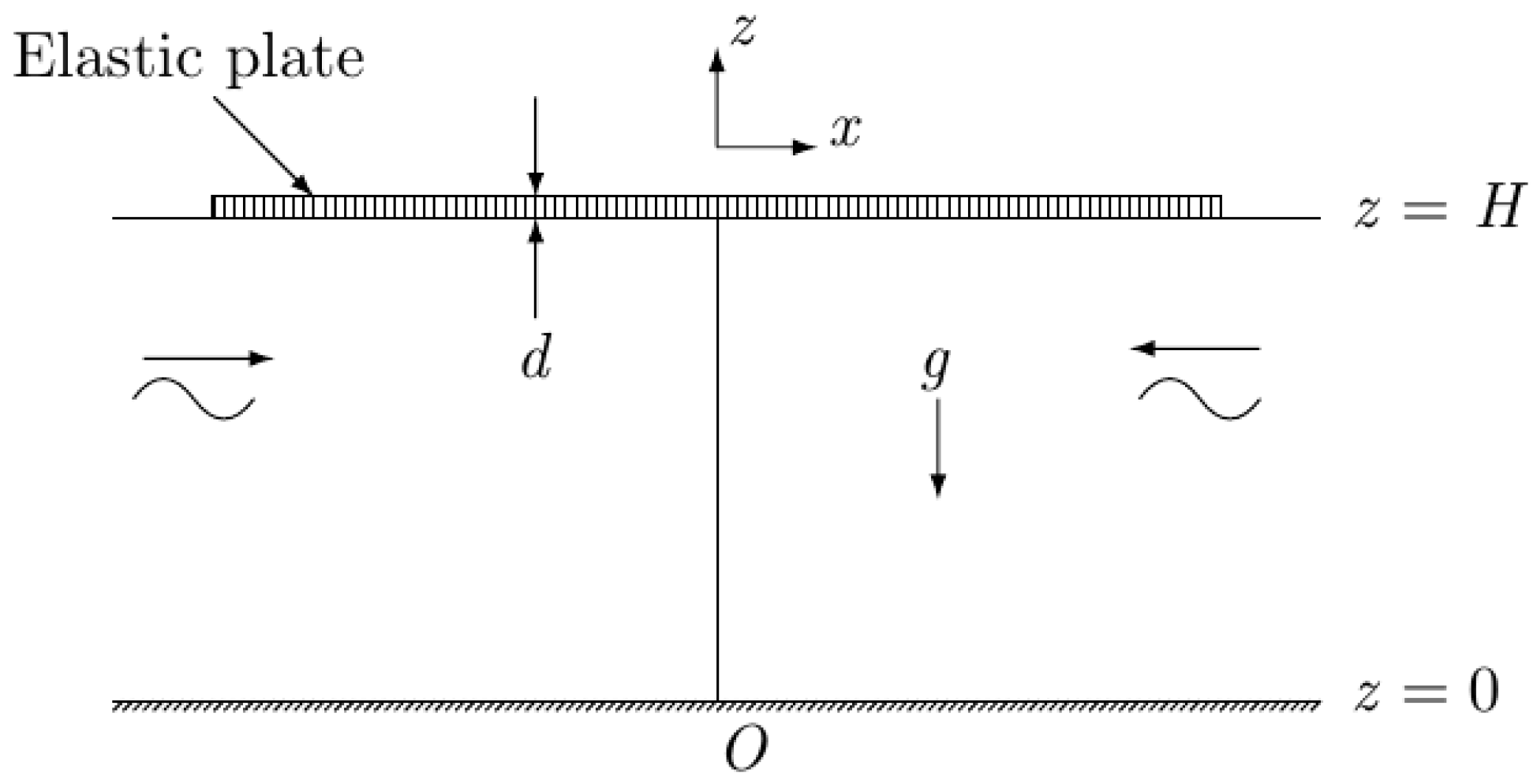
2. Mathematical Formulation
Consider a pair of nonlinear hydroelastic solitary waves propagating in the opposite directions through a finite channel. A Cartesian coordinate is selected to formulate the mathematical model, i.e., the
x-axis is proposed to lie along the horizontal direction, and the
z-axis is considered to lie along the vertical direction as shown in
Figure 1. A thin elastic plate is floating on the surface of water at
, and the horizontal bottom is located at
. Let
be the intensity of an underlying uniform current moving from left to right
. An opposing current is defined as that moving from the right to left
. The normal velocity of the governing fluid is taken as zero. The fluid is supposed to be incompressible, homogenous and inviscid, and the motion be irrotational. The velocity field in terms of potential function
satisfies
The bottom boundary condition at
is written as
The kinematic boundary condition at the water–plate interface (
) is defined as [
11,
29]
The dynamic boundary condition reads [
11,
29]
In the above equation,
is a uniform current,
g the gravitational acceleration,
the density of the fluid, and
the Bernoulli constant which is considered to be zero.
T is coefficient of surface tension of the fluid. The expression for pressure
consists on the Euler–Bernoulli beam theory which can be written as
where
is the flexural rigidity of the plate,
,
E Young’s modulus,
d constant thickness,
Poisson’s ratio, and
the uniform mass density of the elastic plate.
With the help of Equations (
1) and (
2), the potential function
can be describe using the Taylor series expansion at
, we have [
17]
where
Using Equation (
6), the kinematic and dynamic boundary condition can be obtained as
where
is a binomial coefficient. The asterisk in Equation (
9) indicates an inner vector product for the multiplication of even
j and odd
i.
Equations (
8) and (
9) can be simplified in the following form as
where
is the tangential velocity at the bottom of the channel.
3. Solution Methodology
We will employ the PLK method in the ensuing section. Let us introduce the following coordinate transformations in the wave frame, we have
where
k and
are the wave numbers of order unity for the right- and left-going waves, respectively;
with
is a dimensionless parameter that represents the order of magnitude of the wave amplitude.
C and
are the wave speeds of the right- and left-going solitary waves. Using the method of strained coordinates, we introduce the following transformation of wave frame coordinates with phase functions:
where
and
are the phase functions to be deduced in the perturbation analysis. The purpose of these functions is to obtain the asymptotic approximations which acquiesce us to analyze the phase changes due to a collision.
According to Ursell’s theory of shallow water waves, we consider the scaling of the horizontal wavelength as
. Although other values of
are also possible, i.e.,
, these values have some restriction in our present case. However, these values are used by different authors [
21,
24,
25] to derive various forms of the KdV equation in a two-layer fluid model but fail to give a KdV equation in our case. Later, Dai et al. [
27] used
to discuss the head-on collision among solitary waves propagating in a compressible Mooney–Rivlin elastic rod. The value of
plays a significant role and mainly depends upon physical and mathematical assumptions of the governing problem.
Let
where
is the non-dimensional elevation of the plate–fluid interface, and
is the undisturbed depth of the fluid. Considering the linear part of Equations (
11) and (
12), and assuming the linear solutions of
U and
take form of
, where
is the wave frequency, then we have the phase speed for the right-going wave as
and for the left-going wave it reads
where
The value
is the phase speed for pure gravity waves in shallow water of finite depth. The hydroelastic phase speed can be reduced for pure-gravity waves [
17] by taking
,
,
, and
.
For convenience, let us introduce a column vector
defined as
New variables are introduced in the form of the following power series:
where
and
(i.e.,
) are beneficial for removing the secular terms during the solution procedure;
a and
b are the amplitude factors.
5. Analytical Results
The series solutions in the preceding section are summarized in the following form.
The interfacial elevation at the water–plate interface can be written with the help of Equations (32) and (36), and we have
where
and
are defined in Equations (56) and (58).
The distortion profile can be calculated with the help of Equation (87). Therefore, the functions that are products of
and
must be removed. For this purpose, by taking
in Equation (87), the distortion profile at the water–plate interface can be written as
The maximum run-up
during the collision process at the water–plate interface can be obtained by taking
in Equation (87), namely
Following from Equations (32) and (36), the velocity at the bottom reads
Using Equations (40) and (65), the series solutions for the right- and left-going wave speeds are given by
The phase shifts for the right- and left-going wave read
where
,
,
, and
are given in Equations (50), (53), (74) and (79), respectively.
6. Graphical Analysis
This section describes the graphical behaviors of all the physical parameters involved in the governing two-dimensional hydroelastic wave problem. To determine the results in a more significant manner,
Figure 2,
Figure 3,
Figure 4,
Figure 5,
Figure 6,
Figure 7,
Figure 8,
Figure 9,
Figure 10,
Figure 11,
Figure 12,
Figure 13,
Figure 14,
Figure 15 and
Figure 16 depict the water–plate interface, distortion profile, wave speed, phase shift, and maximum run-up amplitude during the collision process. We consider the physical parameters, unless otherwise stated,
N m
−2,
m,
m s
−1,
m s
−2,
kg m
−3,
N m
−1,
m and
kg m
−3 for the graphical results. It is worth mentioning here that by taking
,
,
, and
in Equations (
3) and (
4), the present results reduce to those obtained by Su and Mirie [
17] for pure-gravity waves.
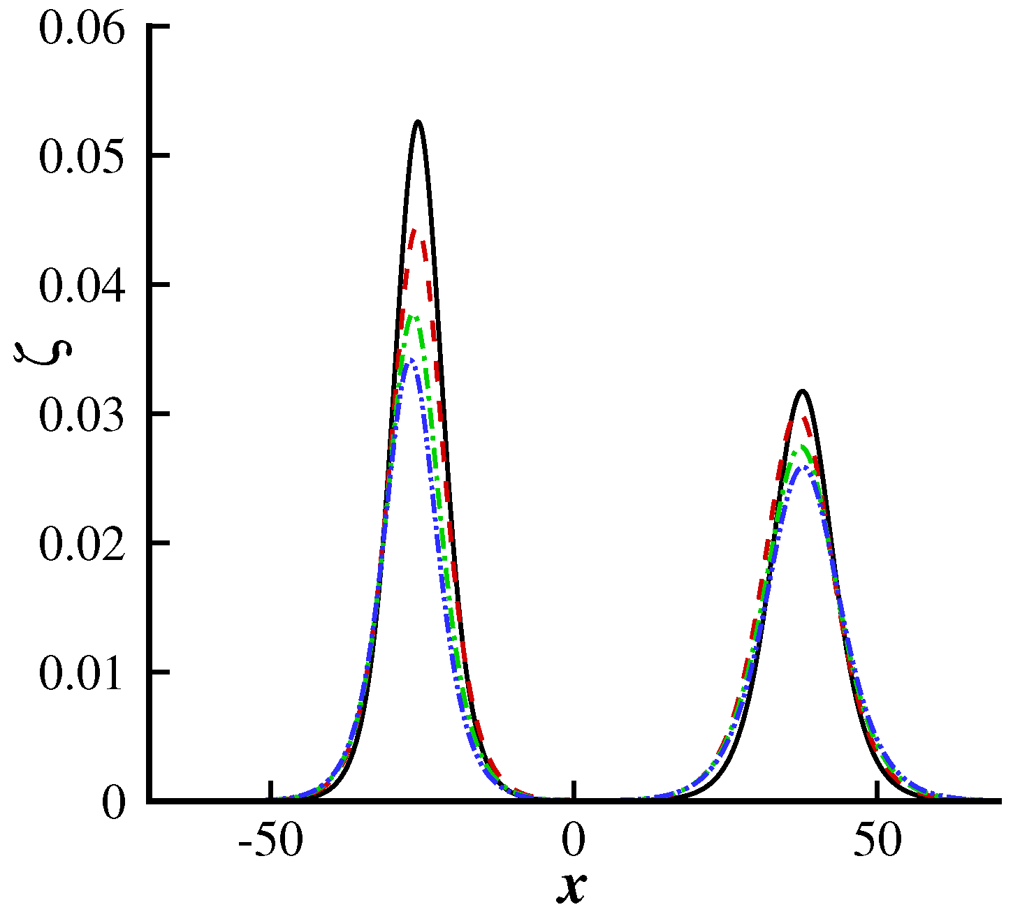
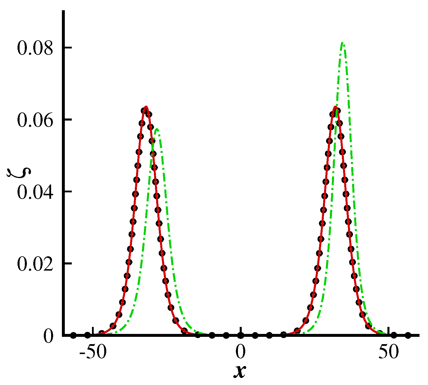
Figure 2 shows the wave profile for different values of
and
. When the effects of the elastic plate are taken into account, then significantly changes in the wave profile are observed. The parameter
is directly proportional to the plate thickness
d and Young’s modulus
E. When
and
increase, the plate becomes significantly stiffer, which produces a reactive force that opposes the deformation of hydroelastic waves.
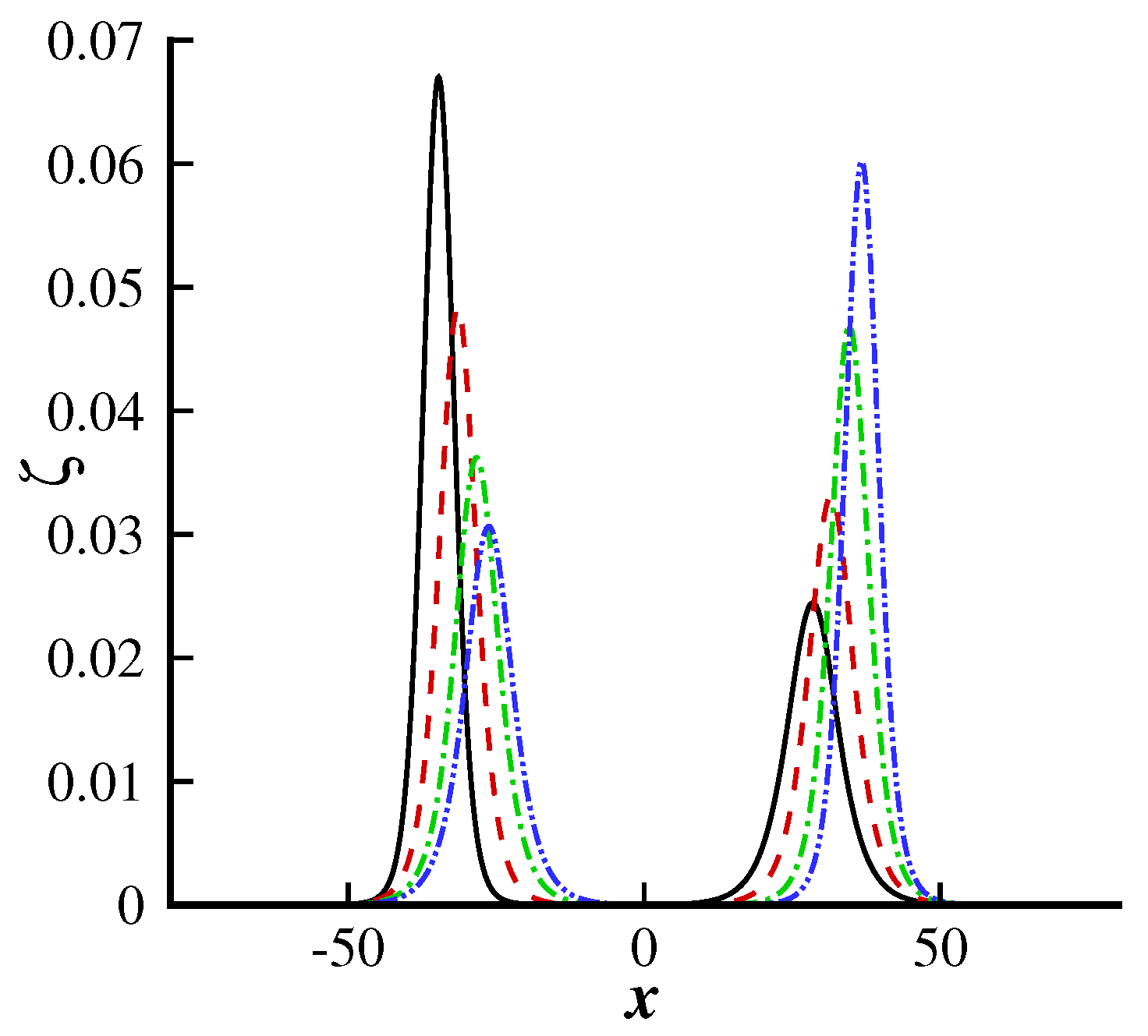
Figure 3 is plotted to see the effect of the current on the solitary wave profile. We can see from this figure that when the current is moving from right to left,
; then, the wavelength, amplitude and speed of the solitary waves are affected as shown in the region
. However, when
, a similar and converse behavior is found for the second solitary waves in the region
.
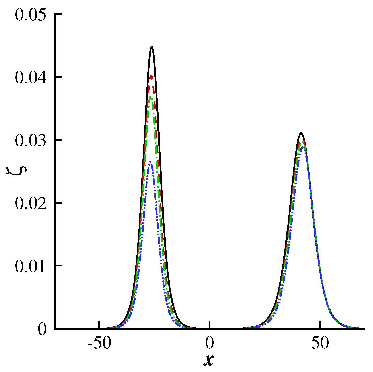
Figure 4 shows that an increment in the surface tension parameter
significantly diminishes the wave profile and that the wave profile before and after the collision process becomes narrower as the surface tension increases.
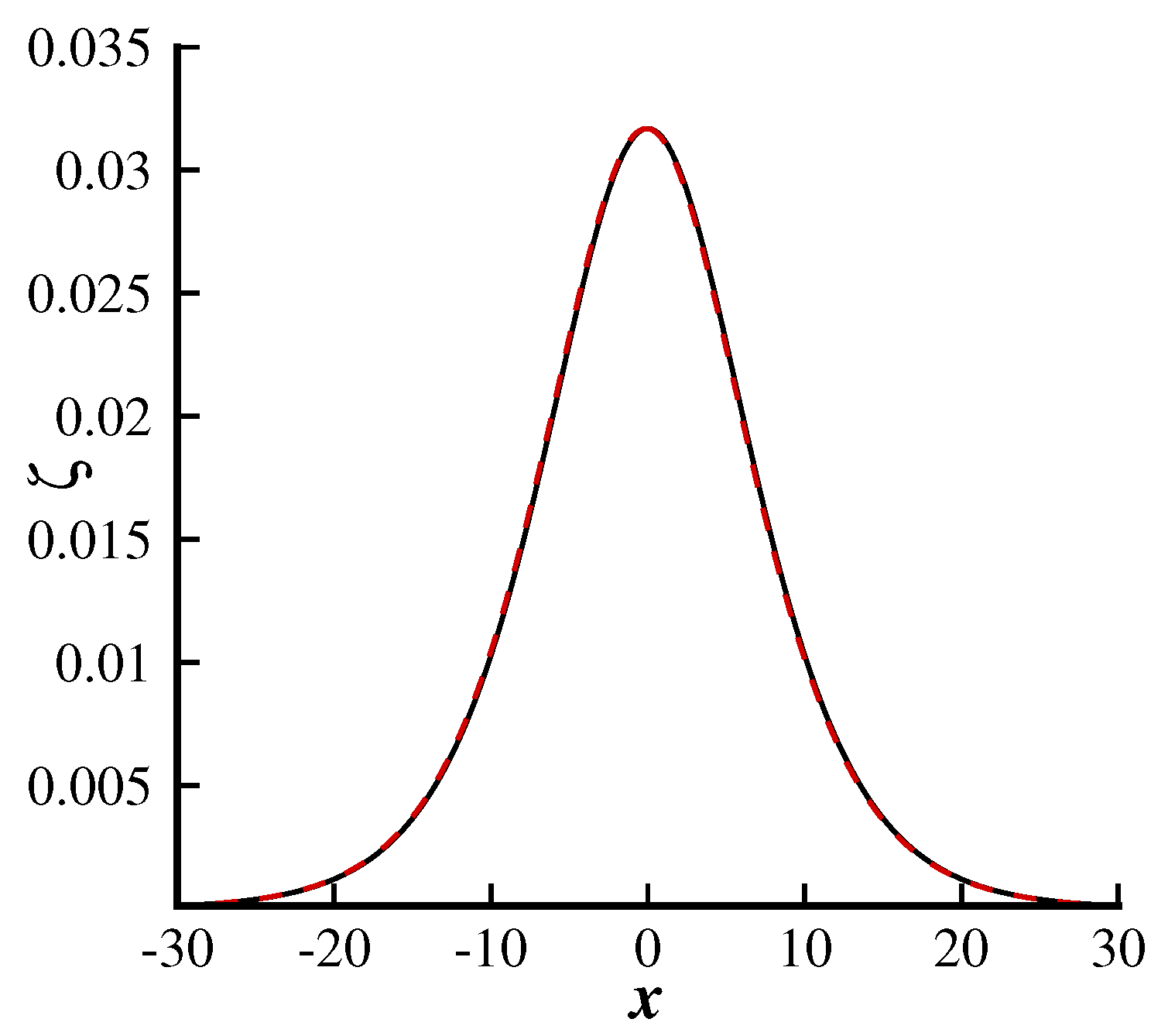
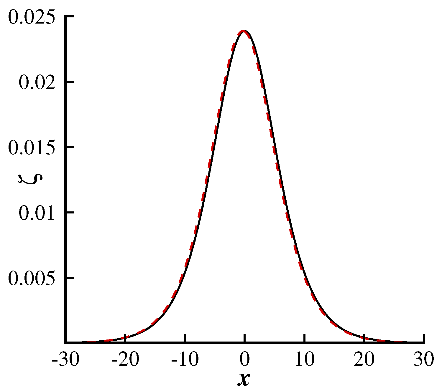
Figure 5 shows a graphical comparison with previously published results presented by Su and Mirie [
17]. We can observe that when
,
,
, and
, our results are in excellent agreement with those of Su and Mirie [
17] for pure gravity waves, which ensures the validity of the present results and the methodology used.
Figure 6 and
Figure 7 show the distortion profile during the head-on collision process for
and
. In both figures, we can see that before the collision process, the wave profile is similar for
and
. We can observe from these figures that during the collision process, the wave profile tilts backward in the direction of wave propagation. However, the wave profile remains symmetric before the collision process. Further, we can see that the wave profile is less affected by the following current
compared with the opposing current
. A similar behavior was also observed by Su and Mirie [
17] for pure gravity waves and Bhatti and Lu [
29] for nonlinear hydroelastic waves in the presence of a compressive force.
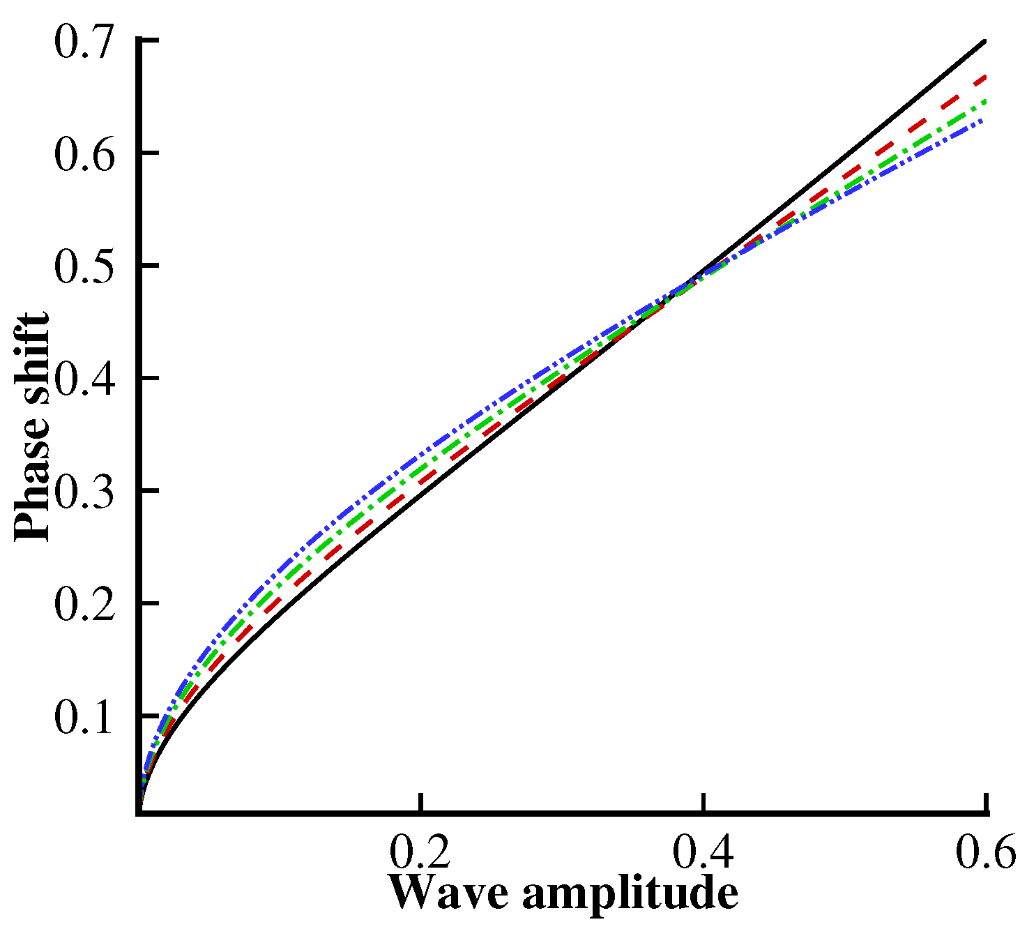
Figure 8,
Figure 9 and
Figure 10 are plotted for the phase shift profile against different values of
,
,
and
F. It can be noted from
Figure 8 that the initially phase shift profile increases due to the presence of the elastic plate, while its behavior becomes the opposite as the wave amplitude rises.
Figure 9 shows that the phase shift profile increases for higher values of the following current
, whereas its behavior is converse for higher values of the opposing current
.
Figure 10 shows the effects of the surface tension
on the phase shift profile. From this figure, we observe that the surface tension results are uniform throughout the domain, whereas the phase shift remarkably decreases due to a strong influence of the surface tension.
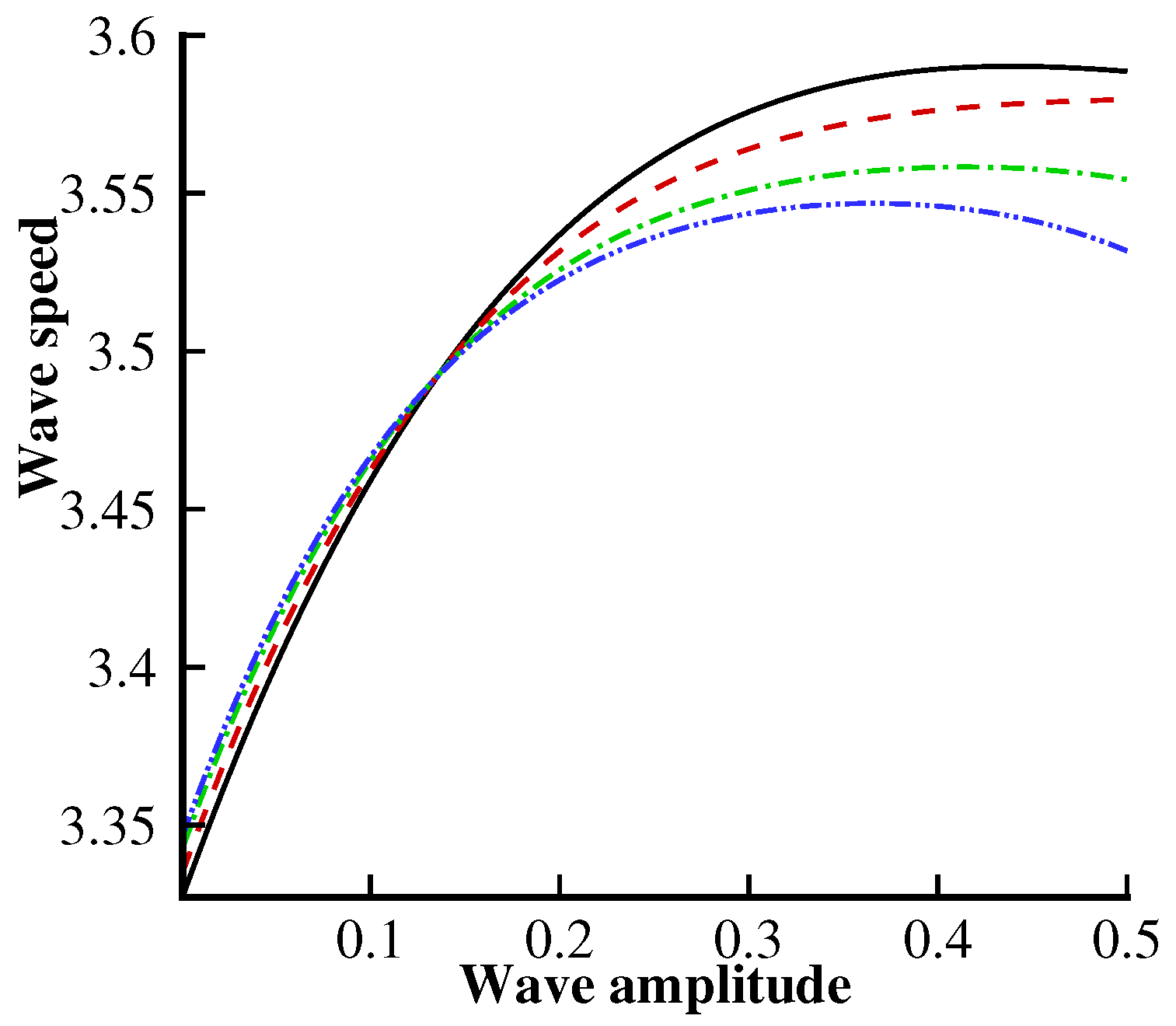
Figure 11,
Figure 12 and
Figure 13 show the variation of the wave speed with multiple values of
,
,
and
F. In
Figure 11, we can observe that the wave speed decreases significantly when
increases. Furthermore, the behavior of the left-going wave speed will be opposite to that of the right-going one.
Figure 12 is plotted to analyze the wave speed behavior for the left- and right-going solitary waves. In
Figure 12, we can easily observe that the left-going wave speed tends to diminish with the following current
, while the behavior is opposite for the right-going solitary wave. From
Figure 13, we note that the surface tension strongly influences the wave speed. We can see that the wave speed decreases due to an increment in the surface tension parameter
.
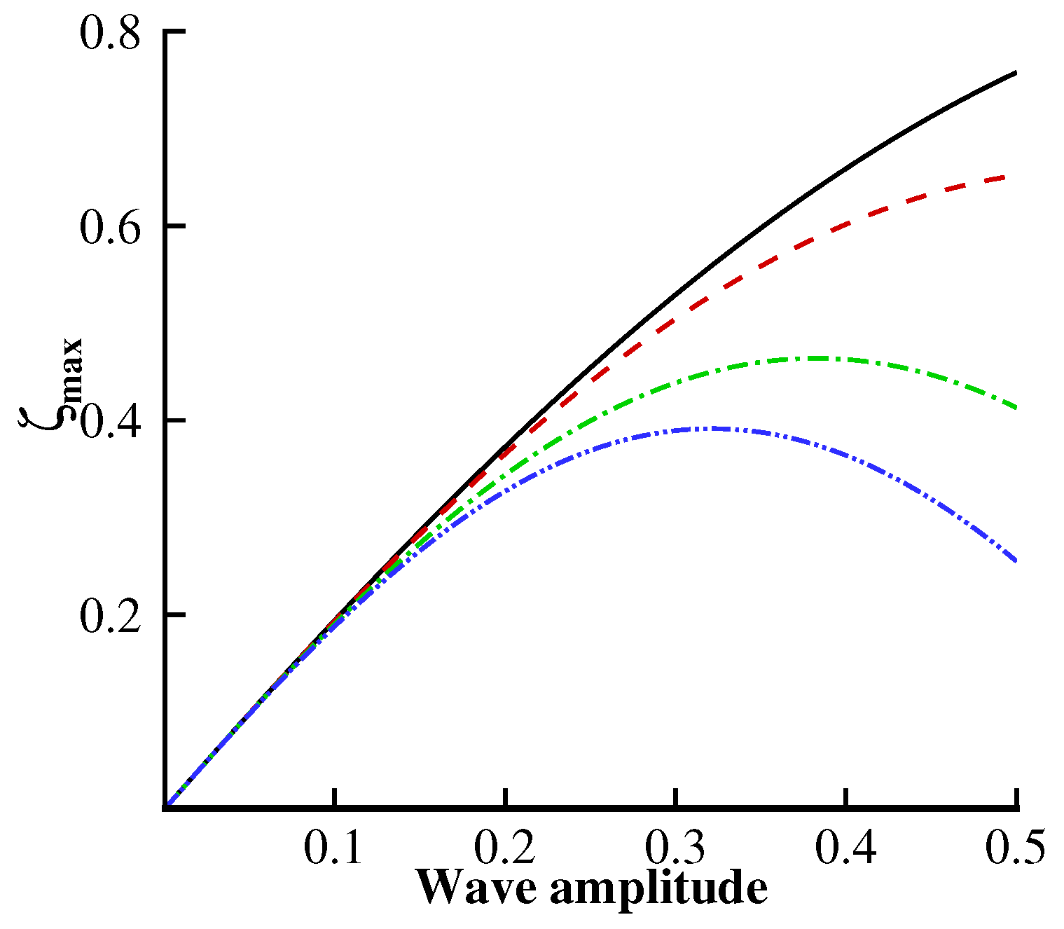
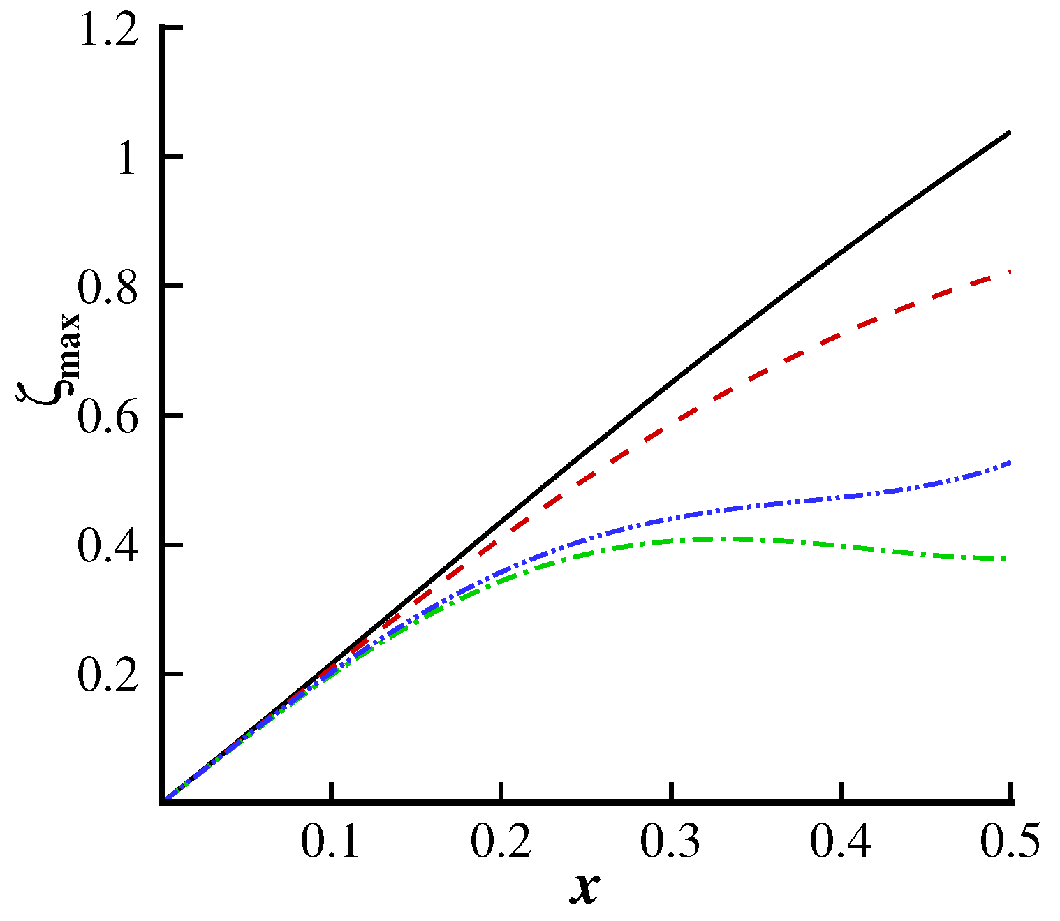
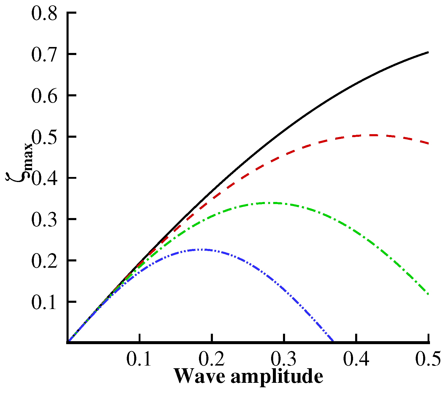
Figure 14,
Figure 15 and
Figure 16 present the variations in the maximum run-up during the collision process. It can be noted from
Figure 14 that the plate deflection creates an opposing force, which tends to resist the maximum run-up amplitude. Therefore, an increment of
or
tends to diminish the maximum run-up amplitude during the collision process. However, in
Figure 15, we can see that the maximum run-up amplitude increases for negative values of the current
, whereas its behavior is similar for higher values of the current when
. It can be observed from
Figure 16 that the surface tension parameter
significantly affects the wave speed compared with
,
F and
. An enhancement in the surface tension tends to reduce the maximum run-up amplitude.
7. Concluding Remarks
In this article, we analytically studied the behavior of a current in the head-on collision process between a pair of hydroelastic solitary waves propagating in the opposite directions. The Poincaré–Lighthill–Kuo method is successfully applied to obtain the solution for the governing nonlinear partial differential equations. The resulting solutions are presented up to the third-order approximation for right- and left-going solitary waves. The impact of different essential parameters is discussed with the help of graphs and presented mathematically for the water–plate interface, wave speed, phase shift, distortion profile, and maximum run-up amplitude during the collision process.
A graphical comparison with previously published results is also presented, and it is found that the present results are in excellent agreement, which ensures that the results for the hydroelastic wave problem are correct. It is also found that the presence of a thin elastic plate significantly reduces the amplitude of the wave profile. Furthermore, we noted that the presence of a current not only affects the wavelength and wave amplitude but also produces a remarkable effect on the wave speed. The phase shift markedly decreases due to the more significant influence of the elastic plate. It is also noted that the phase shift tends to increase for the following current, whereas its behavior is converse for the opposing current. The maximum run-up amplitude increases due to the strong influence of the following and opposing currents. It is observed that very small tilting occurs in the distortion profile during the collision process for positive values of the current, whereas greater tilting in the wave profile is seen for negative current values.


