Fractional Telegraph Equation and Its Solution by Natural Transform Decomposition Method

Abstract

In this work, the natural transform decomposition method (NTDM) is applied to solve the linear and nonlinear fractional telegraph equations. This method is a combined form of the natural transform and the Adomian decomposition methods. In addition, we prove the convergence of our method. Finally, three examples have been employed to illustrate the preciseness and effectiveness of the proposed method.

1. Introduction

The fractional calculus (non-integer) plays an important role in applied mathematics and other fields such as science, physics and engineering. It describes the smallest details of natural phenomena, which is better than using a calculus integer. In [1] the fractional telegraph equation is obtained from the classical telegraph equation by replacing the second-order distance derivative with the fractional derivative $\left(0<\alpha \le 2\right)$ given to it. The telegraph equation describes the signal propagation of an electrical signal in transmission cable lines in general. Recently, many researchers and engineers have done excellent work to solve the fractional telegraph equation by different methods, such as the Laplace transform method [2], Laplace transform variational iteration method [3], double Laplace transform method [4], variational iteration method [5], Adomian decomposition method [6], Mixture of a new integral transform and homotopy perturbation method (HPM) [7], homotopy analysis method (HAM) [8], Chebyshev tau method [9], and the method of separating variables [10]. The natural transform Adomian decomposition method (NTDM) is a combination of the natural transform method and Adomian decomposition method. The main aim of this article is to use the (NTDM) to obtain the approximate solution of linear and nonlinear fractional telegraph equations. The natural transform Adomian decomposition method is a sturdy mathematical method for solving linear and nonlinear fractional telegraph equation and is an amelioration of the existing methods.

2. Preliminaries

Definition 1

([11]). The Adomian decomposition method is defined as

$$A_n=\frac{1}{n!}\frac{d^n}{d{\lambda }^n}{\left[F\left(\sum _{i=1}^n{\psi }_i{\lambda }^i\right)\right]}_{\lambda =0},n=0,1,2,\dots$$

(1)

where the function F $\left(\psi \right)$ is a nonlinear term and $\lambda$ a formal parameter.

Definition 2

([12]). The natural transform of a function $f\left(t\right)>0$ and $f\left(t\right)=0$ for $t<0$ is defined by

$${\mathbb{N}}^{+}\left[f\left(t\right)\right]=R(s,u)=\frac{1}{u}{\int }_0^{\infty }{e}^{\frac{-st}{u}}f\left(t\right)dt;s,u>0$$

(2)

where s and u are the transform variables.

Definition 3

([12,13]). The inverse natural transform of a function is defined by

$${\mathbb{N}}^{-}\left[R(s,u)\right]=f\left(t\right)=\frac{1}{2\pi i}{\int }_{c-i\infty }^{c+i\infty }{e}^{\frac{st}{u}}R(s,u)ds$$

Definition 4

([14]).The natural transform of $\frac{{\partial }^{\alpha }f(x,t)}{\partial t^{\alpha }}$ w.r.t $\left(t\right)$ can be calculated as

$${\mathbb{N}}^{+}\left[\frac{{\partial }^{\alpha }f(x,t)}{\partial t^{\alpha }}\right]=\frac{s^{\alpha }}{u^{\alpha }}R(s,u)-\sum _{k=0}^{n-1}\frac{s^{\alpha -k-1}}{u^{\alpha -k}}\left[\frac{{\partial }^{\alpha }f(x,0)}{\partial t^{\alpha }}\right]$$

(3)

Definition 5

([14]). The natural transform of Mittag-Leffler function $E_{\alpha ,\beta }$ is defined as follows

$${\mathbb{N}}^{+}\left[f(x,t)\right]={\int }_0^{\infty }{e}^{-st}f(x,ut)dt=\sum _{k=0}^{\infty }\frac{u^{k+1}\Gamma (k+\beta )}{s^{k+1}\Gamma (\alpha k+\beta )}$$

(4)

Definition 6

([15]).A two parameter function of the Mittag-Leffler type is defined by the series expansion

$$E_{\alpha ,\beta }\left(z\right)=\sum _{k=0}^{\infty }\frac{z^k}{\Gamma (\alpha k+\beta )},(\alpha >0,\beta >0)$$

(5)

3. Natural Transform Adomian Decomposition Method Linear and Nonlinear Telegraph Equations (NTADM)

In this section, we will study two problems as follows:

First Problem: linear fractional telegraph equations

In this part, we derive the main idea of the natural transform decomposition method to find the general solution for linear fractional telegraph equations.

We consider the following general multiterm fractional telegraph equation

$$\begin{array}{c}\frac{{\partial }^{\alpha }\psi (x,t)}{\partial t^{\alpha }}=\frac{{\partial }^2\psi (x,t)}{\partial x^2}-\frac{\partial \psi (x,t)}{\partial t}-\psi (x,t)+h(x,t),\\ 0<\alpha \le 2\mathrm{and}x,t\ge 0\end{array}$$

(6)

subject to

$$\psi (x,0)=f_1\left(x\right)\mathrm{and}{\psi }_t(x,0)=f_2\left(x\right)$$

(7)

where $h(x,t)$ is given function. The new technique of natural transform Adomian decomposition is based on the following steps. By applying the definition of natural transform to Equation (6), we get

$$\begin{array}{c}\frac{s^{\alpha }}{u^{\alpha }}R(x,s,u)-\frac{s^{\alpha -1}}{u^{\alpha }}\psi (x,0)-\frac{s^{\alpha -2}}{u^{\alpha -1}}{\psi }_t(x,0)={\mathbb{N}}^{+}\left[\frac{{\partial }^2\psi (x,t)}{\partial x^2}-\frac{\partial \psi (x,t)}{\partial t}-\psi (x,t)+h(x,t)\right],\hfill \end{array}$$

(8)

substituting the initial conditions Equation (7) into Equation (8), we obtain

$$\begin{array}{c}R(x,s,u)=\frac{1}{s}{f}_1\left(x\right)+\frac{u}{s^2}{f}_2\left(x\right)+\frac{u^{\alpha }}{s^{\alpha }}{\mathbb{N}}^{+}\left[\frac{{\partial }^2\psi (x,t)}{\partial x^2}-\frac{\partial \psi (x,t)}{\partial t}-\psi (x,t)+h(x,t)\right].\hfill \end{array}$$

(9)

Now, implementing the inverse natural transform for Equation (9) we obtain the general solution of Equation (6) as follows:

$$\psi (x,t)=\Phi (x,t)+{\mathbb{N}}^{-1}\left[\frac{u^{\alpha }}{s^{\alpha }}{\mathbb{N}}^{+}\left[\frac{{\partial }^2\psi (x,t)}{\partial x^2}-\frac{\partial \psi (x,t)}{\partial t}-\psi (x,t)\right]\right],$$

(10)

where

$$\Phi (x,t)={\mathbb{N}}^{-1}\left[f_1\left(x\right)+t{f}_2\left(x\right)+\frac{u^{\alpha }}{s^{\alpha }}{N}^{+}\left[h(x,t)\right]\right],$$

(11)

the natural transform decomposition method defined the solution of $\psi (x,t)$ by the infinite series

$$\psi (x,t)=\sum _{n=0}^{\infty }{\psi }_n(x,t).$$

(12)

The solution of Equation (10) is given by

$$\sum _{n=0}^{\infty }{\psi }_n(x,t)=\Phi (x,t)+{\mathbb{N}}^{-1}\left[\frac{u^{\alpha }}{s^{\alpha }}{\mathbb{N}}^{+}\left[\sum _{n=0}^{\infty }\frac{{\partial }^2{\psi }_n(x,t)}{\partial x^2}-\sum _{n=0}^{\infty }\frac{\partial {\psi }_n(x,t)}{\partial t}-\sum _{n=0}^{\infty }{\psi }_n(x,t)\right]\right].$$

(13)

Here we assume that the inverse natural transform of each term in the right side of Equation (9) exists. The initial term

$${\psi }_0(x,t)=\Phi (x,t),$$

(14)

consequently, the first few components can be written as

$$\begin{array}{c}{\psi }_1(x,t)={\mathbb{N}}^{-1}\left[\frac{u^{\alpha }}{s^{\alpha }}{\mathbb{N}}^{+}\left[\frac{{\partial }^2{\psi }_0(x,t)}{\partial x^2}-\frac{\partial {\psi }_0(x,t)}{\partial t}-{\psi }_0(x,t)\right]\right]\hfill \\ {\psi }_2(x,t)={\mathbb{N}}^{-1}\left[\frac{u^{\alpha }}{s^{\alpha }}{\mathbb{N}}^{+}\left[\frac{{\partial }^2{\psi }_1(x,t)}{\partial x^2}-\frac{\partial {\psi }_1(x,t)}{\partial t}-{\psi }_1(x,t)\right]\right]\hfill \\ {\psi }_3(x,t)={\mathbb{N}}^{-1}\left[\frac{u^{\alpha }}{s^{\alpha }}{\mathbb{N}}^{+}\left[\frac{{\partial }^2{\psi }_2(x,t)}{\partial x^2}-\frac{\partial {\psi }_2(x,t)}{\partial t}-{\psi }_2(x,t)\right]\right]\hfill \\ .\hfill \\ .\hfill \\ .\hfill \end{array}$$

(15)

then we have

$${\psi }_{n+1}(x,t)={\mathbb{N}}^{-1}\left[\frac{u^{\alpha }}{s^{\alpha }}{\mathbb{N}}^{+}\left[\frac{{\partial }^2{\psi }_n(x,t)}{\partial x^2}-\frac{\partial {\psi }_n(x,t)}{\partial t}-{\psi }_n(x,t)\right]\right],n\ge 0$$

(16)

Second Problem Nonlinear fractional telegraph equation:

We consider the general form of nonlinear fractional telegraph equation:

$$\begin{array}{c}\frac{{\partial }^{\alpha }\psi (x,t)}{\partial t^{\alpha }}=\frac{{\partial }^2\psi (x,t)}{\partial x^2}-\frac{\partial \psi (x,t)}{\partial t}-N\psi (x,t)+h(x,t),\\ 0<\alpha \le 2\mathrm{and}x,t\ge 0\end{array}$$

(17)

with the initial conditions

$$\psi (x,0)=g_1\left(x\right)\mathrm{and}{\psi }_t(x,0)=g_2\left(x\right),$$

(18)

where N is a nonlinear, $h(x,t)$ is a source term. By applying the definition of natural transform for Equation (17), we have

$$\begin{array}{c}\frac{s^{\alpha }}{u^{\alpha }}R(x,s,u)-\frac{s^{\alpha -1}}{u^{\alpha }}\psi (x,0)-\frac{s^{\alpha -2}}{u^{\alpha -1}}{\psi }_t(x,0)={\mathbb{N}}^{+}\left[\frac{{\partial }^2\psi (x,t)}{\partial x^2}-\frac{\partial \psi (x,t)}{\partial t}-N\psi (x,t)+h(x,t)\right],\hfill \end{array}$$

(19)

by substituting initial conditions Equation (18) into Equation (19), we obtain

$$R(x,s,u)=\frac{1}{s}{g}_1\left(x\right)+\frac{u}{s^2}{g}_2\left(x\right)+\frac{u^{\alpha }}{s^{\alpha }}{\mathbb{N}}^{+}\left[\frac{{\partial }^2\psi (x,t)}{\partial x^2}-\frac{\partial \psi (x,t)}{\partial t}-N\psi (x,t)+h(x,t)\right].$$

(20)

Now, implementing the inverse natural transform for Equation (20), we obtain the general solution of Equation (17) in the form of,

$$\psi (x,t)=\Phi (x,t)+{\mathbb{N}}^{-1}\left[\frac{u^{\alpha }}{s^{\alpha }}{\mathbb{N}}^{+}\left[\frac{{\partial }^2\psi (x,t)}{\partial t^2}-\frac{\partial \psi (x,t)}{\partial t}-N\psi (x,t)\right]\right],$$

(21)

where

$$\Phi (x,t)={\mathbb{N}}^{-1}\left[g_1\left(x\right)+t{g}_2\left(x\right)+\frac{u^{\alpha }}{s^{\alpha }}{\mathbb{N}}^{+}\left[h(x,t)\right]\right],$$

(22)

here we assume that the inverse natural transform of each term in the right side of Equation (22) exists. The natural transform decomposition method consists of calculating the solution in a series form

$$\psi (x,t)=\sum _{n=0}^{\infty }{\psi }_n(x,t),$$

(23)

the nonlinear term $N\psi (x,t)$ becomes

$$N\psi (x,t)=\sum _{n=0}^{\infty }{A}_n,$$

(24)

where $A_n$ defined by Equation (1). By substituting Equations (23) and (24) into Equation (21) we get

$$\sum _{n=0}^{\infty }{\psi }_n(x,t)=\Phi (x,t)+{\mathbb{N}}^{-1}\left[\frac{u^{\alpha }}{s^{\alpha }}{\mathbb{N}}^{+}\left[\sum _{n=0}^{\infty }\frac{{\partial }^2{\psi }_n(x,t)}{\partial x^2}-\sum _{n=0}^{\infty }\frac{\partial {\psi }_n(x,t)}{\partial t}-\sum _{n=0}^{\infty }{A}_n\right]\right],$$

(25)

by using the recursive relation

$${\psi }_0(x,t)=\Phi (x,t)$$

(26)

consequently, the first few components can be written as

$$\begin{array}{c}{\psi }_1(x,t)={\mathbb{N}}^{-1}\left[\frac{u^{\alpha }}{s^{\alpha }}{\mathbb{N}}^{+}\left[\frac{{\partial }^2{\psi }_0(x,t)}{\partial x^2}-\frac{\partial {\psi }_0(x,t)}{\partial t}-A_0\right]\right]\hfill \\ {\psi }_2(x,t)={\mathbb{N}}^{-1}\left[\frac{u^{\alpha }}{s^{\alpha }}{\mathbb{N}}^{+1}\left[\frac{{\partial }^2{\psi }_1(x,t)}{\partial x^2}-\frac{\partial {\psi }_1(x,t)}{\partial t}-A_1\right]\right]\hfill \\ {\psi }_3(x,t)={\mathbb{N}}^{-1}\left[\frac{u^{\alpha }}{s^{\alpha }}{\mathbb{N}}^{+}\left[\frac{{\partial }^2{\psi }_2(x,t)}{\partial x^2}-\frac{\partial {\psi }_2(x,t)}{\partial t}-A_2\right]\right],\hfill \\ .\hfill \\ .\hfill \\ .\hfill \end{array}$$

(27)

then we have

$${\psi }_{n+1}(x,t)={\mathbb{N}}^{-1}\left[\frac{u^{\alpha }}{p^{\alpha }}{\mathbb{N}}^{+}\left[\frac{{\partial }^2{\psi }_n(x,t)}{\partial t^2}+\frac{\partial {\psi }_n(x,t)}{\partial t}+A_n\right]\right],n\ge 0$$

(28)

the solution ${\psi }_n(x,t)$ can be written as convergent series

$$\psi (x,t)=\sum _{n=0}^{\infty }{\psi }_n(x,t).$$

(29)

4. Convergence Analysis

In this section, the sufficient condition that guarantees existence of a unique solution is introduced and we discuss the convergence of the solution.

In next theorem we follow [16]

Theorem 1.

(Uniqueness theorem): Equation (28) has a unique solution whenever $0<\epsilon <1$ where $\epsilon =\frac{(L_1+L_2+L_3)t^{\alpha +1}}{(\alpha -1)!}$

Proof of Theorem 1.

Let $E=\left(C\left[I\right],∥.∥\right)$ be the Banach space of all continuous functions on $I=\left[0,T\right]$ with the norm $∥.∥$, we define a mapping $F:E\to E$ where

$${\psi }_{n+1}(x,t)=\Phi (x,t)+{\mathbb{N}}^{-1}\left[\frac{u^{\alpha }}{s^{\alpha }}{\mathbb{N}}^{+}\left[L\left[{\psi }_n(x,t)\right]+M\left[{\psi }_n(x,t)\right]+N\left[{\psi }_n(x,t)\right]\right]\right],n\ge 0$$

where $L\left[\psi (x,t)\right]\equiv \frac{{\partial }^2\psi (x,t)}{\partial x^2}andM\left[\psi (x,t)\right]\equiv \frac{\partial \psi (x,t)}{\partial t}.$ Now suppose $M\left[\psi (x,t)\right]$ and $L\left[\psi (x,t)\right]$ is also Lipschitzian with $\left|M\psi -M\stackrel{⌢}{\psi }\right|<L_1\left|\psi -\stackrel{⌢}{\psi }\right|$ and $\left|L\psi -L\stackrel{⌢}{\psi }\right|<L_2\left|\psi -\stackrel{⌢}{\psi }\right|$ where $L_1$ and $L_2$ is Lipschitz constant respectively and $\psi$,$\stackrel{⌢}{\psi }$ is different values of the function.

$$\begin{array}{cc}∥F\psi -F\stackrel{⌢}{\psi }∥& =\underset{t\in I}{\max }\left|\begin{array}{c}{\mathbb{N}}^{-1}\left[\frac{u^{\alpha }}{s^{\alpha }}{\mathbb{N}}^{+}\left[L\left[\psi (x,t)\right]+M\left[\psi (x,t)\right]+N\left[\psi (x,t)\right]\right]\right]\\ -{\mathbb{N}}^{-1}\left[\frac{u^{\alpha }}{s^{\alpha }}{\mathbb{N}}^{+}\left[L\left[\stackrel{⌢}{\psi }(x,t)\right]+M\left[\stackrel{⌢}{\psi }(x,t)\right]+N\left[\stackrel{⌢}{\psi }(x,t)\right]\right]\right]\end{array}\right|,\\ & \le \underset{t\in I}{\max }\left|\begin{array}{c}{\mathbb{N}}^{-1}\left[\frac{u^{\alpha }}{p^{\alpha }}{\mathbb{N}}^{+}\left[L\left[\psi (x,t)\right]-L\left[\stackrel{⌢}{\psi }(x,t)\right]\right]\right]\\ +{\mathbb{N}}^{-1}\left[\frac{u^{\alpha }}{s^{\alpha }}{\mathbb{N}}^{+}\left[M\left[\psi (x,t)\right]-M\left[\stackrel{⌢}{\psi }(x,t)\right]\right]\right]\\ +{\mathbb{N}}^{-1}\left[\frac{u^{\alpha }}{s^{\alpha }}{\mathbb{N}}^{+}\left[N\left[\psi (x,t)\right]-N\left[\stackrel{⌢}{\psi }(x,t)\right]\right]\right]\end{array}\right|,\hfill \\ & \le \underset{t\in I}{\max }\left[\begin{array}{c}{L}_1{\mathbb{N}}^{-1}\left[\frac{u^{\alpha }}{s^{\alpha }}{\mathbb{N}}^{+}\left|\psi (x,t)-\stackrel{⌢}{\psi }(x,t)\right|\right]\\ +L_2{\mathbb{N}}^{-1}\left[\frac{u^{\alpha }}{s^{\alpha }}{\mathbb{N}}^{+}\left|\psi (x,t)-\stackrel{⌢}{\psi }(x,t)\right|\right]\\ +L_3{\mathbb{N}}^{-1}\left[\frac{u^{\alpha }}{s^{\alpha }}{\mathbb{N}}^{+}\left|\psi (x,t)-\stackrel{⌢}{\psi }(x,t)\right|\right]\end{array}\right],\hfill \\ & \le \underset{t\in I}{\max }\left(L_1+L_2+L_3\right)\left[{\mathbb{N}}^{-1}\left[\frac{u^{\alpha }}{s^{\alpha }}{\mathbb{N}}^{+}\left|\psi (x,t)-\stackrel{⌢}{\psi }(x,t)\right|\right]\right],\hfill \\ & \le \left(L_1+L_2+L_3\right)\left[{\mathbb{N}}^{-1}\left[\frac{u^{\alpha }}{s^{\alpha }}{\mathbb{N}}^{+}∥\psi (x,t)-\stackrel{⌢}{\psi }(x,t)∥\right]\right],\hfill \\ & =\frac{\left(L_1+L_2+L_3\right)t^{(\alpha -1)}}{(\alpha -1)!}∥\psi (x,t)-\stackrel{⌢}{\psi }(x,t)∥.\hfill \end{array}$$

Under the condition $0<\epsilon <1$, the mapping is contraction. Therefore, by Banach fixed point theorem for contraction, there exists a unique solution to Equation (29). This ends the proof of Theorem 1. ☐

Theorem 2.

(Convergence Theorem): The solution of Equations (6) and (18) in general forum will be convergence.

Proof of Theorem 2.

Let $S_n$ be the $n^{th}$ partial sum, i.e., $S_n={\sum }_{i=0}^n{\psi }_i(x,t)$. We shall prove that $\left\{S_n\right\}$ is a Cauchy sequence in Banach space E. By using a new formulation of Adomian polynomials we get

$$\begin{array}{c}lR\left(S_n\right)={\stackrel{⌢}{A}}_n+\sum _{r=0}^{n-1}{\stackrel{⌢}{A}}_r\hfill \\ N\left(S_n\right)={\stackrel{⌢}{A}}_n+\sum _{c=0}^{n-1}{\stackrel{⌢}{A}}_c\hfill \\ ∥S_n-S_m∥=\underset{t\in I}{\max }\left|S_n-S_m\right|=\underset{t\in I}{\max }\left|\sum _{i=m+1}^n{\stackrel{⌢}{\psi }}_i(x,t)\right|, p=1,2,3,...\hfill \end{array}$$

$$\begin{array}{c}\le \underset{t\in I}{\max }\left|\begin{array}{c}{\mathbb{N}}^{-1}\left[\frac{u^{\alpha }}{s^{\alpha }}{\mathbb{N}}^{+}\left[\sum _{i=m+1}^{n}L\left[{\psi }_{n-1}(x,t)\right]\right]\right]\\ +{\mathbb{N}}^{-1}\left[\frac{u^{\alpha }}{s^{\alpha }}{\mathbb{N}}^{+}\left[\sum _{i=m+1}^{n}M\left[{\psi }_{n-1}(x,t)\right]\right]\right]\\ +{\mathbb{N}}^{-1}\left[\frac{u^{\alpha }}{s^{\alpha }}{\mathbb{N}}^{+}\left[\sum _{i=m+1}^n{A}_{n-1}(x,t)\right]\right]\end{array}\right|,\hfill \\ =\underset{t\in I}{\max }\left|\begin{array}{c}{\mathbb{N}}^{-1}\left[\frac{u^{\alpha }}{s^{\alpha }}{\mathbb{N}}^{+}\left[\sum _{i=m}^{n-1}L\left[{\psi }_n(x,t)\right]\right]\right]\\ +{\mathbb{N}}^{-1}\left[\frac{u^{\alpha }}{s^{\alpha }}{\mathbb{N}}^{+}\left[\sum _{i=m}^{n-1}M\left[{\psi }_n(x,t)\right]\right]\right]\\ +{\mathbb{N}}^{-1}\left[\frac{u^{\alpha }}{s^{\alpha }}{\mathbb{N}}^{+}\left[\sum _{i=m+1}^n{A}_n(x,t)\right]\right]\end{array}\right|,\hfill \\ \le \underset{t\in I}{\max }\left|\begin{array}{c}{\mathbb{N}}^{-1}\left[\frac{u^{\alpha }}{s^{\alpha }}{\mathbb{N}}^{+}\left[\sum _{i=m}^{n-1}L\left(S_{n-1}\right)-L\left(S_{m-1}\right)\right]\right]\\ +{\mathbb{N}}^{-1}\left[\frac{u^{\alpha }}{s^{\alpha }}{\mathbb{N}}^{+}\left[\sum _{i=m}^{n-1}M\left(S_{n-1}\right)-M\left(S_{m-1}\right)\right]\right]\\ +{\mathbb{N}}^{-1}\left[\frac{u^{\alpha }}{s^{\alpha }}{\mathbb{N}}^{+}\left[\sum _{i=m+1}^{n}N\left(S_{n-1}\right)-N\left(S_{m-1}\right)\right]\right]\end{array}\right|,\hfill \\ \le \underset{t\in I}{\max }\left|\begin{array}{c}{\mathbb{N}}^{-1}\left[\frac{u^{\alpha }}{s^{\alpha }}{\mathbb{N}}^{+}\left[L\left(S_{n-1}\right)-L\left(S_{m-1}\right)\right]\right]\\ +{\mathbb{N}}^{-1}\left[\frac{u^{\alpha }}{s^{\alpha }}{\mathbb{N}}^{+}\left[M\left(S_{n-1}\right)-R\left(S_{m-1}\right)\right]\right]\\ +{\mathbb{N}}^{-1}\left[\frac{u^{\alpha }}{s^{\alpha }}{\mathbb{N}}^{+}\left[N\left(S_{n-1}\right)-N\left(S_{m-1}\right)\right]\right]\end{array}\right|,\hfill \\ \le L_1\underset{t\in I}{\max }{\mathbb{N}}^{-1}\left|\left[\frac{u^{\alpha }}{s^{\alpha }}{\mathbb{N}}^{+}\left[\left(S_{n-1}\right)-\left(S_{m-1}\right)\right]\right]\right|,\hfill \\ +L_2\underset{t\in I}{\max }{\mathbb{N}}^{-1}\left|\left[\frac{u^{\alpha }}{s^{\alpha }}{\mathbb{N}}^{+}\left[\left(S_{n-1}\right)-\left(S_{m-1}\right)\right]\right]\right|,\hfill \\ +L_3\underset{t\in I}{\max }{\mathbb{N}}^{-1}\left|\left[\frac{u^{\alpha }}{s^{\alpha }}{\mathbb{N}}^{+}\left[\left(S_{n-1}\right)-\left(S_{m-1}\right)\right]\right]\right|.\hfill \end{array}$$

$$=\frac{(L_1+L_2+L_3)t^{(\alpha -1)}}{(\alpha -1)!}∥S_{n-1}+S_{m-1}∥$$

Let $n=m+1;$ then

$$∥S_{m+1}-S_m∥\le \epsilon ∥S_m-S_{m-1}∥\le {\epsilon }^2∥S_{m-1}-S_{m-2}∥\le \dots \le {\epsilon }^m∥S_1-S_0∥.$$

where $\epsilon =\frac{(L_1+L_2+L_3)t^{(\alpha -1)}}{(\alpha -1)!}$ similarly, we have, from the triangle inequality we have

$$∥S_n-S_m∥\le ∥S_{m+1}-S_m∥+∥S_{m+2}-S_{m+1}∥+\dots +∥S_n-S_{n-1}∥,$$

$$\le \left[{\epsilon }^m+{\epsilon }^{m+1}+\dots +{\epsilon }^{n-1}\right]\le ∥S_1+S_0∥,$$

$$\le {\epsilon }^m\left(\frac{1-{\epsilon }^{n-m}}{\epsilon }\right)∥{\psi }_1∥,$$

since $0<\epsilon <1$ we have $\left(1-{\epsilon }^{n-m}\right)<1$: then,

$$∥S_n-S_m∥\le \frac{{\epsilon }^m}{1-\epsilon }\underset{t\in I}{\max }∥{\psi }_1∥.$$

However, $\left|{\psi }_1\right|<\infty$ (since $\psi (x,t)$ is bounded) so, as $m\to \infty$ then $∥S_n-S_m∥\to 0$, hence $\left\{S_n\right\}$ is a Cauchy sequence in E so, the series ${\sum }_{n=0}^{\infty }{\psi }_n$ converges and the proof is complete. ☐

Theorem 3.

(Error estimate:) The maximum absolute truncation error of the series solution Equation (28) to Equation (6) is estimated to be:

$$\underset{t\in I}{\max }\left|\psi (x,t)-\sum _{n=1}^m{\psi }_n(x,t)\right|\le \frac{{\epsilon }^m}{1-\epsilon }\underset{t\in I}{\max }∥{\psi }_1∥,$$

Proof of Theorem 3.

From Equation (28) and Theorem 2 we have

$$\left|S_n-S_m\right|\le \frac{{\epsilon }^m}{1-\epsilon }\underset{t\in I}{\max }∥{\psi }_1∥,$$

as $n\to \infty$ then $S_n\to \psi (x,t)$ so we have

$$∥\psi (x,t)-S_m∥\le \frac{{\epsilon }^m}{1-\epsilon }\underset{t\in I}{\max }∥{\psi }_1(x,t)∥,$$

finally, the maximum absolute truncation error in the interval I is

$$\underset{t\in I}{\max }\left|\psi (x,t)-\sum _{n=1}^m{\psi }_n(x,t)\right|\le \underset{t\in I}{\max }\frac{{\epsilon }^m}{1-\epsilon }\left|{\psi }_1(x,t)\right|=\frac{{\epsilon }^m}{1-\epsilon }∥{\psi }_1(x,t)∥.$$

Thus, completing the proof of Theorem (3). ☐

5. Numerical Examples

In this section, we demonstrate the applicability of the previous method by the following examples.

Example 1.

Consider the following space-fractional homogenous telegraph equation:

$$\begin{array}{c}\frac{{\partial }^{\alpha }\psi (x,t)}{\partial t^{\alpha }}=\frac{{\partial }^2\psi (x,t)}{\partial x^2}-\frac{\partial \psi (x,t)}{\partial t}-\psi (x,t),\\ x,t\ge 0\mathrm{and}0<\alpha \le 2\end{array}$$

(30)

with the initial conditions

$$\psi (x,0)=e^{-x}\mathrm{and}{\psi }_t(x,0)=-e^{-x}.$$

(31)

Solution 1

Applying natural transform for Equation (30) w.r.t $\left(t\right)$ on both sides, we get

$$\frac{s^{\alpha }}{u^{\alpha }}R(x,s,u)-\frac{s^{\alpha -1}}{u^{\alpha }}\psi (x,0)-\frac{s^{\alpha -2}}{u^{\alpha -1}}{\psi }_t(x,0)={\mathbb{N}}^{+}\left[\frac{{\partial }^2\psi (x,t)}{\partial x^2}-\frac{\partial \psi (x,t)}{\partial t}-\psi (x,t)\right],$$

(32)

simplify and substitute the condition Equation (31), we get

$$R(x,s,u)=\frac{1}{s}{e}^x-\frac{u}{s^2}{e}^x+\frac{u^{\alpha }}{s^{\alpha }}{\mathbb{N}}^{+}\left[\frac{{\partial }^2\psi (x,t)}{\partial x^2}-\frac{\partial \psi (x,t)}{\partial t}-\psi (x,t)\right],$$

(33)

using the inverse natural transform for Equation (33), we have

$$\psi (x,t)=e^x-t{e}^x+{\mathbb{N}}^{-1}\left[\frac{u^{\alpha }}{s^{\alpha }}{\mathbb{N}}^{+}\left[\frac{{\partial }^2\psi (x,t)}{\partial x^2}-\frac{\partial \psi (x,t)}{\partial t}-\psi (x,t)\right]\right],$$

(34)

the correction function for Equation (34), is given by

$$\sum _{n=0}^{\infty }{\psi }_{n+1}(x,t)=e^{-x}-t{e}^{-x}+{\mathbb{N}}^{-1}\left[\frac{u^{\alpha }}{s^{\alpha }}{\mathbb{N}}^{+}\left[\sum _{n=0}^{\infty }\frac{{\partial }^2{\psi }_n(x,t)}{\partial x^2}-\sum _{n=0}^{\infty }\frac{\partial {\psi }_n(x,t)}{\partial t}-\sum _{n=0}^{\infty }{\psi }_n(x,t)\right]\right],$$

(35)

the initial term

$${\psi }_0(x,t)=e^x-t{e}^x,$$

(36)

then we have

$${\psi }_{n+1}(x,t)={\mathbb{N}}^{-1}\left[\frac{u^{\alpha }}{s^{\alpha }}{\mathbb{N}}^{+}\left[\sum _{n=0}^{\infty }\frac{{\partial }^2{\psi }_n(x,t)}{\partial x^2}-\sum _{n=0}^{\infty }\frac{\partial {\psi }_n(x,t)}{\partial t}-\sum _{n=0}^{\infty }{\psi }_n(x,t)\right]\right], n\ge 0$$

(37)

the first 3rd terms is given by

$$\begin{array}{c}{\psi }_1(x,t)=\frac{t^{\alpha }}{\Gamma (\alpha +1)}{e}^x,\hfill \\ {\psi }_2(x,t)=-\frac{t^{2\alpha -1}}{\Gamma \left(2\alpha \right)}{e}^x,\hfill \\ {\psi }_3(x,t)=\frac{t^{3\alpha -2}}{\Gamma (3\alpha -1)}{e}^x,\hfill \end{array}$$

(38)

then general form is successive approximation is given by

$${\psi }_n(x,t)=e^x\left(1-t+\frac{t^{\alpha }}{\Gamma (\alpha +1)}-\frac{t^{2\alpha -1}}{\Gamma \left(2\alpha \right)}+\frac{t^{3\alpha -2}}{\Gamma (3\alpha -1)}-\dots \right),$$

(39)

$${\psi }_n(x,t)=e^x\left[1+\sum _{k=0}^{\infty }{\left(-1\right)}^{k+1}\left[\frac{t^{k\alpha -k+1}}{\Gamma (k\alpha -k+2)}\right]\right],$$

(40)

when $\alpha =2$ we get

$$\psi (x,t)=e^{x-t}.$$

(41)

Example 2.

Consider the following space-fractional non-homogenous telegraph equation:

$$\begin{array}{c}\frac{{\partial }^{\alpha }\psi (x,t)}{\partial t^{\alpha }}=\frac{{\partial }^2\psi (x,t)}{\partial x^2}-\frac{\partial \psi (x,t)}{\partial t}-\psi (x,t)+x^2+t-1,\\ x,t\ge 0\mathrm{and}0<\alpha \le 2\end{array}$$

(42)

with the initial conditions

$$\psi (x,0)=x^2\mathrm{and}{\psi }_t(x,0)=1.$$

(43)

Solution 2

Applying natural transform for both sides of Equation (42), we have

$$\begin{array}{c}\frac{s^{\alpha }}{u^{\alpha }}R(x,s,u)-\frac{s^{\alpha -1}}{u^{\alpha }}\psi (x,0)-\frac{s^{\alpha -2}}{u^{\alpha -1}}{\psi }_t(x,0)={\mathbb{N}}^{+}\left[\frac{{\partial }^2\psi (x,t)}{\partial x^2}-\frac{\partial \psi (x,t)}{\partial t}-\psi (x,t)\right]+{\mathbb{N}}^{+}\left[x^2+t-1\right],\hfill \end{array}$$

(44)

by simplifying and substitute the conditions, we obtain

$$R(x,s,u)=\frac{1}{s}{x}^2+\frac{u}{s^2}+\frac{u^{\alpha }}{s^{\alpha +1}}{x}^2+\frac{u^{\alpha +1}}{s^{\alpha +2}}-\frac{u^{\alpha }}{s^{\alpha +1}}+\frac{u^{\alpha }}{s^{\alpha }}{\mathbb{N}}^{+}\left[\frac{{\partial }^2\psi (x,t)}{\partial t^2}-\frac{\partial \psi (x,t)}{\partial t}-\psi (x,t)\right].$$

(45)

On using inverse natural transform Equation (45), we have

$$\begin{array}{c}\psi (x,t)=x^2+t+\frac{t^{\alpha }}{\Gamma (\alpha +1)}{x}^2+\frac{t^{\alpha +1}}{\Gamma (\alpha +2)}-\frac{t^{\alpha }}{\Gamma (\alpha +1)}+{\mathbb{N}}^{-}\left[\frac{u^{\alpha }}{s^{\alpha }}{\mathbb{N}}^{+}\left[\frac{{\partial }^2\psi (x,t)}{\partial x^2}-\frac{\partial \psi (x,t)}{\partial t}-\psi (x,t)\right]\right],\hfill \end{array}$$

(46)

therefore

$$\begin{array}{c}\sum _{n=0}^{\infty }{\psi }_n(x,t)=x^2+t+\frac{t^{\alpha }}{\Gamma (\alpha +1)}{x}^2+\frac{t^{\alpha +1}}{\Gamma (\alpha +2)}-\frac{t^{\alpha }}{\Gamma (\alpha +1)}\hfill \\ +{\mathbb{N}}^{-}\left[\frac{u^{\alpha }}{s^{\alpha }}{\mathbb{N}}^{+}\left[\sum _{n=0}^{\infty }\frac{{\partial }^2{\psi }_n(x,t)}{\partial x^2}-\sum _{n=0}^{\infty }\frac{\partial {\psi }_n(x,t)}{\partial t}-\sum _{n=0}^{\infty }{\psi }_n(x,t)\right]\right],\hfill \end{array}$$

(47)

the initial term

$${\psi }_0(x,t)=x^2+t+\frac{t^{\alpha }}{\Gamma (\alpha +1)}{x}^2+\frac{t^{\alpha +1}}{\Gamma (\alpha +2)}-\frac{t^{\alpha }}{\Gamma (\alpha +1)},$$

(48)

then we have

$$\sum _{n=0}^{\infty }{\psi }_{n+1}(x,t)={\mathbb{N}}^{-1}\left[\frac{u^{\alpha }}{s^{\alpha }}{\mathbb{N}}^{+}\left[\sum _{n=0}^{\infty }\frac{{\partial }^2{\psi }_n(x,t)}{\partial x^2}-\sum _{n=0}^{\infty }\frac{\partial {\psi }_n(x,t)}{\partial t}-\sum _{n=0}^{\infty }{\psi }_n(x,t)\right]\right],n\ge 0$$

(49)

Now the components of the series solution are given by

$$\begin{array}{c}{\psi }_1(x,t)=\frac{t^{\alpha }}{\Gamma (\alpha +1)}-\frac{t^{\alpha }}{\Gamma (\alpha +1)}{x}^2-\frac{t^{\alpha +1}}{\Gamma (\alpha +2)}+2\frac{t^{2\alpha }}{\Gamma (2\alpha +1)}\hfill \\ -\frac{t^{2\alpha +1}}{\Gamma (2\alpha +2)}+\frac{t^{2\alpha -1}}{\Gamma \left(2\alpha \right)}-\frac{t^{2\alpha }}{\Gamma (2\alpha +1)}{x}^2-\frac{t^{2\alpha -1}}{\Gamma \left(2\alpha \right)}{x}^2,\hfill \\ {\psi }_2(x,t)=-2\frac{t^{2\alpha }}{\Gamma (2\alpha +1)}+\frac{t^{2\alpha +1}}{\Gamma (2\alpha +2)}-\frac{t^{2\alpha -1}}{\Gamma \left(2\alpha \right)}+\frac{t^{2\alpha }}{\Gamma (2\alpha +1)}{x}^2\hfill \\ +\frac{t^{2\alpha -1}}{\Gamma \left(2\alpha \right)}{x}^2-5\frac{t^{3\alpha -1}}{\Gamma (3\alpha +2)}-3\frac{t^{3\alpha }}{\Gamma (3\alpha +1)}+2\frac{t^{3\alpha -1}}{\Gamma \left(3\alpha \right)}{x}^2\hfill \\ -\frac{t^{3\alpha -2}}{\Gamma (3\alpha -1)}+\frac{t^{3\alpha +1}}{\Gamma (3\alpha +2)}+\frac{t^{3\alpha }}{\Gamma (3\alpha +1)}{x}^2+\frac{t^{3\alpha -2}}{\Gamma (3\alpha -1)}{x}^2,\hfill \\ {\psi }_3(x,t)=5\frac{t^{3\alpha -1}}{\Gamma (3\alpha +2)}+3\frac{t^{3\alpha }}{\Gamma (3\alpha +1)}-2\frac{t^{3\alpha -1}}{\Gamma \left(3\alpha \right)}{x}^2+\frac{t^{3\alpha -2}}{\Gamma (3\alpha -1)}-\frac{t^{3\alpha +1}}{\Gamma (3\alpha +2)}\hfill \\ -\frac{t^{3\alpha }}{\Gamma (3\alpha +1)}{x}^2-\frac{t^{3\alpha -2}}{\Gamma (3\alpha -1)}{x}^2+\frac{t^{4\alpha }}{\Gamma (4\alpha +1)}-\frac{t^{4\alpha }}{\Gamma (4\alpha +1)}{x}^2+7\frac{t^{4\alpha -1}}{\Gamma \left(4\alpha \right)}-3\frac{t^{4\alpha -1}}{\Gamma \left(4\alpha \right)}{x}^2\hfill \\ -2\frac{t^{4\alpha +1}}{\Gamma \left(4\alpha \right)}+5\frac{t^{4\alpha -1}}{\Gamma \left(4\alpha \right)}+8\frac{t^{4\alpha -2}}{\Gamma (4\alpha -1)}-3\frac{t^{4\alpha -2}}{\Gamma (4\alpha -1)}{x}^2+\frac{t^{4\alpha -3}}{\Gamma (4\alpha -2)}-\frac{t^{4\alpha -3}}{\Gamma (4\alpha -2)}{x}^2,\hfill \end{array}$$

(50)

Substituting Equations (48) and (50) into Equation (47) gives the solution in a series form by

$$\begin{array}{ccc}\sum _{n=0}^{\infty }{\psi }_n(x,t)\hfill & =\hfill & {\psi }_0(x,t)+{\psi }_1(x,t)+{\psi }_2(x,t)+\dots \hfill \\ \hfill \psi (x,t)& =\hfill & x^2+t+\frac{t^{\alpha }}{\Gamma (\alpha +1)}{x}^2+\frac{t^{\alpha +1}}{\Gamma (\alpha +2)}-\frac{t^{\alpha }}{\Gamma (\alpha +1)}\hfill \\ & & +\frac{t^{\alpha }}{\Gamma (\alpha +1)}-\frac{t^{\alpha }}{\Gamma (\alpha +1)}{x}^2-\frac{t^{\alpha +1}}{\Gamma (\alpha +2)}+2\frac{t^{2\alpha }}{\Gamma (2\alpha +1)}\hfill \\ & & -\frac{t^{2\alpha +1}}{\Gamma (2\alpha +2)}+\frac{t^{2\alpha -1}}{\Gamma \left(2\alpha \right)}-\frac{t^{2\alpha }}{\Gamma (2\alpha +1)}{x}^2-\frac{t^{2\alpha -1}}{\Gamma \left(2\alpha \right)}{x}^2\hfill \\ & & -2\frac{t^{2\alpha }}{\Gamma (2\alpha +1)}+\frac{t^{2\alpha +1}}{\Gamma (2\alpha +2)}-\frac{t^{2\alpha -1}}{\Gamma \left(2\alpha \right)}+\frac{t^{2\alpha }}{\Gamma (2\alpha +1)}{x}^2\hfill \\ & & +\frac{t^{2\alpha -1}}{\Gamma \left(2\alpha \right)}{x}^2-5\frac{t^{3\alpha -1}}{\Gamma (3\alpha +2)}-3\frac{t^{3\alpha }}{\Gamma (3\alpha +1)}+2\frac{t^{3\alpha -1}}{\Gamma \left(3\alpha \right)}{x}^2\hfill \\ & & -\frac{t^{3\alpha -2}}{\Gamma (3\alpha -1)}+\frac{t^{3\alpha +1}}{\Gamma (3\alpha +2)}+\frac{t^{3\alpha }}{\Gamma (3\alpha +1)}{x}^2+\frac{t^{3\alpha -2}}{\Gamma (3\alpha -1)}{x}^2\hfill \\ & & +5\frac{t^{3\alpha -1}}{\Gamma (3\alpha +2)}+3\frac{t^{3\alpha }}{\Gamma (3\alpha +1)}-2\frac{t^{3\alpha -1}}{\Gamma \left(3\alpha \right)}{x}^2+\frac{t^{3\alpha -2}}{\Gamma (3\alpha -1)}-\frac{t^{3\alpha +1}}{\Gamma (3\alpha +2)}\hfill \\ & & -\frac{t^{3\alpha }}{\Gamma (3\alpha +1)}{x}^2-\frac{t^{3\alpha -2}}{\Gamma (3\alpha -1)}{x}^2+\frac{t^{4\alpha }}{\Gamma (4\alpha +1)}-\frac{t^{4\alpha }}{\Gamma (4\alpha +1)}{x}^2+7\frac{t^{4\alpha -1}}{\Gamma \left(4\alpha \right)}-3\frac{t^{4\alpha -1}}{\Gamma \left(4\alpha \right)}{x}^2\hfill \\ & & -2\frac{t^{4\alpha +1}}{\Gamma \left(4\alpha \right)}+5\frac{t^{4\alpha -1}}{\Gamma \left(4\alpha \right)}+8\frac{t^{4\alpha -2}}{\Gamma (4\alpha -1)}-3\frac{t^{4\alpha -2}}{\Gamma (4\alpha -1)}{x}^2+\frac{t^{4\alpha -3}}{\Gamma (4\alpha -2)}-\frac{t^{4\alpha -3}}{\Gamma (4\alpha -2)}{x}^2\hfill \end{array}$$

at $\alpha =2$, we obtain the exact solution of standard telegraph equation

$$\psi (x,t)=t+x^2$$

(51)

Example 3.

Consider the following space-fractional nonlinear telegraph equation:

$$\begin{array}{c}\frac{{\partial }^{\alpha }\psi (x,t)}{\partial t^{\alpha }}=\frac{{\partial }^2\psi (x,t)}{\partial x^2}+\frac{\partial \psi (x,t)}{\partial t}-{\psi }^2(x,t)+x\psi (x,t){\psi }_x(x,t),\\ x,t\ge 0\mathrm{and}0<\alpha \le 2\end{array}$$

(52)

with the initial conditions

$$\psi (x,0)=x\mathrm{and}{\psi }_t(x,0)=x.$$

(53)

Solution 3

By taking natural transform for Equation (52), we have

$$\begin{array}{c}\frac{s^{\alpha }}{u^{\alpha }}R(x,s,u)-\frac{s^{\alpha -1}}{u^{\alpha }}\psi (x,0)-\frac{s^{\alpha -2}}{u^{\alpha -1}}{\psi }_t(x,0)={\mathbb{N}}^{+}\left[\frac{\partial {\psi }^2(x,t)}{\partial x^2}+\frac{\partial \psi (x,t)}{\partial t}-{\psi }^2(x,t)+x\psi (x,t){\psi }_x(x,t)\right],\hfill \end{array}$$

(54)

arrangement and substitute the initial condition, we get

$$\begin{array}{c}R(x,s,u)=\frac{1}{s}x+\frac{u}{s^2}x+\left[\frac{u^{\alpha }}{s^{\alpha }}{\mathbb{N}}^{+}\left[\frac{\partial {\psi }^2(x,t)}{\partial x^2}+\frac{\partial \psi (x,t)}{\partial t}-{\psi }^2(x,t)+x\psi (x,t){\psi }_x(x,t)\right]\right],\hfill \end{array}$$

(55)

applying the inverse natural transform for Equation (55), we have

$$\begin{array}{c}\psi (x,t)=x+tx+{\mathbb{N}}^{-}\left[\frac{u^{\alpha }}{s^{\alpha }}{\mathbb{N}}^{+}\left[\frac{\partial {\psi }^2(x,t)}{\partial x^2}+\frac{\partial \psi (x,t)}{\partial t}-{\psi }^2(x,t)+x\psi (x,t){\psi }_x(x,t)\right]\right],\hfill \end{array}$$

(56)

hence

$${\sum }_{n=0}^{\infty }{\psi }_{n+1}(x,t)=\left(x+tx\right)+{\mathbb{N}}^{-}\left[\frac{u^{\alpha }}{s^{\alpha }}{\mathbb{N}}^{+}\left[{\sum }_{n=0}^{\infty }\frac{{\partial }^2{\psi }_n(x,t)}{\partial x^2}+{\sum }_{n=0}^{\infty }\frac{\partial {\psi }_n(x,t)}{\partial t}-{\sum }_{n=0}^{\infty }{A}_n(x,t)+x{\sum }_{n=0}^{\infty }{B}_n(x,t)\right]\right],$$

(57)

the initial term

$${\psi }_0(x,t)=\left(x+tx\right).$$

(58)

Now the components of the series solution are given by

$${\psi }_1(x,t)={\mathbb{N}}^{-}\left[\frac{u^{\alpha }}{s^{\alpha }}{\mathbb{N}}^{+}\left[\frac{{\partial }^2{\psi }_0(x,t)}{\partial x^2}+\frac{\partial {\psi }_0(x,t)}{\partial t}-A_0(x,t)+x{B}_0(x,t)\right]\right],$$

(59)

$$\begin{array}{c}{\psi }_1(x,t)=\left(\frac{t^{\alpha }}{\Gamma \left(\alpha +1\right)}x\right),\hfill \\ {\psi }_2(x,t)=\left(\frac{t^{\alpha +1}}{\Gamma \left(\alpha +2\right)}x\right),\hfill \\ {\psi }_3(x,t)=\left(\frac{t^{\alpha +2}}{\Gamma \left(\alpha +3\right)}x\right).\hfill \end{array}$$

(60)

Since

$${\psi }_n(x,t)={\psi }_0(x,t)+{\psi }_1(x,t)+{\psi }_2(x,t)+{\psi }_3(x,t)+\dots$$

(61)

$$\psi (x,t)=x+tx+\frac{t^{\alpha }}{\Gamma \left(\alpha +1\right)}x+\frac{t^{\alpha +1}}{\Gamma \left(\alpha +2\right)}x+\frac{t^{\alpha +2}}{\Gamma \left(\alpha +3\right)}x+\dots$$

(62)

by substituting $\alpha =2$ in Equation (62), we obtain the exact solution of standard telegraph equation in the following form:

$$\psi (x,t)={xe}^t$$

(63)

6. Numerical Result

In this section, we shall illustrate the accuracy and efficiency of the (NTDM) by comparing the approximate and exact solution.

Figure 1 confirm the accuracy and efficiency of the natural transform and Adomian decomposition method and discuss the behavior of exact solution and approximate solutions Equation (30) obtained by (NTDM) for the special case $\alpha =2$ for example (1). We see that Table 1 illustrated the absolute error by computing $\psi =|\psi -{\psi }_{10}|$ where $\psi$ is the exact solution and ${\psi }_{10}$ is approximate solution of Equation (30) obtained by truncating the respective solution series Equation (40) at ${\psi }_{10}$. Approximate solutions converge very swiftly to the exact solutions in only 10th order approximations i.e., approximate solutions are nearly identical to the exact solutions. The accuracy of the result can be amelioration by generating more terms of the approximate solutions.

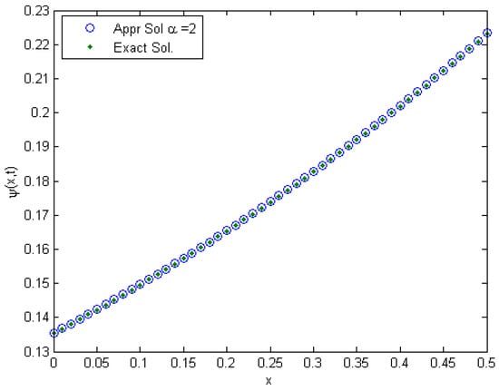
Figure 1. The Exact and Approximate Solutions of $\psi (x,t)$ for Example 1 for $\alpha =2$.

Table 1. Exact and Approximate Solution of $\psi (x,t)$ for Example 1.

t	Exact Solution	Approximate Sol	$\mathit{\psi }=|\mathit{\psi }-{\mathit{\psi }}_{10}|$
0.0	1.648721270700128	1.648721270700128	0.0
0.5	1.0	1.000000000040401	4.040101586 $e-11$
1.0	0.606530659712633	0.606530742852590	8.313995659 $e-8$
1.5	0.367879441171442	0.367886690723836	7.249552393 $e-6$
2.0	0.223130160148429	0.223303762933655	1.569783692 $e-4$

Figure 2 shows the exact solution and the approximate solution Equation (30) obtained by natural transform and Adomian decomposition method when $\alpha$ decreasing then the $\psi$ decreasing.

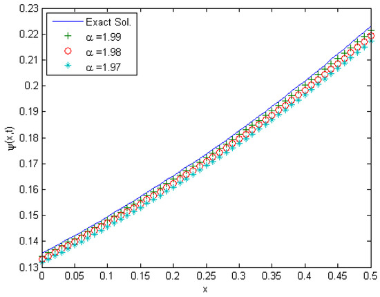
Figure 2. The Exact Solutions and Approximate Solutions of $\psi (x,t)$ for Example 1 for different value for $\alpha$.

Table 2 discuss the solution of Example 1 by choosing different values of $t=\{0,0.5,1,1.5,2\}$ and the values of $\psi (x,t)$ decreasing when t increasing for different values of $\alpha =1.99,1.98$ and $1.97.$

Table 2. Approximate Solution of $\psi (x,t)$ for Example 1.

t	$\mathit{\alpha }=1.99$	$\mathit{\alpha }=1.98$	$\mathit{\alpha }=1.97$
0.0	1.648721270700128	1.648721270700128	1.648721270700128
0.5	1.002243362235993	1.004498274095028	1.006764389796932
1.0	0.609569757949665	0.612585971492061	0.615579284214978
1.5	0.369222108754806	0.371788163947318	0.370522335669580
2.0	0.221291547575669	0.219269844467107	0.217240584657229

Figure 3 shows when setting $\alpha =2$ in the nth approximations and canceling noise terms yields the exact solution $\psi =|\psi -{\psi }_{10}|$ as $n\to \infty$. The analytical solution for the exact solution and the approximate solution Equation (42) obtained by natural transform and Adomian decomposition method. In addition, the exact solution is presented graphically in Figure 3.

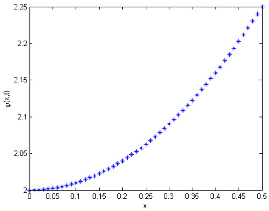
Figure 3. The exact solution of $\psi (x,t)$ for Example 2.

The exact and approximate solutions of Equation (52) are presented graphically in Figure 4, the approximate solution is given at $\alpha =1.99,1.98$ and $1.97$. The value of the solution satisfies Equation (52) see in Table 3 for the values $\alpha =1.99,1.98$ and $1.97$.

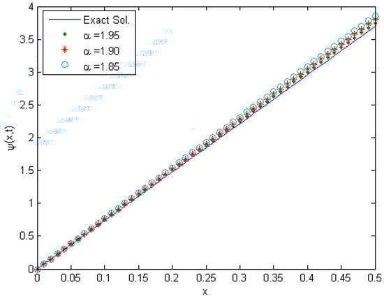
Figure 4. The approximate solutions of $\psi (x,t)$ for Example 3 for $\alpha =1.95$, $\alpha =1.90$, $\alpha =1.85$ and exact solution.

Table 3. Approximate solution of $\psi (x,t)$ for Example 3.

t	Exact Solution	$\mathit{\alpha }=1.95$	$\mathit{\alpha }=1.90$	$\mathit{\alpha }=1.85$
0.0	0.5	0.5	0.5	1.5
5.0	0.824360635350064	0.830817752645242	0.837755999175080	0.845202109327201
1.0	1.359140914229523	1.378259288907402	1.398076433466764	1.418592017094073
1.5	2.240844535169032	2.276244404149126	2.312171661003479	2.348587393416824
2.0	3.694528049465325	3.748855797997422	3.803171995755493	3.857406067787722

7. Conclusions

We have successfully applied the natural transform and Adomian decomposition method to obtain the approximate solutions of the fractional telegraph equation. The (NTDM) give us small error and high convergence. As seen in Table 1, Table 2 and Table 3, errors are very small, and sometimes deflate as shown in Table 3. These techniques lead us to say that the method is accurate and efficient according to theoretical analysis and examples 3 and 4 the exact solution and approximate solution of $\psi (x,t)$ are equal at $\alpha =2$ the absolute error equal zero.

References

- Hosseini, V.R.; Chen, W.; Avazzadeh, Z. Numerical solution of fractional telegraph equation by using radial basis functions. Eng. Anal. Bound. Elem. 2014, 38, 31–39. [Google Scholar] [CrossRef]
- Kumar, S. A new analytical modelling for fractional telegraph equation via Laplace transform. Appl. Math. Model. 2014, 38, 3154–3163. [Google Scholar] [CrossRef]
- Alawad, F.A.; Yousif, E.A.; Arbab, A.I. A new technique of Laplace variational iteration method for solving space-time fractional telegraph equations. Int. J. Differ. Equ. 2013, 2013, 256593. [Google Scholar] [CrossRef]
- Dhunde, R.R.; Waghmare, G. Double Laplace transform method for solving space and time fractional telegraph equations. Int. J. Math. Math. Sci. 2016, 2016, 1414595. [Google Scholar] [CrossRef]
- Biazar, J.; Shafiof, S. A simple algorithm for calculating Adomian polynomials. Int. J. Contemp. Math. Sci. 2007, 2, 975–982. [Google Scholar] [CrossRef]
- Garg, M.; Sharma, A. Solution of space-time fractional telegraph equation by Adomian decomposition method. J. Inequal. Spec. Funct. 2011, 2, 1–7. [Google Scholar]
- Kashuri, A.; Fundo, A.; Kreku, M. Mixture of a new integral transform and homotopy perturbation method for solving nonlinear partial differential equations. Adv. Pure Math. 2013, 3, 317. [Google Scholar] [CrossRef]
- Xu, H.; Liao, S.-J.; You, X.-C. Analysis of nonlinear fractional partial differential equations with the homotopy analysis method. Commun. Nonlinear Sci. Numer. Simul. 2009, 14, 1152–1156. [Google Scholar] [CrossRef]
- Saadatmandi, A.; Dehghan, M. Numerical solution of hyperbolic telegraph equation using the Chebyshev tau method. Numer. Methods Part. Differ. Equ. 2010, 26, 239–252. [Google Scholar] [CrossRef]
- Chen, J.; Liu, F.; Anh, V. Analytical solution for the time-fractional telegraph equation by the method of separating variables. J. Math. Anal. Appl. 2008, 338, 1364–1377. [Google Scholar] [CrossRef]
- Wazwaz, A.-M. Partial Differential Equations And Solitary Waves Theory; Springer Science & Business Media: Berlin/Heidelberg, Germany, 2010. [Google Scholar]
- Belgacem, F.B.M.; Silambarasan, R. Theory of natural transform. Math. Eng. Sci. Aerosp. J. 2012, 3, 99–124. [Google Scholar]
- Maitama, S. A hybrid natural transform homotopy perturbation method for solving fractional partial differential equations. Int. J. Differ. Equ. 2016, 2016, 9207869. [Google Scholar] [CrossRef]
- Shah, K.; Khalil, H.; Khan, R.A. Analytical solutions of fractional order diffusion equations by natural transform method. Iranian J. Sci. Technol. Trans. A Sci. 2016, 1–12. [Google Scholar] [CrossRef]
- Podlubny, I. Fractional Differential Equations: An Introduction to Fractional Derivatives, Fractional Differential Equations, to Methods of Their Solution and Some of Their Applications; Elsevier: Amsterdam, The Netherlands, 1998; Volume 198. [Google Scholar]
- El-Kalla, I. Convergence of the Adomian method applied to a class of nonlinear integral equations. Appl. Math. Lett. 2008, 21, 372–376. [Google Scholar] [CrossRef]
© 2019 by the authors. Licensee MDPI, Basel, Switzerland. This article is an open access article distributed under the terms and conditions of the Creative Commons Attribution (CC BY) license (http://creativecommons.org/licenses/by/4.0/).