Numerical Simulation of Partial Differential Equations via Local Meshless Method

Abstract

In this paper, numerical simulation of one, two and three dimensional partial differential equations (PDEs) are obtained by local meshless method using radial basis functions (RBFs). Both local and global meshless collocation procedures are used for spatial discretization, which convert the given PDEs into a system of ODEs. Multiquadric, Gaussian and inverse quadratic RBFs are used for spatial discretization. The obtained system of ODEs has been solved by different time integrators. The salient feature of the local meshless method (LMM) is that it does not require mesh in the problem domain and also far less sensitive to the variation of shape parameter as compared to the global meshless method (GMM). Both rectangular and non rectangular domains with uniform and scattered nodal points are considered. Accuracy, efficacy and ease implementation of the proposed method are shown via test problems.

1. Introduction

In present time, the use of PDEs are indispensable to many fields of modern physics, engineering and technology. Kortewege–de Vries–Burgers’ (KdVB) equation is of high importance for describing different mechanisms derived by Su and Gardner [1] and is given as follows

$$U_t+\alpha U{U}_x-\beta U_{xx}+\gamma U_{xxx}=0,$$

(1)

with initial and boundary conditions

$$U(x,0)=h_1(x)$$

(2)

$$\begin{array}{cc}\hfill U(a,t)& =h_2(t),U(b,t)=h_3(t),\hfill \end{array}$$

(3)

where $\alpha$, $\beta$ and $\gamma$ are arbitrary constants.

There are various physical applications of the KdVB equation such as dissipative effects in nonlinear plasma waves [2], shallow water wave description in viscous fluids [3], and propagation of waves in elastic tubes filled with a viscous fluid [4]. The KdVB equation has been solved by different numerical methods including meshless methods [5,6], the Chebyshev spectral collocation method [7], sinc-collocation method [8], and extended B-spline collocation method [9].

The coupled Drinfeld’s–Sokolov–Wilson equations is an important nonlinear PDE model which can be written as follows

$$\begin{array}{cc}\hfill U_t+3V{V}_x& =0,\hfill \\ \hfill V_t+2V_{xxx}+2U{V}_x+V{U}_x& =0.\hfill \end{array}$$

(4)

with initial and boundary conditions

$$\begin{array}{cc}\hfill U(x,0)& =f_1(x),V(x,0)=f_2(x),\hfill \\ \hfill U(a,t)& =f_3(t),U(b,t)=f_4(t),\hfill \\ \hfill V(a,t)& =f_5(t),V(b,t)=f_6(t).\hfill \end{array}$$

(5)

Different numerical methods such as the homotopy analysis method [10], meshless method of lines [11] and radial basis functions (RBFs) meshfree algorithm based on scattered data interpolation [12] can be found in the literature to obtain the solution of this model.

The two dimensional linear diffusion equation [13,14] is a vital model which is given as

$$U_t=\alpha (U_{xx}+U_{yy})\equiv \mathcal{L}U$$

(6)

$$\begin{array}{cc}\hfill U(x,y,0)& =I_1(x,y),\hfill \\ \hfill U(a,y,t)& =I_2(y,t),U(b,y,t)=I_3(y,t),\hfill \\ \hfill U(x,a,t)& =I_4(x,t),U(x,b,t)=I_5(x,t).\hfill \end{array}$$

(7)

where $\alpha$ is arbitrary constant.

Several authors have solved this model numerically including by the Meshless Local Petrov-Galerkin (MLPG) method [13], meshless local weak and strong forms [14] and MLPG method with improved weight function [15].

The two dimensional nonlinear regularized long wave (RLW) equation [16,17] along with initial and boundary conditions is given as

$$\begin{array}{c}\hfill \frac{\partial U}{\partial t}-\frac{\partial }{\partial t}\left(\frac{{\partial }^{2}U}{\partial x^2}+\frac{{\partial }^{2}U}{\partial y^2}\right)+\frac{\partial U}{\partial x}+\frac{\partial U}{\partial y}+U\frac{\partial U}{\partial x}+U\frac{\partial U}{\partial y}=0,(x,y)\in [a,b],t>0,\end{array}$$

(8)

$$\begin{array}{cc}\hfill U(x,y,0)& =g_1(x,y),\hfill \\ \hfill U(a,y,t)& =g_2(y,t),U(b,y,t)=g_3(y,t),\hfill \\ \hfill U(x,a,t)& =g_4(x,t),U(x,b,t)=g_5(x,t).\hfill \end{array}$$

(9)

The regularized long wave model equation described many physical phenomena [18]. Several methods exist for a numerical solution of this model equation such as finite-difference methods [19,20], interpolating the element-free Galerkin method [17], finite-element method [21], Fourier pseudo-spectral method [22] and cubic B-spline method [23]. Also, for the generalized RLW equation Petrov–Galerkin [24] and element-free Kp–Ritz [25] methods are used.

The three asset American-put option under the Black–Scholes model [26] is considered as a free boundary-value problem and can be written as [27]

$$\begin{array}{c}\hfill \frac{\partial U}{\partial t}=\frac{1}{2}{\sigma }_1^2{x}^2\frac{{\partial }^{2}U}{\partial x^2}+\frac{1}{2}{\sigma }_2^2{y}^2\frac{{\partial }^{2}U}{\partial y^2}+\frac{1}{2}{\sigma }_3^2{z}^2\frac{{\partial }^{2}U}{\partial z^2}+{\rho }_{12}{\sigma }_1{\sigma }_{2}xy\frac{{\partial }^{2}U}{\partial x\partial y}\\ \hfill +{\rho }_{13}{\sigma }_1{\sigma }_{3}xz\frac{{\partial }^{2}U}{\partial x\partial z}+{\rho }_{23}{\sigma }_2{\sigma }_{3}yz\frac{{\partial }^{2}U}{\partial y\partial z}+(r-D_1)x\frac{\partial U}{\partial x}\\ \hfill +(r-D_2)y\frac{\partial U}{\partial y}+(r-D_3)z\frac{\partial U}{\partial z}-rU,x,y,z\ge 0,t\in [0,T].\end{array}$$

(10)

The variables x, y, z are space variables showing prices of the underlying assets, r, $D_i$, ${\sigma }_i$, ${\rho }_{ij}$, T and U represent risk free interest rate, dividend paid by the i-th asset, volatility of the i-th underlying asset, correlation between the i-th and j-th assets, expiry time and value of the option respectively.

Using the penalty term approach [28,29], Equation (10) is converted into a fixed domain model in the following form

$$\begin{array}{c}\hfill \frac{\partial U}{\partial t}=\frac{1}{2}{\sigma }_1^2{x}^2\frac{{\partial }^{2}U}{\partial x^2}+\frac{1}{2}{\sigma }_2^2{y}^2\frac{{\partial }^{2}U}{\partial y^2}+\frac{1}{2}{\sigma }_3^2{z}^2\frac{{\partial }^{2}U}{\partial z^2}+{\rho }_{12}{\sigma }_1{\sigma }_{2}xy\frac{{\partial }^{2}U}{\partial x\partial y}\\ \hfill +{\rho }_{13}{\sigma }_1{\sigma }_{3}xz\frac{{\partial }^{2}U}{\partial x\partial z}+{\rho }_{23}{\sigma }_2{\sigma }_{3}yz\frac{{\partial }^{2}U}{\partial y\partial z}+(r-D_1)x\frac{\partial U}{\partial x}\\ \hfill +(r-D_2)y\frac{\partial U}{\partial y}+(r-D_3)z\frac{\partial U}{\partial z}-rU+\frac{\mu C}{U+\mu -q},x,y,z\ge 0,t\in [0,T],\end{array}$$

(11)

where $C\ge rE$, $q=E-({\alpha }_{1}x+{\alpha }_{2}y+{\alpha }_{3}z)$ and $0\le \mu \ll 1$.

The initial condition is given as

$$U(x,y,z,0)=E-({\alpha }_{1}x+{\alpha }_{2}y+{\alpha }_{3}z),x,y,z\ge 0.$$

The boundary conditions are given as

$$\begin{array}{cc}\hfill U(x,y,0,t)& =G_1(x,y),x,y\ge 0,t\in [0,T],\hfill \\ \hfill U(x,0,z,t)& =G_2(x,z),x,z\ge 0,t\in [0,T],\hfill \\ \hfill U(0,y,z,t)& =G_3(y,z),y,z\ge 0,t\in [0,T],\hfill \\ \hfill \underset{x\to \infty }{lim}U(x,y,z,t)& =0,y,z\ge 0,t\in [0,T],\hfill \\ \hfill \underset{y\to \infty }{lim}U(x,y,z,t)& =0,x,z\ge 0,t\in [0,T],\hfill \\ \hfill \underset{z\to \infty }{lim}U(x,y,z,t)& =0,x,y\ge 0,t\in [0,T].\hfill \end{array}$$

The functions $G_1$, $G_2$ and $G_3$ in the boundary are the solution of appropriate two asset American-put option problem. Various numerical methods such as [27,29,30,31,32] are utilized for solving American options.

Recently, the meshless methods have gotten broad attention for the solution of different kinds of PDEs arising in several different disciplines of engineering. The meshless character is one for the most important reasons for rising the demand of such types of methods. These methods eliminate the construction of difficult mesh and are easily extendible for interpolating multi-dimensional data as compared to other conventional methods. The numerical results of RBFs based algorithms have demonstrated that it is truly meshfree, accurate and east to implement. Some interesting models can be found in [30,33,34,35,36,37,38,39,40].

In the global meshless method (GMM), in case of shape parameter dependent RBFs, the selection of the optimum value of the shape parameter value c and dense ill-conditioned matrix are counted as a major deficiencies. To ward off the deficiencies in the GMM, the researchers [41,42] suggested local meshless methods. In the last few years, local meshless methods have been employed for the solution to complex PDE models (see [32,42,43]).

In the current work, the local meshless differential quadrature collocation method (LMM) is proposed for the numerical simulation of one dimensional Kortewege–de Vries–Burgers’, one dimensional coupled Drinfeld’s–Sokolov–Wilson, two dimensional linear diffusion and two dimensional regularized long wave equations. The LMM is an accurate and efficient numerical technique which requires two steps to approximate time-dependent PDEs. In the first step, space derivatives are approximated using RBFs which reduced the given PDE into a system of ODEs while in the second step, the system-obtained ODEs are solved by an appropriate ODE solver.

Contents of the rest of the paper are organized as follows; The suggested numerical method is highlighted in Section 2, time integration scheme is presented in Section 3, stability of the method is discussed in Section 4, implementation of the method to different test problems is presented in Section 5 and finally some conclusions are drawn in Section 6.

2. Implementation of Numerical Method

In this section a description of the LMM [33,43] is given for numerical solution of the PDE models given in Section 1. To pursue this, the derivatives of $U(x,t)$ at the center $x_i$ are approximated by the function values at a set of nodes in the neighbourhood of $\{x_{i_1},x_{i_2},x_{i_3},\dots ,x_{i_{n_i}}\}\subset \{x_1,x_2,\dots ,x_N\},n_i\ll N$,

$$U^{(m)}(x_i)\approx \sum _{k=1}^{n_i}{\lambda }_k^{(m)}U(x_{i_k}),i=1,2,\dots ,N.$$

(12)

Substituting RBF $\psi (\parallel x-x_l\parallel )$ into Equation (12) to find the corresponding coefficient ${\lambda }_k^{(m)}$

$${\psi }^{(m)}(\parallel x_i-x_l\parallel )=\sum _{k=1}^{n_i}{\lambda }_{i_k}^{(m)}\psi (\parallel x_{i_k}-x_l\parallel ),l=i_1,i_2,\dots ,i_{n_i}.$$

(13)

Equation (13) can be written as follows

$$\left[\begin{array}{c}{\psi }_{i_1}^{(m)}(x_i)\\ {\psi }_{i_2}^{(m)}(x_i)\\ ⋮\\ {\psi }_{i_{n_i}}^{(m)}(x_i)\end{array}\right]=\left[\begin{array}{cccc}{\psi }_{i_1}(x_{i_1})& {\psi }_{i_2}(x_{i_1})& \cdots & {\psi }_{i_{n_i}}(x_{i_1})\\ {\psi }_{i_1}(x_{i_2})& {\psi }_{i_2}(x_{i_2})& \cdots & {\psi }_{i_{n_i}}(x_{i_2})\\ ⋮& ⋮& \ddots & ⋮\\ {\psi }_{i_1}(x_{i_{n_i}})& {\psi }_{i_2}(x_{i_{n_i}})& \cdots & {\psi }_{i_{n_i}}(x_{i_{n_i}})\end{array}\right]\left[\begin{array}{c}{\lambda }_{i_1}^{(m)}\\ {\lambda }_{i_2}^{(m)}\\ ⋮\\ {\lambda }_{i_{n_i}}^{(m)}\end{array}\right],$$

(14)

where

$${\psi }_l(x_k)=\psi (\parallel x_k-x_l\parallel ),l=i_1,i_2,\dots ,i_{n_i},$$

for each $k=i_1,i_2,\dots ,i_{n_i}$.

Matrix notation of Equation (14) is

$${\mathit{\psi }}_{n_i}^{(m)}={\mathbf{A}}_{n_i}{\mathit{\lambda }}_{n_i}^{(m)},$$

(15)

where

$${\mathit{\psi }}_{n_i}^{(m)}={\left[\begin{array}{cccc}{\psi }_{i_1}^{(m)}(x_i)& {\psi }_{i_2}^{(m)}(x_i)& \cdots & {\psi }_{i_{n_i}}^{(m)}(x_i)\end{array}\right]}^T,$$

$${\mathbf{A}}_{n_i}=\left[\begin{array}{cccc}{\psi }_{i_1}(x_{i_1})& {\psi }_{i_2}(x_{i_1})& \cdots & {\psi }_{i_{n_i}}(x_{i_1})\\ {\psi }_{i_1}(x_{i_2})& {\psi }_{i_2}(x_{i_2})& \cdots & {\psi }_{i_{n_i}}(x_{i_2})\\ ⋮& ⋮& \ddots & ⋮\\ {\psi }_{i_1}(x_{i_{n_i}})& {\psi }_{i_2}(x_{i_{n_i}})& \cdots & {\psi }_{i_{n_i}}(x_{i_{n_i}})\end{array}\right],$$

$${\mathit{\lambda }}_{n_i}^{(m)}={\left[\begin{array}{cccc}{\lambda }_{i_1}^{(m)}& {\lambda }_{i_2}^{(m)}& \cdots & {\lambda }_{i_{n_i}}^{(m)}\end{array}\right]}^T.$$

From Equation (15), we obtain

$${\mathit{\lambda }}_{n_i}^{(m)}={\mathbf{A}}_{n_i}^{-1}{\mathit{\psi }}_{n_i}^{(m)}.$$

(16)

From Equation (12) and Equation (16), we get

$$\begin{array}{c}\hfill U^{(m)}(x_i)={({\mathit{\lambda }}_{n_i}^{(m)})}^T{\mathbf{u}}_{n_i},\end{array}$$

where

$${\mathbf{U}}_{n_i}={\left[U(x_{i_1}),U(x_{i_2}),\dots ,U(x_{i_{n_i}})\right]}^T.$$

Local Meshless Method for KdVB Equation

Using the LMM to Equation (1) in space, we get

$$\begin{array}{c}\hfill \frac{d{U}_i}{dt}=-\alpha U_i{({\mathit{\lambda }}_{n_i}^{(1)})}^T{\mathbf{U}}_{n_i}+\beta {({\mathit{\lambda }}_{n_i}^{(2)})}^T{\mathbf{U}}_{n_i}-\gamma {({\mathit{\lambda }}_{n_i}^{(3)})}^T{\mathbf{U}}_{n_i},i=2,3,\dots ,N-1.\end{array}$$

(17)

The semi-discretized model Equation (17) with corresponding boundary conditions Equation (3) is given as follows

$$\frac{d\mathbb{U}}{dt}=-\alpha \mathbb{U}\ast ({\Lambda }^{(1)}\mathbb{U})+\beta ({\Lambda }^{(2)}\mathbb{U})-\gamma ({\Lambda }^{(3)}\mathbb{U}),$$

(18)

where the symbol * represents element-wise multiplication of two vectors.

$$\begin{array}{cc}\hfill \mathbb{U}& ={[U_1,U_2,U_3,\dots ,U_N]}^T,\hfill \\ \hfill {\Lambda }_{N\times N}^{(1)}& =\left[m_{ik}\right]=\left[{\mathit{\lambda }}_k^{(1)}\right],k=i_1,i_2,\dots ,i_{n_j},i=2,3,\dots ,N-1,\hfill \\ \hfill {\Lambda }_{N\times N}^{(2)}& =\left[m_{ik}\right]=\left[{\mathit{\lambda }}_k^{(2)}\right],k=i_1,i_2,\dots ,i_{n_j},i=2,3,\dots ,N-1,\hfill \\ \hfill {\Lambda }_{N\times N}^{(3)}& =\left[m_{ik}\right]=\left[{\mathit{\lambda }}_k^{(3)}\right],k=i_1,i_2,\dots ,i_{n_j},i=2,3,\dots ,N-1.\hfill \end{array}$$

(19)

The corresponding initial condition Equation (2) is given as

$$\mathbb{U}(t_0)={[U_0(x_1),U_0(x_2),\dots ,U_0(x_N)]}^T.$$

(20)

Up to now, the spatial derivatives are approximated by RBFs and the given PDE is reduced to a system of ODEs. Next, any ODE solver is needed to solve this system of ODEs.

3. Time Discretization

In this paper, three integration techniques, explicit Euler method (EEM), implicit method (IM) and the Crank–Nicolson method (CNM), are used to solve PDE models given in Section 1 and its explanation is given as:

A $\theta$-Weighted Technique for 2D Diffusion Equation

Applying $\theta$-weighted technique to approximate Equation (6) in time, we have

$$\begin{array}{cc}\hfill \frac{\partial U}{\partial t}& =\alpha (U_{xx}+U_{yy})\equiv \mathcal{L}U,\hfill \end{array}$$

as

$$\frac{U^{(n+1)}-U^{(n)}}{dt}=\theta \mathcal{L}{U}^{(n+1)}+(1-\theta )\mathcal{L}{U}^{(n)},$$

we get

$$U^{(n+1)}={(I-dt\theta \mathcal{L})}^{-1}\left[(I+dt(1-\theta )\mathcal{L})U^{(n)}\right].$$

(21)

After applying the LMM (discussed in Section 2), Equation (21) leads to

$$U^{(n+1)}={(I-dt\theta L)}^{-1}\left[(I+dt(1-\theta )L)U^{(n)}\right],$$

(22)

where L is the weight matrix of the differential operator $\mathcal{L}$ and I is an identity matrix. Equation (22) reduces to EEM, CNM and IM for $\theta =0$, $\theta =0.5$ and $\theta =1$ respectively.

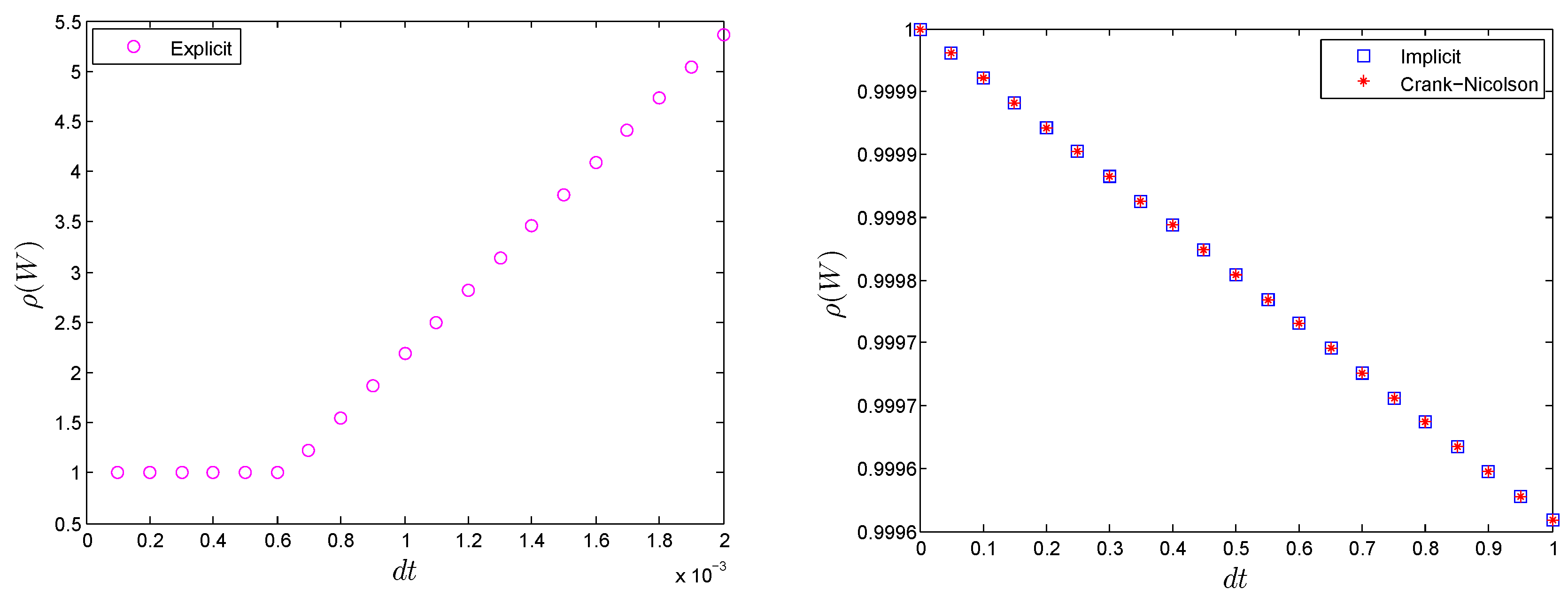
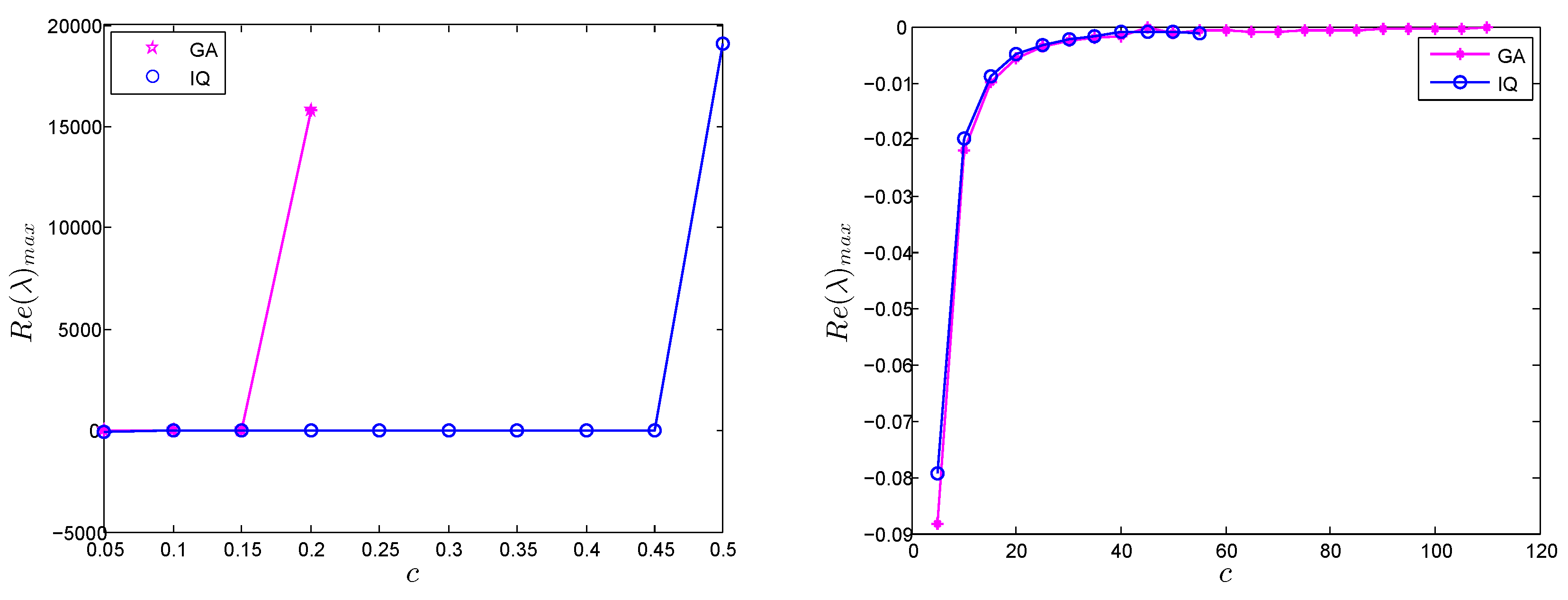
4. Stability Analysis

In this section, we used the matrix method for the stability of the local and global meshless methods as reported in [32,43]. $E^{(n)}$ is n-th time level error given by $E^{(n)}={\widehat{U}}^{(n)}-U^{(n)}$, which is introduced in Equation (22), where ${\widehat{U}}^{(n)}$ is the exact solution and $U^{(n)}$ is the approximate solution obtained by the LMM. The error $E^{(n+1)}$ can be expressed as

$$E^{(n+1)}=W{E}^{(n)},$$

(23)

where $W={[I-\theta dtL]}^{-1}[I+(1-\theta )dtL]$ is the amplification matrix. $\rho (W)$ denotes the spectral radius of W so the sufficient condition for numerical stability is $\rho (W)\le 1$, which leads to the following formula

$$\left|\frac{1+(1-\theta )dt\lambda }{1-\theta dt\lambda }\right|\le 1,$$

(24)

where $\lambda$ is eigenvalue of the matrix L.

The inequality Equation (24) reduces to

IM for $\theta =1$,

$$\left|\frac{1}{1-dt\lambda }\right|\le 1.$$

(25)

CNM for $\theta =0.5$,

$$\left|\frac{1+0.5dt\lambda }{1-0.5dt\lambda }\right|\le 1.$$

(26)

EEM for $\theta =0$,

$$\left|\frac{1+dt\lambda }{1}\right|\le 1,$$

(27)

that is,

$$dt\le \frac{-2}{\lambda }and\lambda \le 0,$$

(28)

In the case of complex eigenvalue $\lambda =c+id$, where c, d are any real numbers, the inequalities Equations (25)–(27) take the following form

For $FIM$

$$\left|\frac{1}{1-dt(c+id)}\right|\le 1,$$

implies

$$\frac{1}{\sqrt{1+d{t}^2{c}^2+d{t}^2{d}^2-2dtc}}\le 1.$$

(29)

For CNM

$$\left|\frac{1+0.5dt(c+id)}{1-0.5dt(c+id)}\right|\le 1,$$

implies

$$\sqrt{\frac{1+0.25d{t}^2{c}^2+0.25d{t}^2{d}^2+dtc}{1+0.25d{t}^2{c}^2+0.25d{t}^2{d}^2-dtc}}\le 1.$$

(30)

Similarly, for FEDF

$$\left|\frac{1+dt(c+id)}{1}\right|\le 1,$$

implies

$$dt\le \frac{-2c}{c^2+d^2},$$

(31)

provided $Re(\lambda )\le 0$ in all the inequalities in Equations (25)–(31).

The inequalities in Equations (25)–(27) guarantee unconditional stability in case of implicit and Crank–Nicolson schemes. Conditional stability in case of explicit scheme is also shown in Figure 1. The stability of meshless methods also depends on the value of the shape parameter c. The GMM is sensitive to the value of c in comparison to the LMM and the system gets ill-conditioned quickly by varying c. We investigated this dependence numerically in Figure 2. It can be seen from the figure that the LMM satisfies the stability condition for a wide range of this parameter.

Figure 3 shows sparsity pattern of the LMM corresponding to local sub-domain three in the 1D case and stencil size five in the 2D case. In comparison, the coefficient matrix of the global meshless method is dense. From the comparison of the coefficient matrices of both the local and the global meshless methods, it is clear that local meshless method produces sparse banded matrices which can be efficiently solved by sparse matrix solvers. In case of the global meshless method, the coefficient matrix is fully dense and often ill-conditioned. In such a scenario, a traditional solver, like Gauss elimination method, produces inaccurate results. Special procedure like truncated singular value decomposition (TSVD )is a more appropriate choice in such cases.

5. Numerical Analysis

The performance of the LMM is demonstrated against some problems in this section. The proposed scheme works for any radial basis functions but in the present work; multiquadric (MQ), Gaussian (GA), and inverse quadratic (IQ) RBFs are taken into account for spatial discretization. The proposed LMM is capable of approximating the solution on both the uniform and scattered nodal points. The size of a local sub-domain in one, two and three dimensional cases were taken to be three, five and seven, respectively. Computational efficiency and less sensitivity to the value of the shape parameter c were the major gains of the LMM, as GMM was found very sensitive to the value of shape parameter c. All the computations were performed using MATLAB (R2012a) on a Dell PC Laptop (Windows 7, 64 Bit) with an Intel (R) Core(TM)i5-240M CPU 2.50 GHz 2.5 GHs 4 GB RAM.

Accuracy of the LMM were measured via $L_{abs}$, $L_{\infty }$ and $L_R$ error norms which are given as follows

$$\begin{array}{cc}\hfill L_{abs}& =|\widehat{U}(i)-U(i)|,i=1,2,\dots ,N^n.\hfill \\ \hfill L_{\infty }& =\max \left(L_{abs}\right),\hfill \\ \hfill L_R& ={\left[\frac{1}{{\sum }_{i=1}^N{(\widehat{U}(i))}^2}\sum _{i=1}^N{L_{abs}}^2\right]}^{\frac{1}{2}},\hfill \end{array}$$

(32)

where $\widehat{U}$, U denote exact and approximate solutions respectively.

Problem 1.

The 1D KdVB Equation (1) with $\alpha =1$, having the following exact solution [5]

$$U(x,t)=-\frac{6{\beta }^2}{25\gamma }\left(1+tanh(\xi )+\frac{1}{2}sec{h}^2(\xi )\right),x\in [a,b],t\ge 0$$

(33)

where

$$\xi =\frac{\beta }{10\gamma }\left(x+\frac{6{\beta }^2}{25\gamma }t\right).$$

(34)

In

Table 1. Comparison of the numerical solution of the Kortewege–de Vries–Burgers’ (KdVB) equation for Problem 1.

t	${\mathit{L}}_{\mathbf{\infty }}$ LMM	${\mathit{L}}_2$ LMM	${\mathit{L}}_{\mathbf{\infty }}$ [5]	${\mathit{L}}_2$ [5]
	$\beta =0.004$
1	5.5555 × 10${}^{-12}$	2.8402 × 10${}^{-10}$	6.822 × 10${}^{-0}$	8.845 × 10${}^{-9}$
2	1.1110 × 10${}^{-11}$	5.6792 × 10${}^{-10}$	1.150 × 10${}^{-8}$	1.652 × 10${}^{-8}$
3	1.6661 × 10${}^{-11}$	8.5171 × 10${}^{-10}$	1.485 × 10${}^{-8}$	2.338 × 10${}^{-8}$
10	5.5441 × 10${}^{-11}$	2.8353 × 10${}^{-9}$	2.479 × 10${}^{-8}$	6.046 × 10${}^{-8}$
	$\beta =0.04$
1	8.4705 × 10${}^{-8}$	1.5103 × 10${}^{-6}$	2.936 × 10${}^{-6}$	3.727 × 10${}^{-7}$
2	1.6937 × 10${}^{-7}$	3.0211 × 10${}^{-6}$	4.204 × 10${}^{-6}$	2.207 × 10${}^{-8}$
3	2.5400 × 10${}^{-7}$	4.5322 × 10${}^{-6}$	4.126 × 10${}^{-6}$	1.928 × 10${}^{-6}$
10	8.4535 × 10${}^{-7}$	1.5111 × 10${}^{-5}$	5.800 × 10${}^{-6}$	1.297 × 10${}^{-5}$
	$\beta =0.1$
1	7.7105 × 10${}^{-6}$	1.1800 × 10${}^{-5}$	1.540 × 10${}^{-5}$	1.004 × 10${}^{-5}$
2	1.5374 × 10${}^{-5}$	2.3912 × 10${}^{-5}$	3.076 × 10${}^{-5}$	1.732 × 10${}^{-5}$
3	2.2987 × 10${}^{-5}$	3.6284 × 10${}^{-5}$	4.604 × 10${}^{-5}$	2.874 × 10${}^{-5}$
10	7.4772 × 10${}^{-5}$	1.2861 × 10${}^{-4}$	1.498 × 10${}^{-4}$	1.342 × 10${}^{-4}$

, numerical results of the LMM for Problem 1 using different values of $\beta$ and time t over the space interval $[-20,20]$ are shown. We took $\alpha =1$, $\gamma =0.1$, $dt=0.001$, $N=81$ and MQ RBF with $c=100$. Better results of the LMM as compared to the result given in [5] were clear from the table. In Figure 4 and Figure 5 solution profiles are shown for different values of $\beta$.

The numerical solution of the KdVB equation for different time t in Problem 1 with time step length $dt=0.02$, $\alpha =2$, $\beta =0.005$, $\gamma =0.1$, $N=101$, spatial domain $[-100,100]$ are shown in

Table 2. Comparison of numerical solution of the KdVB equation for Problem 1.

t	${\mathit{L}}_{\mathbf{\infty }}$	${\mathit{L}}_2$	CPU Time	${\mathit{L}}_{\mathbf{\infty }}$	${\mathit{L}}_2$
	LMM	LMM	LMM	[8]	[8]
1	2.8316 × 10${}^{-10}$	3.1032 × 10${}^{-8}$	0.26	2.06127 × 10${}^{-6}$	4.62479 × 10${}^{-6}$
3	8.4947 × 10${}^{-10}$	9.3095 × 10${}^{-8}$	0.72	1.14705 × 10${}^{-6}$	9.14997 × 10${}^{-7}$
5	1.4158 × 10${}^{-9}$	1.5515 × 10${}^{-7}$	1.15	1.28565 × 10${}^{-6}$	1.21327 × 10${}^{-6}$
7	1.9821 × 10${}^{-9}$	2.1721 × 10${}^{-7}$	1.63	1.51656 × 10${}^{-6}$	1.45490 × 10${}^{-6}$
9	2.5484 × 10${}^{-9}$	2.7927 × 10${}^{-7}$	2.18	1.67755 × 10${}^{-6}$	1.66392 × 10${}^{-6}$

. It is clear from the table that the LMM was a more accurate than the method in reported in [8].

Problem 2.

The analytical solution [44] of the 1D coupled Drinfeld’s–Sokolov–Wilson system (4) is given as

$$\begin{array}{cc}\hfill U(x,t)& =\frac{(\alpha -4k)}{2}+3k^{2}sec{h}^2\left(k(x-\alpha t)\right),\hfill \\ \hfill V(x,t)& =2k\sqrt{\frac{\alpha }{2}}sech\left(k(x-\alpha t)\right).\hfill \end{array}$$

(35)

The numerical simulations for Problem 2 are reported in

Table 3. Comparison of the $L_{\infty }$ error norm of $U(x,t)$ for Problem 2.

	${\mathit{L}}_{\mathbf{\infty }}$
	x = 0.1		x = 0.3		x = 0.5
t	LMM	[11]	LMM	[11]	LMM	[11]
0.1	4.44 × 10${}^{-16}$	4.5230 × 10${}^{-13}$	5.55 × 10${}^{-17}$	1.3291 × 10${}^{-12}$	6.10 × 10${}^{-16}$	6.6992 × 10${}^{-12}$
0.2	2.16 × 10${}^{-15}$	1.3524 × 10${}^{-12}$	1.22 × 10${}^{-15}$	1.3696 × 10${}^{-12}$	1.11 × 10${}^{-16}$	2.1989 × 10${}^{-12}$
0.3	5.21 × 10${}^{-15}$	2.2525 × 10${}^{-12}$	3.83 × 10${}^{-15}$	4.0690 × 10${}^{-12}$	2.16 × 10${}^{-15}$	2.3009 × 10${}^{-12}$
0.4	9.60 × 10${}^{-15}$	3.1523 × 10${}^{-12}$	7.71 × 10${}^{-15}$	6.7682 × 10${}^{-12}$	5.55 × 10${}^{-15}$	6.8008 × 10${}^{-12}$
0.5	1.53 × 10${}^{-14}$	4.0521 × 10${}^{-12}$	1.29 × 10${}^{-14}$	9.4666 × 10${}^{-12}$	1.03 × 10${}^{-14}$	1.1300 × 10${}^{-11}$

and

Table 4. Comparison of the $L_{\infty }$ error norm of $V(x,t)$ for Problem 2.

	${\mathit{L}}_{\mathbf{\infty }}$
	x = 0.1		x = 0.3		x = 0.5
t	LMM	[11]	LMM	[11]	LMM	[11]
0.1	7.81 × 10${}^{-12}$	2.2379 × 10${}^{-11}$	2.30 × 10${}^{-11}$	6.9696 × 10${}^{-11}$	3.82 × 10${}^{-11}$	1.2050 × 10${}^{-10}$
0.2	1.60 × 10${}^{-11}$	4.4328 × 10${}^{-11}$	4.64 × 10${}^{-11}$	1.3552 × 10${}^{-10}$	7.69 × 10${}^{-11}$	2.3025 × 10${}^{-10}$
0.3	2.46 × 10${}^{-11}$	6.6276 × 10${}^{-11}$	7.03 × 10${}^{-11}$	2.0134 × 10${}^{-10}$	1.15 × 10${}^{-10}$	3.3999 × 10${}^{-10}$
0.4	3.37 × 10${}^{-11}$	8.8225 × 10${}^{-11}$	9.46 × 10${}^{-11}$	2.6716 × 10${}^{-10}$	1.55 × 10${}^{-10}$	4.4973 × 10${}^{-10}$
0.5	4.31 × 10${}^{-11}$	1.1017 × 10${}^{-10}$	1.19 × 10${}^{-10}$	3.3298 × 10${}^{-10}$	1.95 × 10${}^{-10}$	5.5947 × 10${}^{-10}$

of the coupled Drinfeld’s–Sokolov–Wilson system Equation (4) on the spatial domain $[-4,4]$ from $t=0.1$ to $t=0.5$ with $N=81$ and $dt=0.0001$. Table 3 and Table 4 show the $L_{\infty }$ error norm of the LMM along with the comparison of the meshless method of lines based on RBFs [11] for $\alpha =1$, $k=0.001$ and $\alpha =0.0001$, $k=0.01$ respectively. One can guarantee from this comparison that the results of the LMM are more effective.

Table 5. Numerical solution for a wide range of the shape parameter value c for $\alpha =0.0001$ and $k=0.01$ for Problem 2.

c	U	V	c	U	V
0.001	1.4629 × 10${}^{-12}$	3.0635 × 10${}^{-9}$	40	6.0559 × 10${}^{-13}$	1.2333 × 10${}^{-9}$
0.01	1.1800 × 10${}^{-11}$	2.0888 × 10${}^{-7}$	80	5.6560 × 10${}^{-13}$	1.1480 × 10${}^{-9}$
0.1	1.1655 × 10${}^{-11}$	2.2179 × 10${}^{-7}$	160	5.5559 × 10${}^{-13}$	1.1268 × 10${}^{-9}$
1	1.1747 × 10${}^{-11}$	2.0555 × 10${}^{-7}$	320	5.5265 × 10${}^{-13}$	1.1216 × 10${}^{-9}$
5	3.8443e × 10${}^{-12}$	1.0146 × 10${}^{-8}$	640	5.9097 × 10${}^{-13}$	1.1239 × 10${}^{-9}$
10	1.4029 × 10${}^{-12}$	3.0469 × 10${}^{-9}$	1000	9.0130 × 10${}^{-13}$	1.1524 × 10${}^{-9}$
20	7.6552 × 10${}^{-13}$	1.5794 × 10${}^{-9}$	1200	6.1639 × 10${}^{-13}$	1.1081 × 10${}^{-9}$

and

Table 6. Numerical solution for the range of the shape parameter value c for $\alpha =0.0001$ and $k=0.01$ for Problem 2.

$\mathit{c}$	0.001	0.01	0.1	0.2	0.3
U	2.8405 × 10${}^{-10}$	3.4306 × 10${}^{-9}$	3.5230 × 10${}^{-10}$	1.4130 × 10${}^{-10}$	⋯
V	5.2746 × 10${}^{-7}$	6.5458 × 10${}^{-6}$	9.1756 × 10${}^{-7}$	3.5451 × 10${}^{-}7$	⋯

show numerical results of the LMM and the GMM of the coupled Drinfeld’s–Sokolov–Wilson system Equation (4) for $N=81$, $dt=0.0001$, $t=0.5$, and different values of c. The accuracy of the global RBF methods is heavily dependent on c and this is evident from Table 6 as well. From the comparison shown in Table 5 and Table 6, one can observe that the value of c was not an issue in the LMM as compared to the GMM.

Problem 3.

The exact solution [13] of the 2D linear diffusion Equation (6) with $\alpha =1$ is given as

$$U(x,y,t)=exp(x+y+2t),(x,y)\in {[0,1]}^2,t\ge 0.$$

(36)

The proposed LMM is employed on the test Problem Equation (3) and the results are shown in Figure 6 by having a time step length of $dt=0.0001$, the shape parameter value of MQ RBF $c=100$ and $N=20\times 20$, at different times, up to $t=1$. Furthermore, the results obtained by the LMM (Crank–Nicolson) have been compared in order to verify the accuracy of the LMM with the results reported in [13,14], which confirm the validity of the presented method.

The numerical results of the 2D linear diffusion Equation (6) on non rectangular domains are shown in Figure 7, Figure 8, Figure 9, Figure 10 and Figure 11 for Problem 3 using GA RBF. The numerical results shown in Figure 7, Figure 8, Figure 9, Figure 10 and Figure 11 are performed with $dt=0.0001$, $t=1$ and $\alpha =1$. These figures show the efficiency of the LMM in non rectangular domains in term of absolute error $L_{abs}$ norm for Problem 3.

Problem 4.

Finally, consider a two-dimensional nonlinear RLW Equation (8) with the following exact solution

$$U(x,y,t)=\frac{q}{2}sec{h}^2\left(\frac{\sqrt{q}}{2p}(x+y-vt-x_0-y_0)\right),(x,y)\in {[-80,100]}^2,t\ge 0,$$

(37)

where $q=\frac{6(v-2)}{2}$ and $p=\sqrt{6v}$.

Table 7. Numerical results in term of $L_{\infty }$ error norm for Problem 4.

t	1	5	10	15	20
$L_{\infty }$	6.8814 × 10${}^{-4}$	3.4458 × 10${}^{-3}$	7.0255 × 10${}^{-3}$	1.2374 × 10${}^{-2}$	2.0904 × 10${}^{-2}$
CPU time (in s)	2.54	2.59	2.71	2.85	2.88

shows numerical results in terms of $L_{\infty }$ error norm and CPU time for Problem 4 with $v=2.06$, $N=50$, $dt=0.5$, $[-80,100]$ and up to time $t=20$. From this table, it is evident that the proposed LMM is accurate and efficient.

Numerical results at $t=1$ and $t=10$ with $v=2.06$, $N=50$, $dt=0.5$, $[-80,100]$ for Problem 4 are shown in Figure 12.

In Figure 13 the $L_{abs}$ error are shown at $t=10$.

Eliminating the need of meshing and approximating the solution using uniform or scattered points in rectangular as well non-rectangular domains is one of the salient feature of the LMM. Numerical results of the RLW equation on non-rectangular domains are shown in Figure 14 and Figure 15.

Figure 16 (left) is evidence to the fact that, in case of LMM, the sensitivity to the shape parameter value is no longer a major problem. In Figure 16 (right) the condition number $\kappa$ is also shown.

Comparison of CPU time of the LMM and the GMM are shown in Figure 17 by taking $dt=0.01$ and $t=10$. It is clear from this figure that LMM was more efficient then GMM.

Problem 5.

Three asset American-put option with parameters $r=0.1$, ${\sigma }_1=0.2$, ${\sigma }_2=0.3$, ${\sigma }_3=0.2$, ${\alpha }_1=0.3$, ${\alpha }_2=0.3$, ${\alpha }_3=0.4$, $D_1=0.05$, $D_2=0.01$, $D_3=0.01$, ${\rho }_{12}={\rho }_{13}={\rho }_{23}=0.5$, $\mu =0.01$, $E=1$, $T=1$ years, $dt=0.001$ and spatial domain ${[0,4]}^3$.

Table 8. CPU time and option value for Problem 5.

N	P(1,1,1)	P(1.1,1.1,1.1)	CPU Time
$8\times 8\times 8$	0.051746	0.0278333	7.6
$12\times 12\times 12$	0.055708	0.021232	32.7
$16\times 16\times 16$	0.058240	0.020440	128.9
$20\times 20\times 20$	0.059639	0.020797	554.9

shows the numerical solution and CPU time (in s) of three asset American-put option for Problem 5 using LMM. The time step was $dt=0.001$ and we had a fixed value of shape parameter $c=10$, whereas

Table 9. $L_{abs}$ error norm for Problem 5.

N	${\mathit{L}}_{\mathit{abs}}$ at P(1,1,1)	${\mathit{L}}_{\mathit{abs}}$ at P(1.1,1.1,1.1)
$4\times 4\times 4$	9.7425 × 10${}^{-3}$	2.0440 × 10${}^{-2}$
$8\times 8\times 8$	6.4939 × 10${}^{-3}$	7.3929 × 10${}^{-3}$

shows the $L_{abs}$ error at P$(1,1,1)$ and P$(1.1,1.1,1.1)$. The numerical solution of the American-put option are shown in Figure 18.

6. Conclusions

In the present work, the local meshless method based on radial basis functions is applied to one, two and three dimensional PDEs. To check the accuracy and efficacy of the proposed scheme on both rectangular and non-rectangular domains, different problems have been considered. Results of the local meshless method are compared with exact/approximate solutions available in the existent literature. The local meshless method has been found to be a flexible interpolation method as it removes sensitivity of the shape parameter and produces the coefficient matrix well-conditioned.

References

1. Su, C.H.; Gardner, C.S. Derivation of the Kortewege-de Vries and Burgers’ equation. J. Math. Phys. 1969, 10, 536–539. [Google Scholar] [CrossRef]
2. Grad, H.; Hu, P.N. Unified shock profile in a plasma. J. Mech. Phys. Solids 1967, 10, 2596–2601. [Google Scholar] [CrossRef]
3. Jonson, R.S. Shallow water waves in a viscous fluid-the undular bore. Phys. Fluids 1972, 15, 1993–1999. [Google Scholar] [CrossRef]
4. Jonson, R.S. A nonlinear equation incorporating damping and dispersion. J. Math. Fluid Mech. 1970, 42, 49–60. [Google Scholar] [CrossRef]
5. Sirajul, H.; Uddin, M. A mesh-free method for the numerical solution of the KdV-Burgers’ equation. Appl. Math. Model. 2009, 33, 3442–3449. [Google Scholar]
6. Ali, A.; Mukhtar, S.; Hussain, I. A numerical meshless technique for the solution of some Burgers’ type equations. World Appl. Sci. J. 2011, 12, 1792–1798. [Google Scholar]
7. Khater, A.H.; Temsah, R.S.; Hassan, M.M. Journal of computational and applied mathematics. J. Comput. Appl. Math. 2008, 222, 333–350. [Google Scholar] [CrossRef]
8. Sajjadian, M. Numerical solutions of Korteweg-de Vries and Korteweg-de Vries-Burgers’ equations using computer programming. Int. J. Nonlinear Sci. 2013, 15, 69–79. [Google Scholar]
9. Hepson, O.E.; Korkmaz, A.; Dag, I. Extended B-spline collocation method for KdV-Burgers’ equation. arXiv, 2017; arXiv:1701.02893. [Google Scholar]
10. Arora, R.; Kumar, A. Solution of the coupled Drinfeld’s-Sokolov-Wilson (DSW) system by homotopy analysis method. Adv. Sci. Eng. Med. 2013, 5, 1105–1111. [Google Scholar] [CrossRef]
11. Sirajul, H.; Hassan, N.; Tirmizi, S.I.A.; Usman, M. A Meshless Method of Lines for the Numerical Solution of Coupled Drinfeld’s-Sokolov-Wilson System; Elsevier: Amsterdam, The Netherlands, 2010. [Google Scholar]
12. Uddin, M.; Haq, S. Application of a numerical method using radial basis functions to nonlinear partial differential equations. Selcuk J. Appl. Math. 2011, 12, 77–93. [Google Scholar]
13. Abbasbandy, S.; Shirzadi, A. MLPG method for two-dimensional diffusion equation with Neumann’s and non-classical boundary conditions. Appl. Numer. Math. 2011, 61, 170–180. [Google Scholar] [CrossRef]
14. Abbasbandy, S.; Ghehsareh, H.R.; Alhuthali, M.S.; Alsulami, H.H. Comparison of meshless local weak and strong forms based on particular solutions for a non-classical 2-D diffusion model. Eng. Anal. Bound. Elem. 2014, 39, 121–128. [Google Scholar] [CrossRef]
15. Techapirom, T.; Luadsong, A. The MLPG with improved weight function for two-dimensional heat equation with non-local boundary condition. J. King Saud Univ. Sci. 2013, 25, 341–348. [Google Scholar] [CrossRef] [Green Version]
16. Dehghan, M.; Salehi, R. The solitary wave solution of the two-dimensional regularized long-wave equation in fluids and plasmas. Comput. Phys. Commun. 2011, 182, 2540–2549. [Google Scholar] [CrossRef]
17. Dehghana, M.; Abbaszadeha, M.; Mohebbib, A. The use of interpolating element-free Galerkin technique for solving 2D generalized Benjamin-Bona-Mahony-Burgers and regularized long-wave equations on non-rectangular domains with error estimate. J. Comput. Appl. Math. 2015, 286, 211–231. [Google Scholar] [CrossRef]
18. Abdulloev, K.O.; Bogolubsky, I.L.; Makhankov, V.G. One more example of inelastic soliton interaction. Phys. Lett. 1976, 56, 427–428. [Google Scholar] [CrossRef]
19. Bona, J.L.; Bryant, P.J. A mathematical model for long waves generated by wave makers in nonlinear dispersive systems. Proc. Camb. Philos. Soc. 1973, 73, 391–405. [Google Scholar] [CrossRef]
20. Bhardwaj, D.; Shankar, R. A computational method for regularized long wave equation. Comput. Math. Appl. 2000, 40, 1397–1404. [Google Scholar] [CrossRef] [Green Version]
21. Esen, A.; Kutluay, S. Application of a lumped Galerkin method to the regularized long wave equation. Appl. Math. Comput. 2006, 174, 833–845. [Google Scholar] [CrossRef]
22. Gou, B.Y.; Cao, W.M. The Fourier pseudospectral method with a restrain operator for the RLW equation. Comput. Math. Appl. 1988, 74, 110–126. [Google Scholar]
23. Raslan, K.R. A computational method for the regularized long wave equation. Appl. Math. Comput. 2005, 167, 1101–1118. [Google Scholar] [CrossRef]
24. Roshan, T. A Petrov-Galerkin method for solving the generalized regularized long wave (GRLW) equation. Comput. Math. Appl. 2012, 63, 943–956. [Google Scholar] [CrossRef]
25. Guo, P.F.; Zhang, L.W.; Liew, K.M. Numerical analysis of generalized regularized long wave equation using the element-free kp-Ritz method. Appl. Math. 2014, 240, 91–101. [Google Scholar] [CrossRef]
26. Fischer, B.; Scholes, M. The pricing of options and corporate liabilities. J. Polit. Econ. 1973, 81, 637–654. [Google Scholar]
27. Martín-Vaquero, J.; Khaliq, A.Q.M.; Kleefeld, B. Stabilized explicit Runge-Kutta methods for multi-asset American options. Comput. Math. Appl. 2014, 67, 1293–1308. [Google Scholar] [CrossRef]
28. Nielsen, B.; Skavhaug, O.; Tveito, A. Penalty and front-fixing methods for the numerical solution of American option problems. J. Comput. Financ. 2002, 5, 69–97. [Google Scholar] [CrossRef] [Green Version]
29. Fasshauer, G.E.; Khaliq, A.Q.M.; Voss, D.A. Using meshfree approximation for multi-asset American option problems. J. Chin. Inst. Eng. 2004, 27, 69–97. [Google Scholar] [CrossRef]
30. Ahmad, I.; Khaliq, A.Q.M. Local RBF method for multi-dimensional partial differential equations. Comput. Math. Appl. 2017, 74, 292–324. [Google Scholar] [CrossRef]
31. Rad, J.A.; Parand, K.; Ballestra, L.V. Pricing European and American options by radial basis point interpolation. Appl. Math. Comput. 2015, 251, 363–377. [Google Scholar] [CrossRef]
32. Ahmad, I. A comparative analysis of local meshless formulation for multi-asset option models. Eng. Anal. Bound. Elem. 2016, 65, 159–176. [Google Scholar]
33. Shen, Q. Local RBF-based differential quadrature collocation method for the boundary layer problems. Eng. Anal. Bound. Elem. 2010, 34, 213–228. [Google Scholar] [CrossRef]
34. Aziz, I. Meshless methods for multivariate highly oscillatory Fredholm integral equations. Eng. Anal. Bound. Elem. 2015, 53, 100–112. [Google Scholar]
35. Thounthong, P.; Khan, M.N.; Hussain, I.; Ahmad, I.; Kumam, P. Symmetric radial basis function method for simulation of elliptic partial differential equations. Mathematics 2018, 6, 327. [Google Scholar] [CrossRef]
36. Luo, W.H.; Huang, T.Z.; Gu, X.M.; Liu, Y. Barycentric rational collocation methods for a class of nonlinear parabolic partial differential equations. Appl. Math. Lett. 2017, 68, 13–19. [Google Scholar] [CrossRef]
37. Bianca, C.; Pennisi, M.; Motta, S.; Ragusa, M.A. Immune system network and cancer vaccine. AIP Conf. Proc. 2011, 1389, 945–948. [Google Scholar]
38. Bianca, C.; Pappalardo, F.; Pennisi, M.; Ragusa, M.A. Persistence analysis in a Kolmogorov-type model for cancer-immune system competition. AIP Conf. Proc. 2013, 1558, 1797–1800. [Google Scholar]
39. Gu, X.M.; Huang, T.Z.; Zhao, X.L.; Li, H.B.; Li, L. Strang-type preconditioners for solving fractional diffusion equations by boundary value methods. J. Comput. Appl. Math. 2015, 277, 73–86. [Google Scholar] [CrossRef] [Green Version]
40. Beylkin, G.; Keiser, J.M.; Vozovoi, L. A new class of time discretization schemes for the solution of nonlinear PDEs. J. Comput. Phys. 1998, 147, 362–387. [Google Scholar] [CrossRef]
41. Shu, C. Differential Quadrature and Its Application in Engineering; Springer Science and Business Media: London, UK, 2000. [Google Scholar]
42. Kosec, G.; Depolli, M.; Rashkovska, A.; Trobec, R. Super linear speedup in a local parallel meshless solution of thermo-fluid problem. Comput. Struct. 2014, 133, 30–38. [Google Scholar] [CrossRef]
43. Ahmad, I. Local meshless method for PDEs arising from models of wound healing. Appl. Math. Model. 2017, 48, 688–710. [Google Scholar]
44. Inc, M. On numerically doubly periodic wave solutions of the coupled Drinfeld’s-Sokolov-Wilson equation by the decomposition method. Appl. Math. Comput. 2006, 172, 421–430. [Google Scholar]
Figure 1. ρ ( W ) versus d t for the explicit scheme (left) and Implicit and Crank–Nicolson scheme (right) with N = 21 for Problem 3.
Symmetry 11 00257 g001
Figure 2. R e ( λ ) versus c for the global meshless method (GMM) (left) and the local meshless method (LMM) (right) for Problem 3.
Symmetry 11 00257 g002
Figure 3. Matrix structure of the LMM of local sub-domain three in the 1D case (left), local sub-domain five in the 2D case (right).
Symmetry 11 00257 g003
Figure 4. Numerical solution of the Kortewege–de Vries–Burgers’ (KdVB) equation for β = 0.001 (left) β = 0.1 (right), for Problem 1.
Symmetry 11 00257 g004
Figure 5. Numerical solution of the KdVB equation for β = 0.5 (left) β = 1 (right), for Problem 1.
Symmetry 11 00257 g005
Figure 6. Comparison of the 2D linear diffusion with the method reported in [13,14] for Problem 3.
Symmetry 11 00257 g006
Figure 7. Computational domain, numerical solution and absolute error for Problem 3.
Symmetry 11 00257 g007
Figure 8. Computational domain, numerical solution and absolute error for Problem 3.
Symmetry 11 00257 g008
Figure 9. Computational domain, numerical solution and absolute error for Problem 3.
Symmetry 11 00257 g009
Figure 10. Computational domain and absolute error for Problem 3.
Symmetry 11 00257 g010
Figure 11. Computational domain and absolute error for Problem 3.
Symmetry 11 00257 g011
Figure 12. Numerical simulation at t = 1 (left), t = 10 (right) for Problem 4.
Symmetry 11 00257 g012
Figure 13. L a b s error norm of the LMM for Problem 4.
Symmetry 11 00257 g013
Figure 14. Computational domains (left), numerical results (right) for Problem 4.
Symmetry 11 00257 g014
Figure 15. Computational domains (left), numerical results (right) for Problem 4.
Symmetry 11 00257 g015
Figure 16. c versus κ (left), N versus κ (right) of the LMM for Problem 4.
Symmetry 11 00257 g016
Figure 17. Comparison of the LMM and the GMM for Problem 4.
Symmetry 11 00257 g017
Figure 18. Numerical solution of the LMM on the line x = y = z for Problem 5.
Symmetry 11 00257 g018