A Dynamical System with Random Parameters as a Mathematical Model of Real Phenomena

Abstract

In many cases, it is difficult to find a solution to a system of difference equations with random structure in a closed form. Thus, a random process, which is the solution to such a system, can be described in another way, for example, by its moments. In this paper, we consider systems of linear difference equations whose coefficients depend on a random Markov or semi-Markov chain with jumps. The moment equations are derived for such a system when the random structure is determined by a Markov chain with jumps. As an example, three processes: Threats to security in cyberspace, radiocarbon dating, and stability of the foreign currency exchange market are modelled by systems of difference equations with random parameters that depend on a semi-Markov or Markov process. The moment equations are used to obtain the conditions under which the processes are stable.

1. Introduction

Many real processes in both research and practice can be well modelled by dynamical systems with random parameters. Dynamical systems of this kind are widely used for modelling in biology and medicine [1], in sociology or socioeconomics [2,3], and in finance [4,5,6,7,8]. They can also be applied to modelling security and risk management in cyberspace [9,10] and in many other areas.

It is known that, in general, difference equations with a random structure cannot be solved in a closed form except for several classes of such equations. In these cases of equations and systems, statistical characteristics of the solution are sought. Thus, finding a solution to an equation with a random structure in a broader sense means finding the statistical characteristics of the solution. There are several methods of obtaining such a solution. By one of them the problem of determining the probability density function of a solution transforms into one to find a solution to the Kolmogorov forward (Fokker–Plank) equation, which is a partial differential equation that describes the time evolution of the pdf [11]. Another option is to find an approximate solution of stochastic differential equations that can be obtained directly using numerical methods [12,13]. A textbook by Kloeden and Platen [14] describes many such algorithms. A statistical approach to biofidelic modelling is used in [15,16].

The method we propose is one of moment equations. It tries to find the moments of the solution without using the density function. It constructs a deterministic system of moment equations for a given dynamical system with random structure that can be solved using well-known methods, with the solutions to such a system of moment equations behaving like moments of solutions to the system with random structure. The origin of this method can be found in the works by Valeev and his scientific school [17]. The derivation of moment equations for some classes of dynamical systems with random coefficients and their use for solving certain real problems can be found in our previous works. The problem of navigation to a target, for example, is considered in [18] using the moment equations for a non-homogenous linear system of equations with random structure, which was derived in [19]. The moment equations for systems of linear and nonlinear differential and difference equations with a random structure determined by a Markov or semi-Markov process are also derived in [20,21,22].

In [9], moment equations are obtained for systems of difference equations if the random structure is determined by a semi-Markov chain with jumps. In the present paper, we deal with the derivation of moment equations for systems of difference equations with random coefficients if these coefficients depend on a Markov chain with jumps. To derive moment equations, we use the results of [9].

We will study systems in a probability space $(\mathsf{\Omega },\mathcal{F},P)$, where $\mathsf{\Omega }$ is the sample space, $\mathcal{F}$ is the set of all possible events, and P is some probability measure on $\mathsf{\Omega }$. Let a sequence $\xi ={\left\{{\xi }_i\right\}}_{i=1}^{\infty }$ of random variables ${\xi }_i:\mathsf{\Omega }\to S$, $i=0,1,2,\dots$ be a random Markov or semi-Markov chain. In our considerations, S is the state space of all random variables for which there exists a squared first-order moment.

In such a probability space, we consider a non-stationary system of linear difference equations

$$\begin{array}{cc}\hfill X_{k+1}& =A(k,{\xi }_k)X_k,k=0,1,2,\dots ,\hfill \end{array}$$

(1)

$$\begin{array}{cc}\hfill X_0& =\phi ,\hfill \end{array}$$

(2)

where the state function $X_k$ is an m-dimensional column vector-function with the initial state $X_0=\phi$, $A$ is an $m\times m$ matrix whose elements depend on the Markov or semi-Markov chain $\xi$ with jumps at points $k_j,j=0,1,2,\dots$.

The state m-dimensional column vector-function $X_k$$k=0,1,2,\dots$ is called a solution to initial Cauchy problem (1), (2) within the meaning of a strong solution if it satisfies (1) with initial condition (2), see [23].

The rest of the paper is organized as follows. In Section 2, some preliminary remarks and auxiliary results are introduced. The main results concerning moment equations for system (1) with Markov switching are proved in Section 3. In Section 4, selected three processes are modelled by difference equations with random structure depending on a Markov or semi-Markov chain. There we use the moment equations of system (1) obtained in Section 3 to determine the stability domain of processes mentioned above. The last Section 5 suggests directions for further research in this area.

2. Preliminary Remarks

Assume that the random Markov or semi-Markov chain $\xi$ can be in n possible states ${\theta }_1,{\theta }_2,\dots ,{\theta }_n$. Thus, for any realization ${\theta }_s$, $s=1,\dots ,n,$ the initial Cauchy problem (1), (2) determines an initial Cauchy problem for non-stationary systems of linear equations

$$\begin{array}{cc}\hfill X_{k+1,s}& =A_s\left(k\right)X_{k,s},k=0,1,\dots ,s=1,\dots ,n,\hfill \end{array}$$

(3)

$$\begin{array}{cc}\hfill X_0& =\phi ,\hfill \end{array}$$

(4)

where $A(k,{\xi }_k={\theta }_s)=A_s\left(k\right),k=0,1,\dots ,s=1,\dots ,n,$ if ${\xi }_k={\theta }_s$, $s=1,\dots ,n.$

Let $N_s\left(k\right),s=1,\dots ,n$, be $m\times m$ fundamental matrices of solutions to initial Cauchy problem (3), (4) such that $N_s\left(0\right)=\mathcal{I}$, $s=1,\dots ,n$ where $\mathcal{I}$ is the $m\times m$ identity matrix. Then, the solutions to (1), (2) can be written in the form

$$X_{k,s}=N_s\left(k\right)X_{0,s},k=0,1,\dots ,s=1,\dots ,n.$$

Now, the jumps of solutions are associated with the moments of jumps, $k_j,j=0,1,2,\dots$, and, for any $m\times m$ regular constant matrix $C_{ls},l,s=1,\dots ,n$, they have the following form

$$\begin{array}{cccc}\hfill & X_k=N_s(k-k_{j-1})X_{k_{j-1}},\hfill & k_{j-1}\le k\le k_j,\hfill & j=1,2,\dots ,\hfill \\ \hfill & X_{k_j}=C_{ls}{N}_s(k-k_{j-1})X_{k_{j-1}},\hfill & det{C}_{ls}\ne 0,\hfill & l,s=1,\dots ,n,\hfill \\ \hfill & X_k=N_l(k-k_j)X_{k_j},\hfill & k_j\le k\le k_{j+1}.\hfill & \hfill \end{array}$$

(5)

In the construction of moment equations, it is appropriate to use the probability density function of the random variable. Thus, we extend this concept to the case of a discrete random variable X using the integrable Dirac delta function, as the function

$$f\left(x\right)=\sum _s{p}_s\delta (x-x_s),$$

which means that the discrete random variable X can assume value $x_s$ with probability

$$p_s=P(X=x_s),s=1,2,\dots ,\sum _s{p}_s=1.$$

Given this extension, we can determine the moments of a discrete random variable in the same way as for a continuous one.

Definition 1.

Let $X_k\in {\mathbb{R}}^m$ be a random variable depending on a random chain ξ with n possible states ${\theta }_s$, $s=1,2,\dots ,n$. The vector function

$$E^{\left(1\right)}\left\{X_k\right\}=\sum _{s=1}^n{E}_s^{\left(1\right)}\left\{X_k\right\}$$

where

$$E_s^{\left(1\right)}\left\{X_k\right\}=\underset{{\mathbb{R}}^m}{\int }x{f}_s(k,x)dx,s=1,\dots ,n,$$

(6)

is called the first-order moment of the random variable $X_k$. The values $E_s^{\left(1\right)}\left\{X_k\right)\}$$s=1,\dots ,n$, are called the first-order particular moments corresponding to the states of the random variable $X_k$ with particular density functions $f_s(k,x)$, $k=0,1,\dots$.

The matrices

$$E^{\left(2\right)}\left\{X_k\right\}=\sum _{s=1}^n{E}_s^{\left(2\right)}\left\{X_k\right\}$$

where

$$E_s^{\left(2\right)}\left\{X_k\right\}=\underset{{\mathbb{R}}^m}{\int }x{x}^{*}{f}_s(k,x)dx,s=1,\dots ,n,$$

(7)

are called the second-order moments of the random variable $X_k$. The values $E_s^{\left(2\right)}\left\{X_k\right\}$, $s=1,\dots ,n$, are called the second-order particular moments.

Definition 2.

The trivial solution to system (1) is said to be $L_2$-stable, if, for any solution $X_k$, $k=0,1,\dots$ to system (1), the series ${\displaystyle \sum _{k=0}^{\infty }}{E}^{\left(1\right)}\left\{\parallel X_k{\parallel }^2\right\}$ converges.

Remark 1.

It is easy to see that the trivial solution to system (1) is $L_2$-stable if and only if the matrix series ${\displaystyle \sum _{k=0}^{\infty }}{E}^{\left(2\right)}\left\{X_k\right\}$, or ${\displaystyle \sum _{k=0}^{\infty }}{E}^{\left(1\right)}\left\{X_k{X}_k^T\right\}$ is convergent.

2.1. Markov Chain $\xi$ is Markovian

Assume that the random chain $\xi$ is Markovian that can be in n possible states ${\theta }_1,{\theta }_2,\dots ,{\theta }_n$ with probabilities

$$p_s\left(k\right)=P\left({\xi }_k={\theta }_s\right),k=0,1,2,\dots ,s=1,2,\dots ,n$$

satisfying the system of difference equations

$$p_s(k+1)=\sum _{l=1}^n{\pi }_{sl}{p}_l\left(k\right),k=0,1,2,\dots ,s=1,2,\dots ,n$$

where ${\pi }_{sl}(k+1)=P\left({\xi }_{k+1}={\theta }_l|{\xi }_k={\theta }_s\right)$, $k=0,1,2,\dots ,s,l=1,2,\dots ,n$ are transition probabilities from one state to another.

2.2. Markov Chain $\xi$ is Semi-Markovian

Assume that a random chain $\xi$ is semi-Markovian with n possible states ${\theta }_1,{\theta }_2,\dots ,{\theta }_n$. The transition intensities $q_{ls}\left(k\right)$$l,s=1,\dots ,n$ from state ${\theta }_s$ to ${\theta }_l$ at time k satisfy the following conditions

$$q_{ls}\left(k\right)⩾0,\sum _{k=1}^{\infty }{q}_{ls}\left(k\right)={\pi }_{ls},l,s=1,\dots ,n,$$

(8)

$$q_s\left(k\right)=\sum _{l=1}^n{q}_{ls}\left(k\right),s=1,\dots ,n,\sum _{k=1}^{\infty }{q}_s\left(k\right)=1.$$

When formulating our results, we use the concept of matrix operators.

Definition 3.

In the probability space $(\mathsf{\Omega },\mathcal{F},P)$, let two random variables $X:\mathsf{\Omega }\to {\mathbb{R}}^m$ and $Y:\mathsf{\Omega }\to {\mathbb{R}}^m$ be defined with probability density functions $f_1\left(x\right)$ and $f_2\left(y\right)$ respectively. Then, the operator

$$\mathcal{L}:f_1\left(x\right)\to f_2\left(y\right)or{f}_2\left(y\right)=\mathcal{L}{f}_1\left(x\right)$$

is said to be stochastic.

Define the operator

$$\psi \left(k\right):=\mathrm{diag}\left({\psi }_1\left(k\right),\dots ,{\psi }_n\left(k\right)\right),{\psi }_s\left(k\right)\equiv \sum _{i=k+1}^{\infty }{q}_s\left(i\right),s=1,\dots ,n.$$

(9)

In [9], the moment equations for system (1) with semi-Markov switching are derived. A similar result for a system (1) in which the semi-Markov chain is transformed into a Markov chain will be derived using the results obtained in [9].

Theorem 1

([9]). Let $X_k$, $k=0,1,2,\dots ,$ be solutions to system (1) with semi-Markov switching and jumps (5). Then, the vector $E^{\left(1\right)}\left\{X_k\right\}$ of the first-order moments is determined by the system of equations for particular moments of the first order $E_s^{\left(1\right)}\left\{X_k\right\},$$s=1,2,\dots ,n$, $k=1,2,\dots$,

$$E_s^{\left(1\right)}\left\{X_k\right\}=\psi \left(k\right)N_s\left(k\right)E_s^{\left(1\right)}\left\{X_0\right\}+\sum _{k_j=k_1}^k{\psi }_s(k-k_j)N_s(k-k_j)V_s\left(k_j\right),$$

(10)

$$V_s\left(k\right)=\sum _{i=1}^n{q}_{si}\left(k\right)C_{si}{N}_i\left(k\right)E_i^{\left(1\right)}\left\{X_0\right\}+\sum _{k_j=k_1}^{k-k_1}\sum _{i=1}^n{q}_{si}(k-k_j)C_{si}{N}_i(k-k_j)V_i\left(k_j\right).$$

(11)

The matrix $E^{\left(2\right)}\left\{X_k\right\}$ of the second-order moments is determined by the system for particular second-order moments $E_s^{\left(2\right)}\left\{X_k\right\},s=1,2,\dots ,n$, $k=1,2,\dots$,

$$\begin{array}{cc}\hfill E_s^{\left(2\right)}\left\{X_k\right\}={\psi }_s\left(k\right)& N_s\left(k\right)E_s^{\left(2\right)}\left\{X_0\right\}{N}_s^T\left(k\right)\hfill \end{array}$$

$$\begin{array}{cc}\hfill & +\sum _{k_j=k_1}^k{\psi }_s(k-k_j)N_s(k-k_j)W_s\left(k_j\right)N_s^T(k-k_j),\hfill \\ \hfill W_s\left(k\right)=\sum _{i=1}^n& q_{si}\left(k\right)C_{si}{N}_i\left(k\right)E_i^{\left(2\right)}\left\{X_0\right\}{N}_i^T\left(k\right)C_{si}^T\hfill \end{array}$$

(12)

$$\begin{array}{cc}\hfill & +\sum _{k_j=k_1}^{k-k_1}\sum _{i=1}^n{q}_{si}(k-k_j)C_{si}{N}_i(k-k_j)W_i\left(k_j\right)N_i^T(k-k_j)C_{si}^T.\hfill \end{array}$$

(13)

Theorem 2

([9]). Let the sums

$$I_s=\sum _{k=0}^{\infty }{\psi }_s\left(k\right)N_s\left(k\right)N_s^T\left(k\right),s=1,\dots ,n$$

converge and $I_s>0$, $s=1,\dots ,n$. Then, for the trivial solution to system (1) with jumps of solutions (5) to be $L_2$-stable, it is necessary and sufficient that the following equivalent conditions hold:

(1)

there exists a solution $B_s=E_s^{\left(2\right)}\left\{X_0\right\}+W_s>0$ to system of matrix Equations (12) and (13) under the condition $E_s^{\left(2\right)}\left\{X_0\right\}>0$,

(2)

the successive approximations

$$\begin{array}{cc}\hfill & B_s^{(j+1)}=E_s^{\left(2\right)}\left\{X_0\right\}+\sum _{l=1}^n\sum _{k=1}^{\infty }{q}_{sl}\left(k\right)C_{sl}{N}_l\left(k\right)B_l^{\left(j\right)}{N}_l^T\left(k\right)C_{sl}^T,\hfill \\ \hfill & B_s^{\left(0\right)}=0,s=1,\dots ,n,j=0,1,2,\dots .\hfill \end{array}$$

(14)

are convergent.

3. Moment Equations for Difference Systems with Random Jumps

First we consider system (1) with semi-Markov switching and piecewise constant coefficients

$$X_{k+1}=A\left({\xi }_k\right)X_k,k=0,1,2,\dots .$$

(15)

If we denote

$$A_s=A({\xi }_k={\theta }_s),$$

then, in each of the realizations of the semi-Markov chain $\xi$, system (15) can be written as

$$X_{k+1}=A_s{X}_k,k=0,1,2,\dots ,s=1,2,\dots ,n$$

with the fundamental matrices of solutions being in the form

$$N_s\left(k\right)=A_s^k,k=0,1,2,\dots ,s=1,2,\dots ,n.$$

(16)

Theorem 3.

The vector $E^{\left(1\right)}\left\{X_k\right\}$ of the first-order moments to system (15) is determined by the system of equations for particular moments of the first order $E_s^{\left(1\right)}\left\{X_k\right\},$$s=1,2,\dots ,n$, $k=1,2,\dots$,

$$E_s^{\left(1\right)}\left\{X_k\right\}={\psi }_s\left(k\right)A_s^k{E}_s^{\left(1\right)}\left\{X_0\right\}+\sum _{j=1}^k{\psi }_s(k-j)A_s^{k-j}{V}_s\left(j\right),$$

(17)

$$V_s\left(k\right)=\sum _{i=1}^n{q}_{si}\left(k\right)C_{si}{A}_i^k{E}_i^{\left(1\right)}\left\{X_0\right\}+\sum _{j=1}^{k-1}\sum _{i=1}^n{q}_{si}(k-j)C_{si}{A}_i^{k-j}{V}_i\left(j\right).$$

(18)

The matrix $E^{\left(2\right)}\left\{X_k\right\}$ of the second-order moments is determined by the system for particular second-order moments $E_s^{\left(2\right)}\left\{X_k\right\},s=1,2,\dots ,n$, $k=1,2,\dots$,

$$E_s^{\left(2\right)}\left\{X_k\right\}={\psi }_s\left(k\right)A_s^k{E}_s^{\left(2\right)}\left\{X_0\right\}{\left(A_s^T\right)}^k+\sum _{j=1}^k{\psi }_s(k-j)A_s^{k-j}{W}_s\left(j\right){\left(A_s^T\right)}^{k-j},$$

(19)

$$W_s\left(k\right)=\sum _{i=1}^n{q}_{si}\left(k\right)C_{si}{A}_i^k{E}_i^{\left(2\right)}\left\{X_0\right\}{\left(A_i^T\right)}^k{C}_{si}^T+\sum _{j=1}^{k-1}\sum _{i=1}^n{q}_{si}(k-j)C_{si}{A}_i^{k-j}{W}_i\left(j\right){\left(A_i^T\right)}^{k-j}{C}_{si}^T.$$

(20)

Proof. 

The conclusion of the theorem follows directly from Theorem 1 with (16) applied, and the fact that $k_j=0,1,2,\dots$ for $j=0,1,2,\dots$. □

Next, we consider system (1) with Markov switching and piecewise constant coefficients

$$X_{k+1}=A_s{X}_k,k=0,1,2,\dots$$

(21)

where $A_s=A({\xi }_k={\theta }_s)$ in each of the realizations of the Markov chain $\xi$.

Conditions (8) and (9) imply that the semi-Markov chain is transformed into a Markov chain under the assumption:

$$\begin{array}{cc}\hfill & {\psi }_s\left(k\right)={\pi }_{ss}^k,s=1,2,\dots ,n,k=1,2,\dots ,\hfill \\ \hfill & q_{js}\left(k\right)=\left\{\begin{array}{cc}0,\hfill & \mathrm{if}j=s,\hfill \\ {\pi }_{js}{\pi }_{ss}^{k-1},\hfill & \mathrm{if}j\ne s,\hfill \end{array}\right.j,s=1,2,\dots ,n,k=1,2,\dots .\hfill \end{array}$$

(22)

Theorem 4.

The first-order moment vector $E^{\left(1\right)}\left\{X_k\right\}$ and the second-order moment matrix $E^{\left(2\right)}\left\{X_k\right\}$ to system (21) are determined by the system of equations for the first-order particular moments

$$E_s^{\left(1\right)}\left\{X_{k+1}\right\}=\sum _{i=1}^n{\pi }_{si}{C}_{si}{A}_i{E}_i^{\left(1\right)}\left\{X_k\right\},s=1,2,\dots ,n,k=1,2,\dots ,$$

(23)

and the second-order particular moments

$$E_s^{\left(2\right)}\left\{X_{k+1}\right\}=\sum _{i=1}^n{\pi }_{si}{C}_{si}{A}_i{E}_i^{\left(2\right)}\left\{X_k\right\}{A}_i^T{C}_{si}^T,s=1,2,\dots ,n,k=1,2,\dots ,$$

(24)

Proof. 

Using (22), system (17), (18) takes the form

$$E_s^{\left(1\right)}\left\{X_k\right\}={\pi }_{ss}^k{A}_s^k{E}_s^{\left(1\right)}\left\{X_0\right\}+\sum _{j=1}^k{\pi }_{ss}^{k-j}{A}_s^{k-j}{V}_s\left(j\right),$$

(25)

$$V_s\left(k\right)=\sum _{\genfrac{}{}{0pt}{}{i=1}{i\ne s}}^n{\pi }_{si}{C}_{si}\left({\pi }_{ii}^{k-j}{A}_i^k{E}_i^{\left(1\right)}\left\{X_0\right\}+\sum _{j=1}^{k-1}{\pi }_{ii}^{k-j-1}{A}_s^{k-j-1}{V}_i\left(j\right)\right).$$

(26)

Matching the right-hand sides of systems (25) and (26), we obtain the equations

$$V_s\left(k\right)=\sum _{\genfrac{}{}{0pt}{}{i=1}{i\ne s}}^n{\pi }_{si}{C}_{si}{A}_i{E}_i^{\left(1\right)}\left\{X_{k-1}\right\},s=1,2,\dots ,n.$$

(27)

Replacing k with $k+1$ in (25), we obtain the equations

$$E_s^{\left(1\right)}\left\{X_{k+1}\right\}={\pi }_{ss}^{k+1}{A}_s^{k+1}{E}_s^{\left(1\right)}\left\{X_0\right\}+\sum _{j=1}^k{\pi }_{ss}^{k+1-j}{A}_s^{k+1-j}{V}_s\left(j\right),$$

or, with respect to (27), we obtain

$${\pi }_{ss}{A}_s{E}_s^{\left(1\right)}\left\{X_0\right\}+V_s(k+1)={\pi }_{ss}{A}_s{E}_s^{\left(1\right)}\left\{X_0\right\}+\sum _{\genfrac{}{}{0pt}{}{i=1}{i\ne s}}^n{\pi }_{si}{C}_{si}{A}_i{E}_i^{\left(1\right)}\left\{X_k\right\},$$

which can be written in the form (23). Similarly, it is possible to prove (24). □

Remark 2.

If system (1) has no jumps, then the moment Equations (23) and (24) coincide with those obtained in [6].

4. Model Problems

In this section, we will present three model problems: Threats to security in cyberspace, radiocarbon dating, and stability of foreign currency exchange market. These processes are modelled by difference equations with random parameters that depend on a semi-Markov or Markov process. Process stability is investigated using the moment equations derived above.

4.1. Threats to Security in Cyberspace Modelled by a System with Semi-Markov Parameters

The era of artificial intelligence is coming and the cyberspace is becoming a place of numerous conflicts that differ in form and method, intensity and degree of threats. This forces us to develop new solutions and models that allow us to anticipate the threat in advance.

There are various criteria of information system security risks classification that provide an overview of most of the threat models. The current tendency is to describe the diversity of situations of exposure to limited information on various threats, considering the description of the greatest possible number of factors influencing the safety of information. This is usually a classification architecture that guides organizations to implement information security strategies.

Our approach to this problem is different. We create a dynamical system of difference equations with coefficients depending on a Markov or semi-Markov chain as a mathematical model. The emergence of real threats of cyberattacks with certain probabilities implements the transition of the system from one state to another. Thus, the transition from one state to another is affected by the simplest streams of events with the corresponding intensity of detection or elimination. The random parameters of threats obtained from the statistics of their occurrence and elimination can serve as the input parameters. Our goal is to determine the stability domain of an information system, that is, if the system is ready to operate in conditions of its security.

Suppose that the work of an information system is described by system (15) with jumps of solutions

$$x_{k+1}=c{x}_k,k=0,1,2,\dots$$

and the semi-Markov chain in (15) can be in three possible states:

θ₁—

the system operates in a threat-free environment, or threats appear with transition intensities $q_{1s},s=1,2,3$, but do not represent damage with probability $q_1$;

θ₂—

the system operates in an environment where threats occur with transition intensities $q_{2s},s=1,2,3$, but the programmer is ready to reflect it with probability $q_2$;

θ₃—

the system operates in an environment where threats occur with transition intensities $q_{2s},s=1,2,3$, and the programmer is not ready to reflect it with probability $q_3$;

We want to determine the conditions under which the computer system can work without leakage of information as a result of the threat action. Denote

$$a(\xi ={\theta }_s)\equiv a_s,s=1,2,3,$$

and suppose that the transition intensities are given as

$$\begin{array}{ccc}{q}_{12}\left(1\right)=a,& q_{12}\left(2\right)=b,& q_{12}\left(3\right)=1-(a+b),\\ q_{13}\left(1\right)=e,& q_{13}\left(2\right)=d,& q_{13}\left(3\right)=1-(e+d),\\ q_{23}\left(1\right)=k,& q_{23}\left(2\right)=l,& q_{23}\left(3\right)=1-(k+l)\end{array}$$

and equal to zero in other cases. Then, system (14) takes the form

$$\begin{array}{cc}\hfill b_1=E_1^{\left(2\right)}\left\{X_0\right\}+c^2(a{a}_2^2+b{a}_2^4& +(1-(a+b))a_2^6)b_2\hfill \\ \hfill & +c^2\left(e{a}_3^2+d{a}_3^4+(1-(e+d)a_3^6)\right)b_3,\hfill \\ \hfill b_2=E_2^{\left(2\right)}\left\{X_0\right\}+c^2(a{a}_1^2+b{a}_1^4& +(1-(a+b))a_1^6)b_1\hfill \\ \hfill & +c^2(k{a}_3^2+l{a}_3^4+(1-(k+l)a_3^6))b_3,\hfill \\ \hfill b_3=E_3^{\left(2\right)}\left\{X_0\right\}+c^2(e{a}_1^2+d{a}_1^4& +(1-(e+d))a_2^6)b_2.\hfill \end{array}$$

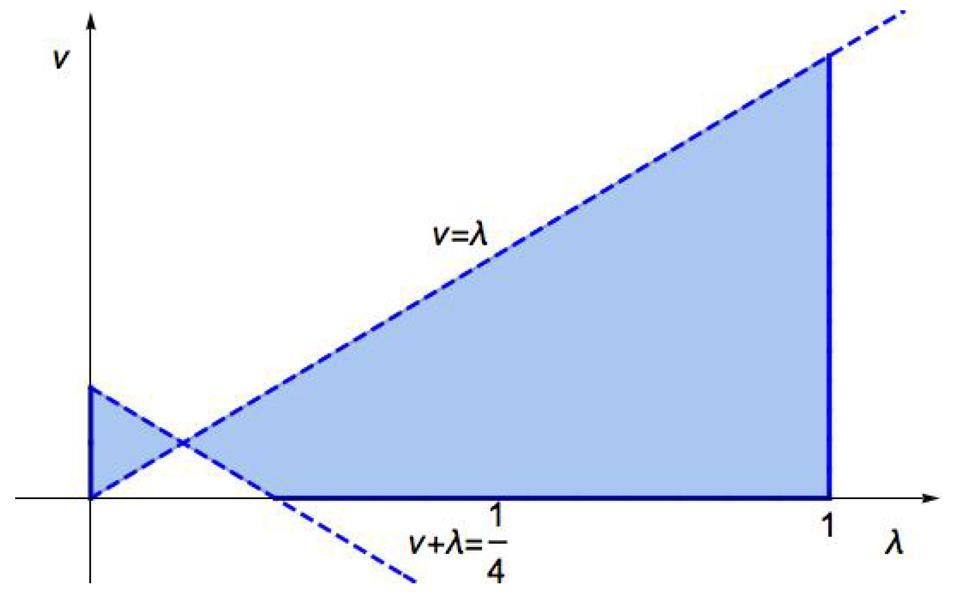
Thus, conditions of $L_2$-stability can be expressed in the form

$$\begin{array}{cc}\hfill & c^4{a}_2^2{a}_1^2\left(a+b{a}_2^2+(1-a-b)a_2^4\right)\left(a+b{a}_1^2+(1-a-b)a_1^4\right)<1,\hfill \\ \hfill & c^6{a}_1^2{a}_2^2{a}_3^2\left(a+b{a}_1^2+(1-a-b)a_1^4\right)\left(k+l{a}_2^2+(1-k-l)a_2^4\right)\hfill \\ \hfill & \times \left(e+d{a}_3^2+(1-e-d)a_3^4\right)\hfill \\ \hfill & +c^6{a}_1^2{a}_2^2{a}_3^2\left(e+d{a}_1^2+(1-e-d)a_1^4\right)\left(a+b{a}_2^2+(1-a-b)a_2^4\right)\hfill \\ \hfill & \times \left(k+l{a}_3^2+(1-k-l)a_3^4\right)\hfill \\ \hfill & +c^4{a}_1^2{a}_3^2\left(e+d{a}_1^2+(1-e-d)a_1^4\right)\left(e+d{a}_3^2+(1-e-d)a_3^4\right)\hfill \\ \hfill & +c^4{a}_2^2{a}_3^2\left(k+l{a}_2^2+(1-k-l)a_2^4\right)\left(k+l{a}_3^2+(1-k-l)a_3^4\right)\hfill \\ \hfill & +c^4{a}_1^2{a}_2^2\left(a+b{a}_1^2+(1-a-b)a_2^4\right)(a+b{a}_1^2+(1-a-b)a_1^4)<1.\hfill \end{array}$$

(28)

The actual boundaries of the information system stability area can be determined in a specific case, see Figure 1.

4.2. Stability of Foreign Currency Exchange Market

The largest market in the world is currently the foreign exchange market, which determines the exchange rates for each currency. The primary function of the foreign exchange market is the transfer of purchasing power from one currency to another. The demand for a country’s currency depends on the country’s balance of payments. In particular, central banks are responsible for maintaining inflation in the interest of sustainable economic growth and, at the same time, contributing to the overall stability of the financial system. A big factor affecting the exchange rates is the interest rate paid by a country’s central bank, the money supply created by the country’s central bank and a country’s economic growth and financial stability. Commercial banks operate in the foreign exchange market, buy and sell currencies for their clients.

A foreign exchange risk arises when a bank holds assets or liabilities in a foreign currency, which causes exchange rate fluctuations and affects the bank’s profit and capital. The actual rates may differ significantly from the trend if drastic changes in the country’s economy occur that may lead to a currency crisis.

The bank’s market activity can be described by system (15). Let the semi-Markov chain in (15) be in three possible states:

• ${\theta }_1$—there is a currency crisis, $a\left({\xi }_k\right)=a_1$,
• ${\theta }_2$—there is a stable foreign currency exchange market, $a\left({\xi }_k\right)=a_2$,
• ${\theta }_3$—there is a market with currency restrictions, $a\left({\xi }_k\right)=a_3$.

If we denote transition intensities as mentioned above in the previous problem, the conditions for the stability of the foreign exchange market will be identical to those obtained there, i.e., (28). In a special case, if

$$a=b=d=e=k=l=\frac{1}{3},$$

(29)

we get the condition of stability in the form

$$\begin{array}{cc}\hfill c^4{a}_2^2{a}_1^2& \left(1+a_2^2+a_2^4\right)\left(1+a_1^2+a_1^4\right)<\frac{1}{9},\hfill \\ \hfill 2c^6{a}_1^2{a}_2^2{a}_3^2\left(1+a_1^2+a_1^4\right)& \left(1+a_2^2+a_2^4\right)\left(1+a_3^2+a_3^4\right)\hfill \\ \hfill +3c^4{a}_1^2{a}_3^2& \left(1+a_1^2+a_1^4\right)\left(1+a_3^2+a_3^4\right)\hfill \\ \hfill +3c^4{a}_2^2{a}_3^2& \left(1+a_2^2+a_2^4\right)\left(1+a_3^2+a_3^4\right)\hfill \\ \hfill +3c^4{a}_1^2{a}_2^2& \left(1+a_1^2+a_2^4\right)(1+a_1^2+a_1^4)<\frac{1}{27}.\hfill \end{array}$$

(30)

The actual boundaries of the foreign exchange market stability area are shown in Figure 1.

4.3. Radiocarbon Dating Modelled by a System with Markov Parameters

The age of an object containing organic material can be determined by using a method called radiocarbon dating. The method is based on the fact that, during its life, a plant or animal is in equilibrium with its surroundings, therefore, it has the same proportion of ${}^{14}C$. When the animal or plant dies, the amount of ${}^{14}C$ it contains begins to decrease and so the ratio of ${}^{14}C$ to ${}^{12}C$ in its remains will gradually decrease. The proportion of radiocarbon can be used to find out when the animal or plant died.

If we denote by k the unit of time, then the amount $X_k$ of radioactive carbon particles ${}^{14}C$ can be expressed by a system of linear difference equations

$$X_{k+1}=A\left({\xi }_k\right)X_k,k=0,1,\dots ,$$

where ${\xi }_k$ is a random Markov chain with two possible states:

• ${\xi }_k={\theta }_1$—the test sample (in terms of detecting age) is not affected by new pollution or the effects of radioactive substances,
• ${\xi }_k={\theta }_2$—the sample process is subject to some kind of influence,

with transition probabilities

$${\pi }_{11}=1-\lambda ,{\pi }_{12}=\nu ,{\pi }_{21}=\lambda ,{\pi }_{22}=1-\nu .$$

The following $2\times 2$ matrices may correspond to these states:

$$\begin{array}{cc}\hfill & A_1=A\left({\theta }_1\right)=\left(\begin{array}{cc}1& 0\\ 0& 1\end{array}\right),\mathrm{if}{\xi }_k={\theta }_1,\hfill \\ \hfill & A_2=A\left({\theta }_2\right)=\left(\begin{array}{cc}0& 1\\ -1& 0\end{array}\right),\mathrm{if}{\xi }_k={\theta }_2,\hfill \end{array}$$

and the moment Equations (24) for the second-order moments obtain the form

$$\begin{array}{cc}\hfill & E_1^{\left(2\right)}\left\{X_{k+1}\right\}=(1-\lambda )\left(\begin{array}{cc}1& 0\\ 0& 1\end{array}\right)E_1^{\left(2\right)}\left\{X_k\right\}\left(\begin{array}{cc}1& 0\\ 0& 1\end{array}\right)+\nu \left(\begin{array}{cc}0& 1\\ -1& 0\end{array}\right)E_2^{\left(2\right)}\left\{X_k\right\}\left(\begin{array}{cc}0& -1\\ 1& 0\end{array}\right),\hfill \\ \hfill & E_2^{\left(2\right)}\left\{X_{k+1}\right\}=\lambda \left(\begin{array}{cc}1& 0\\ 0& 1\end{array}\right)E_1^{\left(2\right)}\left\{X_k\right\}\left(\begin{array}{cc}1& 0\\ 0& 1\end{array}\right)+(1-\nu )\left(\begin{array}{cc}0& 1\\ -1& 0\end{array}\right)E_2^{\left(2\right)}\left\{X_k\right\}\left(\begin{array}{cc}0& -1\\ 1& 0\end{array}\right).\hfill \end{array}$$

Denoting

$$E_1^{\left(2\right)}\left\{X_k\right\}=\left(\begin{array}{cc}{e}_1\left(k\right)& e_2\left(k\right)\\ e_2\left(k\right)& e_3\left(k\right)\end{array}\right),E_2^{\left(2\right)}\left\{X_k\right\}=\left(\begin{array}{cc}{f}_1\left(k\right)& f_2\left(k\right)\\ f_2\left(k\right)& f_3\left(k\right)\end{array}\right),$$

we get the scalar moment equations

$$\begin{array}{cc}\hfill & e_1(k+1)=(1-\lambda )e_1\left(k\right)+\nu f_3\left(k\right),\hfill \\ \hfill & e_2(k+1)=(1-\lambda )e_2\left(k\right)-\nu f_2\left(k\right),\hfill \\ \hfill & e_3(k+1)=(1-\lambda )e_3\left(k\right)+\nu f_1\left(k\right),\hfill \\ \hfill & f_1(k+1)=\lambda f_1\left(k\right)+(1-\nu )e_3\left(k\right),\hfill \\ \hfill & f_2(k+1)=\lambda f_2\left(k\right)-(1-\nu )e_2\left(k\right),\hfill \\ \hfill & f_3(k+1)=\lambda f_3\left(k\right)+(1-\nu )e_1\left(k\right),\hfill \end{array}$$

the characteristic equation for which is in the form

$$\left|\begin{array}{cccccc}z-(1-\lambda )& 0& 0& 0& 0& -\nu \\ 0& z-(1-\lambda )& 0& 0& \nu & 0\\ 0& 0& z-(1-\lambda )& -\nu & 0& 0\\ 0& 0& -(1-\nu )& z-\lambda & 0& 0\\ 0& 1-\nu & 0& 0& z-\lambda & 0\\ -(1-\nu )& 0& 0& 0& 0& z-\lambda \end{array}\right|=0.$$

By calculating the determinant, we get the equation

$${\left(z^2-z-{\lambda }^2+{\nu }^2+\lambda -\nu \right)}^3=0,$$

that has two different roots in the form

$$z=\frac{1}{2}\pm \frac{\sqrt{4{\lambda }^2-4{\nu }^2-4\lambda +4\nu +1}}{2}.$$

The condition $\left|z\right|<1$ holds, if the inequalities

$$0\le 4{\lambda }^2-4{\nu }^2-4\lambda +4\nu +1<1,$$

or, the inequalities

$$\begin{array}{cc}\hfill -{\lambda }^2+{\nu }^2+\lambda -\nu & \le \frac{1}{4},\hfill \\ \hfill {\lambda }^2-{\nu }^2-\lambda +\nu & <0.\hfill \end{array}$$

hold. Thus, we get

$$\begin{array}{cc}\hfill {\left(\nu -\frac{1}{2}\right)}^2-{\left(\lambda -\frac{1}{2}\right)}^2& \le \frac{1}{4},\hfill \\ \hfill {\left(\nu -\frac{1}{2}\right)}^2<{\left(\lambda -\frac{1}{2}\right)}^2.\end{array}$$

The first inequality holds for any $0\le \nu \le 1$ and $0\le \lambda \le 1$.

Then, the stability conditions result directly from the second inequality rewritten into the form

$$(\nu -\lambda )\left(\nu +\lambda -\frac{1}{4}\right)<0,$$

Thus, the process is stable if the probabilities of transition from one state to another satisfy the conditions

$$\left\{\begin{array}{c}\nu <\lambda ,\hfill \\ \nu +\lambda >\frac{1}{4},\hfill \end{array}\right.\mathrm{or}\left\{\begin{array}{c}\nu >\lambda ,\hfill \\ \nu +\lambda <\frac{1}{4}.\hfill \end{array}\right.$$

Under these circumstances, the decay of matter into isotopes is stable. The stability domain is shown in Figure 2.

5. Conclusions

We study a dynamical system under the conditions of uncertainty which are described or are under the influence of a Markov process. The paper’s main contribution is a modified method by which systems of difference equations with random coefficients may be represented by deterministic systems to be investigated using well-known procedures. This modification is based on a suitable definition of stability and on deriving a system of momentum equations for difference equations in which the random parameter depends on a Markov or semi-Markov chain with jumps. The systems considered can be used for the description of a number of real phenomena that may assume an arbitrary finite number of different states.

A Markov process has a strict definition in both the continuous and discrete cases. For example, when a programmer works in the conditions of a hacker attack or its absence, these are two clear states. He can “jump” from one state to another. This means that protection is absent or not with a certain probability. Clear two states mean no drifting (no fluctuation). A special Markov process of the Wiener type might be described as roaming (or fluctuation), which is characteristic, among others, of a drunkard’s walk (with no jumps in such a case). In our problems, we study the stability of the system under conditions of transitions from one state to another by jumping, with history forgotten. Under certain conditions the jump may occur under the influence of some fluctuations. This depends on what definition is given by fluctuation. If fluctuations were investigated as a process that meets all the conditions of a Markov or semi-Markov process, new, interesting results could be derived for further real processes (described, for example, in [15,16]).

In the future, we plan to study the behavior of the system under the influence of processes without memory, as well as combinations of various influences, including those associated with periodic Markov processes to obtain the resonance conditions for solving problems of catastrophe theory, ecology and problems of the oceans. In addition, an infinite number of states of the Markov process is of interest.

There are many practical problems that are modelled by systems of equations of our type with a delayed argument depending on a process that satisfies the Markov property. Therefore, in the future we also plan to apply and justify the methods proposed in the article to systems of equations with random coefficients and a delayed argument.

Having obtained some results for non-linear systems, suitable for practical rather than theoretical applications, we are waiting for a potential demand by people in practical professions.