1. Introduction
Over the last few decades, a lot of progress has been made in developing numerical methods for ordinary differential equations (ODEs), which can produce efficient, reliable and qualitatively correct numerical solutions by preserving some qualitative features of the exact solutions [
1,
2]. This field of research is called geometric numerical integration. In this paper, we are oriented to obtain numerical approximation of Hamiltonian differential equations of the form,
where
H is known as the Hamiltonian or the total energy of the system and
q and
p are generalized coordinates and generalized momenta respectively. The autonomous Hamiltonian systems have two important properties; one is that the total energy remains constant,
The second important property is that the phase flow is symplectic which imply that the motion along the phase curve retains the area of a bounded sub-domain in the phase space. We need such numerical methods which can mimic both properties of the Hamiltonian systems. For this we use symplectic numerical methods to solve system of Equation (
1). The symplectic methods are numerically more efficient than non-symplectic methods for integration over long interval of time [
3]. Among the class of one step symplectic methods, the implicit symplectic Runge–Kutta (RK) methods were developed and presented in [
4].
For general explicit RK methods, it is known that up to order 4, number of stages required in a RK method are equal to the order of the method whereas, for order ≥5, number of stages become greater than the order of the method. Thus for example, an RK method of order 5 needs at least 6 stages and an RK method of order 6 requires at least 17 stages and so on. The more the number of stages are, the more costly the method is.
Butcher [
5] tried to overcome this complexity of order barrier by presenting the idea of effective order. He implemented his idea on RK method of order 5 and was able to construct explicit RK methods of effective order 5 with just 5 internal stages [
5]. Later on, the idea was extended to construct diagonally extended singly implicit RK methods for the numerical integration of stiff differential equations [
6,
7,
8,
9]. Butcher also used the effective order technique on symplectic RK methods for the numerical integration of Hamiltonian systems [
10,
11].
A RK method v has an effective order q if we have another RK method w, known as the starting method, such that has an order q. The method w is used only once in the beginning followed by n iterations of the main method v and the method , known as the finishing method is used only once at the end.
For separable Hamiltonian systems, it is advantageous to solve some components of the differential-equation with one RK method and solve other components of differential equation with another RK method and collectively they are termed as partitioned Runge–Kutta (PRK) methods. We have extended the idea of Butcher to construct symplectic effective order PRK methods which are explicit in nature and hence are less costly than symplectic implicit RK methods. For the effective order PRK methods, we construct two main PRK methods, two starting and two finishing PRK methods such that the two starting methods are applied once at the beginning followed by n iterations of the main PRK methods and the two finishing methods are used at the end.
2. Algebraic Structure of PRK Methods
We are concerned with the numerical solution of separable Hamiltonian systems,
using two s-stages RK methods
and
,
where
and
are the stages for the
u and
v variables,
and
are quadrature weights,
and
are quadrature nodes,
and
are matrices of s-stage PRK methods
M and
, respectively. Here
M is an explicit RK method and
is an implicit RK method. Similarly, we can define two PRK methods
and
, termed as starting methods. The four PRK methods can be represented by Butcher tableaux as,
We need to find the composed methods
and
, which are given by the Butcher tableaux,
The composition asserts to carry out the calculations with starting methods
S and
firstly and applying the PRK methods
M and
to the output. To explain the composition (
3), we consider four PRK methods with two stages each given as,
Solving the differential equation
, we take the first step going from
to
using starting method
S. We then take the second step going from
to
using main method
M. The equations are given as,
The composition
means that we are going from
to
using the composed method
given as,
The Butcher table for the above composed PRK methods is as follows
Similarly, the composition
can be obtained and is represented by the following Butcher table
A numerical scheme has order
p, if after one iteration, the numerical solution matches with the Taylor’s series of the exact solution to the extent that the remainder term has
. The comparison of the numerical solution with the Taylor’s series of the exact solution provides order conditions which must be satisfied to obtain a particular order numerical method. Thus for order 3 method, we have the following order conditions:
3. Rooted Trees for PRK Methods and Order Conditions
There is a graph theoretical approach to study order conditions of RK methods due to Butcher [
12]. We first study the basic concepts from graph theory and then relate the graphs to the order conditions of RK methods.
A graph with non-cyclic representation consisting of vertices and edges with one vertex acting as root is called as rooted tree. The rooted trees whose vertices are either black or white are known as bi-color rooted trees. The trees having black color root is termed as t, while the white rooted trees are represented by . The order of a tree is total number of vertices in a tree. Whereas, the density is the product of number of vertices of a tree and their sub-trees, when we remove the root.
Example 1. Consider a bi-color tree with order 5 and .

The repeated differentiation of Equation (
2) gives
The terms on the right hand side of Equation (13) are called elementary differentials and can be represented graphically with the help of bi-color rooted trees. Thus
k is represented by a black vertex and
r is represented by a white vertex, whereas the differentiation is represented by an edge between two vertices. According to the nature of the differential Equation (
2) in which
k depends only on
v and
r depends only on
u, we only consider trees in which a black vertex has a white child and vice versa [
13]. Such trees are given in
Table 1 and
Table 2. The elementary differentials can be represented by bi-color rooted trees as shown in
Table 3.
The terms on left hand side from Equations (
5)–(
12) are called elementary weights
and
. The elementary weights are nonlinear expressions of the coefficients of PRK methods and can be related to bi-color rooted trees as shown in
Table 3 [
12,
13]. A PRK method is of order
p iff
for all bi-color rooted trees
t and
of order less than or equal to
p [
13].
Let the elementary weight functions of the methods M and are and , respectively such that maps trees t and maps trees to expression in terms of method coefficients as follows

Similarly, we can define elementary weight functions
and
for the starting methods
S and
, respectively. The composition of PRK methods in terms of their elementary weights is
and
given as

where the right hand side of Equation (14) contains terms from
Table 4 which has tree
u as a sub-tree of tree
t and
is the remaining tree when
u is removed from
t.
The order condition related to the tree

for the composed method (
4) is

4. Effective Order PRK Methods
Let
M and
S be two RK methods together with an inverse method
. The effective order
q means that the composition
has order
q [
6]. For PRK methods, we are interested to construct methods
M,
,
S,
together with the inverse methods
and
such that the compositions
and
have the effective order
q which implies
and
for all trees of order
q [
12], where
E is the exact flow for which corresponding order conditions are satisfied. The terms are given in
Table 1 and
Table 2.
A method of effective order 3 is obtained by comparing two columns of
Table 1 and
Table 2 each for trees up to order 3. Thus we have
By eliminating
and
values, Equations (19)–(22) become
5. Symplectic PRK Methods with Effective Order 3
The flow of a Hamiltonian system (
2) is symplectic and it is a well known fact that the discrete flow by symplectic Runge-Kutta methods is symplectic [
14]. The PRK method
M and
for separable Hamiltonian system (
2) is symplectic if the following condition is satisfied [
14]
Moreover, the composition of two symplectic RK methods is symplectic [
10,
15].
For symplectic PRK methods, the trees related to order conditions can be divided into superfluous and non-superfluous bi-color trees. Unlike RK methods, the superfluous bi-color trees of PRK methods also contribute one order condition together with one condition from non-superfluous bi-color tree [
14]. Since, the underlying bi-color tree of the rooted trees
and
is superfluous. So, we can ignore the condition (18) because it is automatically satisfied. Moreover, the underlying bi-color trees of
,
,
and
are non-superfluous, we can either take
or
and also
or
resulting in reducing Equations (23) and (24) to
and
. Now consider the following Butcher table for methods
M and
which satisfy the symplectic condition (25)
The Equations (15)–(17) and (23)–(24) after simplification can be written in terms of elementary weights as
To get the values of 6 unknowns from 5 equations, we have one degree of freedom. Let us take
and solve Equations (27)–(31) to get
M and
methods as follows
Derivation of Starting Method
For the starting method, we have the following equations
The starting methods should be symplectic [
16]. The solution of (32)–(35) leads us to the following symplectic staring PRK methods
S and
as
6. Mutually Adjoint Symplectic Effective Order PRK Methods
A separable Hamiltonian system remains unchanged by changing the role of kinetic and potential energies, position, and momentum and also inverting the direction of time. For the two PRK method tableaux (26) being mutually adjoint, we have
,
and
in Equations (27)–(31), so we have
Sanz-Serna suggested in [
14] to take
= 0.91966152, which leads us to the following main methods
M and
with effective order 3 with just 3 stages
The starting methods
S and
for mutually adjoint symplectic effective order PRK method are constructed by using
,
,
in Equations (32) to (34) to get
By solving Equations (40) and (41) with
, we get the following
S and
methods:
7. Numerical Experiments
The symplectic RK methods should be implicit and hence their computational cost is higher due to large number of function evaluations. On the other hand, we can use symplectic explicit PRK methods for Hamiltonian systems with lesser computational cost because of the explicit nature of the stages. Our derived effective order symplectic PRK methods are explicit and we have used MATLAB to implement them on Hamiltonian systems for the energy conservation and order confirmation of these methods.
7.1. Kepler’s Two Body Problem
Consider Kepler’s two body problem given as
where
. The energy is given by,
The exact solution after half revolution is
To verify the effective order 3 behavior, we apply the starting methods
S and
to perturb initial values to
,
and
,
, respectively. Then we apply the main methods
M and
for
n number of iterations to
,
and
,
, respectively and obtain the numerical solutions
,
and
,
computed at
where
h is the step-size. We then evaluate exact solutions at
to get
,
and
,
and perturb them using starting methods
S and
to obtain
,
and
,
. Finally, to obtain global error, we take the difference between numerical and exact solutions, i.e.,
. Effective order 3 behavior for symplectic and mutually adjoint symplectic PRK is confirmed from
Table 5 and
Table 6.
We calculate the ratio of global errors calculated at step length
h,
,
and
. For method of order
p, ratio should approximately be
[
12].
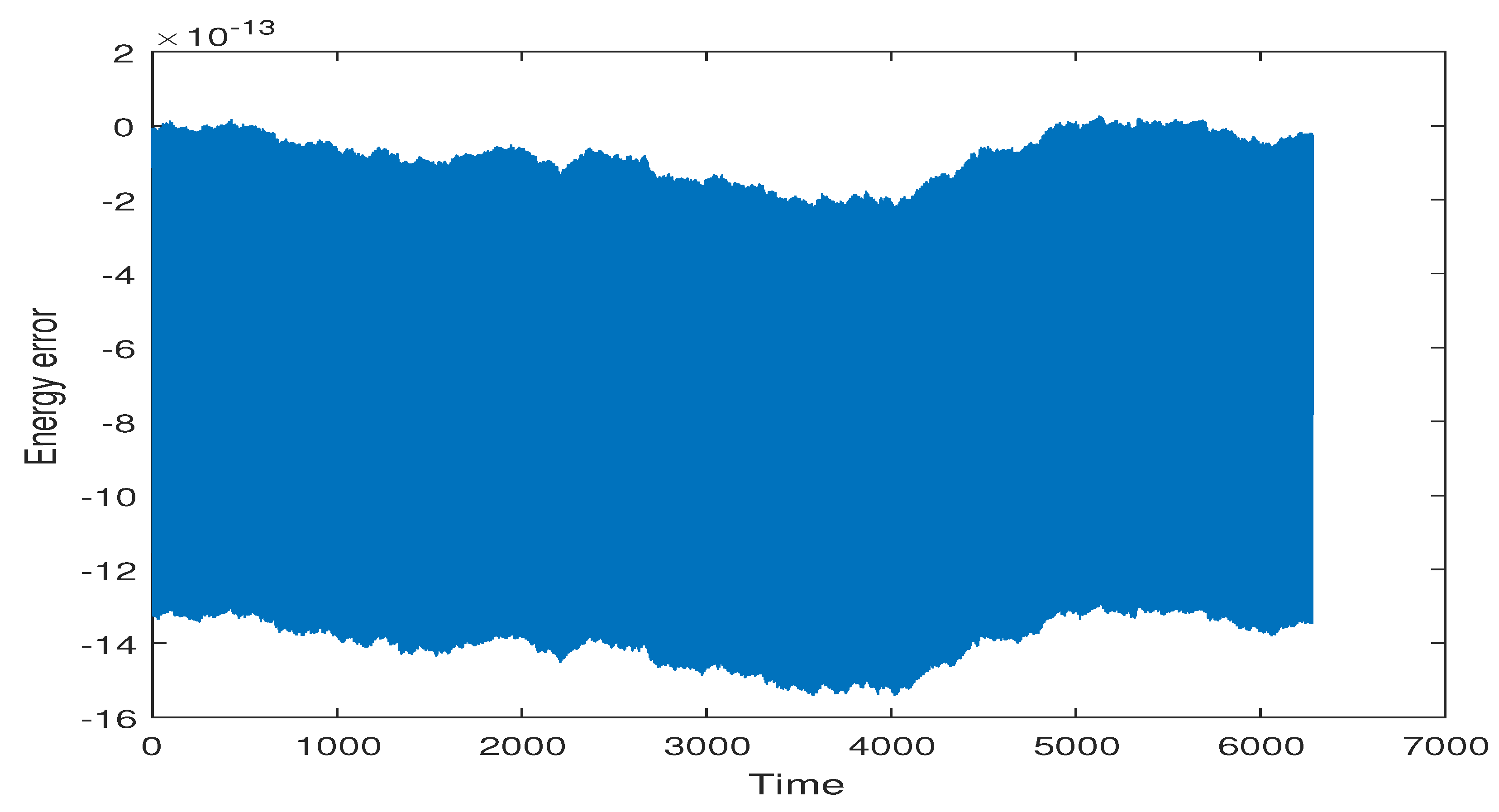
The next experiment is to verify the energy conservation behaviour of the symplectic methods. In this experiment, the step-size
is used for
iterations.
Figure 1 and
Figure 2 depict good conservation of energy with symplectic and mutually adjoint symplectic effective order PRK methods, respectively. Whereas, the energy error was bounded above by
and
, respectively.
7.2. Harmonic Oscillator
The motion of a unit mass attached to a spring with momentum
u and position co-ordinates
v defines the Hamiltonian system
We have applied the symplectic PRK and mutually adjoint symplectic PRK methods with step-size
with
iteration in this experiment. We have obtained good energy conservation as shown in
Figure 3 and
Figure 4 by symplectic effective order PRK and mutually adjoint symplectic effective order PRK methods, respectively.
8. Conclusions
In this paper, the composition of two PRK methods is elaborated in terms of Butcher tableaux as well as in terms of their elementary weight functions. The effective order conditions are provided for PRK methods and 3 stage effective order 3 symplectic PRK methods are constructed and successfully applied to separable Hamiltonian systems with good energy conservation. It is worth mentioning that we are able to construct mutually adjoint symplectic effective order 3 PRK methods with just 3 stages, whereas an equivalent method of order 3 with 4 stages is given in [
16]. In dynamical solar systems, we deal with many problems which are described by Hamiltonian systems, like, Kepler’s two body problem and more realistic Jovian five body problem. These symplectic methods are much useful for such types of physical phenomena to observe their positions and energy conservation.
Author Contributions
Formal analysis, J.A., A.A., S.S. and M.Y.; investigation, J.A., Y.H., S.u.R., A.A. and S.S.; software, J.A., Y.H., S.u.R. and M.Y.; validation, J.A.; writing—original draft, J.A.; writing—review & editing, Y.H., S.u.R. and S.S.; conceptualization, Y.H.; methodology Y.H. and S.S.; Supervision, Y.H. and S.u.R.; visualization, Y.H., A.A. and M.Y.; resources, S.S. and M.Y.
Funding
This research received no external funding.
Conflicts of Interest
The authors declare no conflict of interest.
References
- Sanz-Serna, J.M.; Calvo, M.P. Numerical Hamiltonian Problems; Chapman & Hall: London, UK, 1994. [Google Scholar]
- Blanes, S.; Moan, P.C. Practical symplectic partitioned Runge–Kutta and Runge–Kutta–Nyström methods. J. Comput. Appl. Math. 2002, 142, 313–330. [Google Scholar] [CrossRef]
- Chou, L.Y.; Sharp, P.W. On order 5 symplectic explicit Runge-Kutta Nyström methods. Adv. Decis. Sci. 2000, 4, 143–150. [Google Scholar] [CrossRef]
- Geng, S. Construction of high order symplectic Runge-Kutta methods. J. Comput. Math. 1993, 11, 250–260. [Google Scholar]
- Butcher, J.C. The effective order of Runge–Kutta methods. Lecture Notes Math. 1969, 109, 133–139. [Google Scholar]
- Butcher, J.C. Order and effective order. Appl. Numer. Math. 1998, 28, 179–191. [Google Scholar] [CrossRef]
- Butcher, J.C.; Chartier, P. A generalization of singly-implicit Runge-Kutta methods. Appl. Numer. Math. 1997, 24, 343–350. [Google Scholar] [CrossRef]
- Butcher, J.C.; Chartier, P. The effective order of singly-implicit Runge-Kutta methods. Numer. Algorithms 1999, 20, 269–284. [Google Scholar] [CrossRef]
- Butcher, J.C.; Diamantakis, M.T. DESIRE: Diagonally extended singly implicit Runge—Kutta effective order methods. Numer. Algorithms 1998, 17, 121–145. [Google Scholar] [CrossRef]
- Butcher, J.C.; Imran, G. Symplectic effective order methods. Numer. Algorithms 2014, 65, 499–517. [Google Scholar] [CrossRef]
- Lopez-Marcos, M.; Sanz-Serna, J.M.; Skeel, R.D. Cheap Enhancement of Symplectic Integrators. Numer. Anal. 1996, 25, 107–122. [Google Scholar]
- Butcher, J.C. Numerical Methods for Ordinary Differential Equations, 2nd ed.; Wiley: Hoboken, NJ, USA, 2008. [Google Scholar]
- Hairer, E.; Nørsett, S.P.; Wanner, G. Solving Ordinary Differential Equations I for Nonstiff Problems, 2nd ed.; Springer: Berlin, Germany, 1987. [Google Scholar]
- Sanz-Serna, J.M. Symplectic integrators for Hamiltonian problems. Acta Numer. 1992, 1, 123–124. [Google Scholar] [CrossRef]
- Habib, Y. Long-Term Behaviour of G-symplectic Methods. Ph.D. Thesis, The University of Auckland, Auckland, New Zealand, 2010. [Google Scholar]
- Butcher, J.C.; D’Ambrosio, R. Partitioned general linear methods for separable Hamiltonian problems. Appl. Numer. Math. 2017, 117, 69–86. [Google Scholar] [CrossRef]
© 2019 by the authors. Licensee MDPI, Basel, Switzerland. This article is an open access article distributed under the terms and conditions of the Creative Commons Attribution (CC BY) license (http://creativecommons.org/licenses/by/4.0/).

 ,
, 

 where the right hand side of Equation (14) contains terms from Table 4 which has tree u as a sub-tree of tree t and is the remaining tree when u is removed from t.
 for the composed method (4) is


