Nonlinear Dynamic Modelling of Two-Point and Symmetrically Supported Pipeline Brackets with Elastic-Porous Metal Rubber Damper

Abstract

This paper aims to investigate the nonlinear dynamic properties of a two-point and symmetrically supported pipeline bracket system coated with the damping element using an elastic-porous metal rubber. The dynamic model of the studied two-point and symmetric pipeline system was established based on impulse response matrix for accurate and reliable description on its nonlinear behaviours, e.g., energy dissipation and loss factor. The experimental verification of the developed model was performed by means of dynamic test as well as the analyses of nonlinear damping characteristics. The experimental results show a good agreement with the prediction results obtained from the proposed dynamic model. This work provides an alternative method to investigate the dynamics of pipeline vibration system equipped with a damping structure.

1. Introduction

Flexible and vibrating structures of pipeline system are ubiquitous in extensive engineering areas and industrial applications of civil, aerospace, marine and so on. These structures can experiment harmful vibrations resulting from its interaction with the environment, as resonance and flutter oscillations, that if are not correctly controlled, can lead to undesirable noise and even the collapsing of the structure. In this scenario, the use of feasible damping materials for vibration control is an attractive option to mitigate such vibrations. Modelling and/or control of such damping vibration systems with nonlinear dynamic behaviours should be a challenge due to the complexity of the characteristic polynomial.

Many researchers have extensively attempted to establish dynamic models and analyse the vibration characteristics in terms of various pipeline systems. Li et al. [1] proposed a semi-analytical method base on the He’s variational iteration method to analyse the conservative free vibration problem of conveying fluid pipe. For almost the similar pipeline system, Zhou et al. [2] considered the cantilevered fluid-transporting pipe as a non-conservative system and developed a model control strategy involving the mass, damping, stiffness and suppression region using the idea of nonlinear energy sink. Zhang et al. [3] provided a feasible solution for the nonlinear vibration problem of a fluid-conveying pipeline system with general boundary working conditions, in which the pipeline could be divided into the straight pipe and the bent pipe. Rong et al. [4] analysed the dynamics of flexible beams with large deformations via the absolute nodal coordinate transfer matrix method. Some other scholars focused on the control strategies of vibration reduction associated with the nonlinear dynamics of fluid conveying curved pipeline systems [5,6,7,8,9]. The pipeline systems with two-point and symmetrically supported brackets are widely applied in some precise apparatus and have also made some efforts in the past decade. For example, Modarres-Sadeghi et al. [10] attempted to explore the dynamic characteristics of straight pipes which were supported at both ends. However, the previous efforts have tended to focus on the rigidly supported pipeline system or linear vibration, rather than on the elastic support with damping performance.

In the view of pipeline vibration system considering damping structure, some efforts on the theoretic model have been made in terms of individual cases. Amabili et al. [11] studied the nonlinear damping performance under large amplitude conditions and proposed a fractional linear solid model with the geometrically nonlinear viscoelasticity. Kong et al. [12] attempted to explore the effects of damping, the dynamical behaviours of coupled systems of nonlinear energy sink (NES) including the bifurcations and strongly modulated regimes. In particular, the influence of a 2-dof NES on the response regimes and performance of vibration suppression was analysed in detail. Rezaiee-Pajand and Sarafrazi [13] introduced a novel dynamic relaxation method with zero damping terms. They indicated that a proper time-step ratio is able to guarantee the convergence of the proposed model. Zhai et al. [14] reported that the active constrained layer damping treatment was adopted to investigate the vibration control of an aero pipeline system in terms of the vibration and stress distribution. Furthermore, a three-dimensional finite element model of such a pipeline with active constrained layer damping (ACLD) patches was developed. Recently, there has been growing interest in the high static and low dynamic characteristics with a geometric nonlinear damping system. For example, a novel design of the geometric nonlinear damping (GND) was presented to enhance the vibration isolation performance of the high-static—low-dynamic stiffness (HSLDS) isolator under both base and force excitations [15]. The nonlinear dynamic stability of Euler-Bernoulli beam-columns with damping structure was investigated by combining the analytical and numerical methods [16]. Wang et al. utilized Riccati discrete time transfer matrix method to analyse the dynamics of an underwater towed system and prove its capability [17]. Some researchers further applied Riccati discrete time transfer matrix method to analyse the nonlinear dynamics of pipeline system [18,19]. Their results indicate that dynamic relaxation methods can be an effective nonlinear dynamic analysis method for the truss and frame structures.

However, there is no comprehensive research so far available to well describe the nonlinear dynamic characteristics of the supported pipeline system that contains a damping structure. Elastic-porous metal rubber, also known as entangled wire mesh, exhibits typical nonlinear characteristics with a hysteresis loop of displacement-force curve under dynamic loading conditions [20,21,22,23]. It has been proved to effectively reduce the transmission of vibration in a variety of industrial structures such as coated structure [24], smart rotor support [25] and the pipeline systems [26]. Wu et al. [24] designed a new coated structure with large-size metal rubber bellows and investigated the energy dissipation characteristics. Their results indicated that the dynamic vibration characteristics coated structure with large-size metal rubber bellows has great dependence on the vibration amplitude and frequency. Ma et al. [25] designed a smart rotor support with shape memory alloy metal rubber (SMA-MR) and studied the mechanical performance of smart rotor support with SMA-MR under high temperature variable amplitude vibrations. The results revealed that the smart rotor support with SMA-MR can provide variable stiffness and damping characteristics with temperature, excitation amplitude and frequency. Kwon et al. [26] developed a ring-type SMA mesh washer isolator that can be used in both launch vibration and on-orbit micro-jitter environments without requiring a launch lock device. The manufacturing processes of metal rubber generally include several steps including encircled tight helix, coiled wire with a particular pitch, a rough blank in a crisscross pattern, press formation and post-treatment [27,28].

The objective of this paper is to analyse the dynamic properties of the two-point and symmetrically supported pipeline system coated with a damping structure (elastic-porous metal rubber) and establish the dynamic model for the two-point and symmetrically supported pipeline brackets. The nonlinear dynamic analysis of long and straight pipeline with low-order modes can be performed as well as the experimental verification of the developed dynamic model. In Section 2, the simplification of the physical model of vibration isolation system for two-point and symmetrically supported pipeline brackets is introduced. In Section 3, the dynamic model based on impulse response matrix for accurate and reliable description on its nonlinear behaviors is established. In Section 4, the experiment for two-point and symmetrically supported pipeline brackets under different excitation conditions are carried out to analyze the nonlinear characteristics of the coated pipeline system. In Section 5, the main conclusions of this paper are drawn.

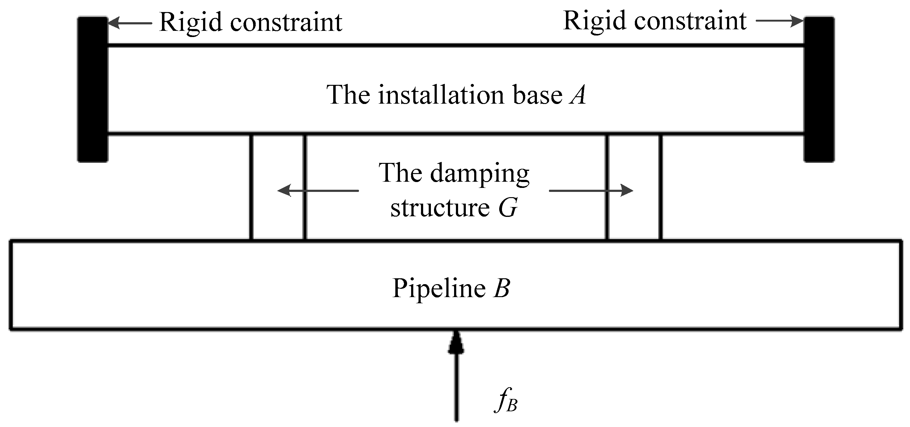
2. Description of Pipeline Vibration Isolation System

For the pipeline coated system, due to the modal characteristics of the long pipeline and thin-plate installation base, the whole pipeline system can be regarded as a physical structure of active vibration isolation. As shown in Figure 1, the pipeline B that connected with the installation base A through the coated damping structure G (the support) is subjected to external excitation force f_B, which can be weakened through the coated damping G. Thus, the pipeline system is able to realize the purpose of the vibration reduction.

In this paper, the damping structure G contains metal rubber, and pipeline B connected with installation base A through the two-point and symmetrically supported pipeline brackets. Based on these assumptions, the studies of the dynamics for the coated pipeline system were performed.

2.1. Model Simplifications

To install the installation base A with concrete size, simplifying the installation base A can be simplified as a regular elastic support with uniform thickness and considered as a uniform rectangular plate (a × b). The material properties of the installation base A mainly include elastic modulus E_A, Poisson’s ratio μ_A, density ρ_A, etc. As a result of the restraint mode of the installation base A that is supported and fixed at both ends, it has only an elastic mode and no rigid body displacement.

The pipeline B can be simplified as a geometric structure with length c, and the external diameter d. For its material properties, the pipeline B has specific mechanical behaviours, such as elastic modulus E_B, Poisson’s ratio μ_B, density ρ_B, etc. The pipeline B connected on the installation base A by the coated damping structure G in a manner using the two-point and symmetrically supported brackets which have elastic and rigid modes when it is suffered by an external excitation.

In terms of the coordinate system, the earth is chosen and set as the absolute coordinate system, and the left side of the installation base A is considered as the origin of the coordinate system.

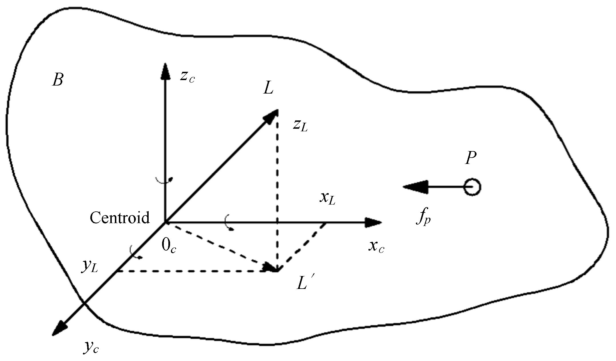
2.2. Junction Definition

A corresponds relationship is established one by one between the connection point on the installation base A, and the connection point on the pipeline B are denoted as A_i (I = 1, 2) and B_i (I = 1, 2), respectively. It is assumed that the coated damping structure has three-dimensional (x, y, z) stiffness and damping characteristics. The isotropic mechanical behaviours are also assumed with the same stiffness and damping characteristics in the three directions.

For the installation base A, the set of connection degrees of freedom I is defined as:

$$\{x_{A_1},y_{A_1},z_{A_1}\},\{x_{A_2},y_{A_2},z_{A_2}\},\{f{x}_{A_1},f{y}_{A_1},f{z}_{A_1}\},\{f{x}_{A_2},f{y}_{A_2},f{z}_{A_2}\}$$

For the pipeline B, the set of connection degrees of freedom J can be denoted as follows:

$$\{x_{B_1},y_{B_1},z_{B_1}\},\{x_{B_2},y_{B_2},z_{B_2}\},\{f{x}_{B_1},f{y}_{B_1},f{z}_{B_1}\},\{f{x}_{B_2},f{y}_{B_2},f{z}_{B_2}\}$$

Based on the above two definitions, the set of connection degrees of freedom I is in one-to-one correspondence with that of J, and the number of degrees of freedom for both A and B is 6. $\{x_{A_i},y_{A_i},z_{A_i}\}$, $\{x_{B_i},y_{B_i},z_{B_i}\}$ correspond to the absolute displacement components of the connecting points $\{A_i,B_i\}$ respectively; $\{f{x}_{A_i},f{y}_{A_i},f{z}_{A_i}\}$, $\{f{x}_{B_i},f{y}_{B_i},f{z}_{B_i}\}$ represent the components of the connecting force applied to A and B at the connecting points $\{A_i,B_i\}$; $\{-f{x}_{A_i},-f{y}_{A_i},-f{z}_{A_i}\}$, $\{-f{x}_{B_i},-f{y}_{B_i},-f{z}_{B_i}\}$ represent the component of force applied to the coated damping structure G at the connecting points $\{A_i,B_i\}$.

For the absolute displacement component, a relation generally exists as follows:

$$\{x_{A_i},y_{A_i},z_{A_i}\}\ne \{x_{B_i},y_{B_i},z_{B_i}\}\left(i=1,2\right)$$

(1)

This can be attributed to the elastic connection between installation base A and pipeline B, which leads to the existence of relative displacement between freedom I and J. The relationship between acting force and reaction force between joints is then given by the following relation:

$$\{f{x}_{A_i},f{y}_{A_i},f{z}_{A_i}\}=-\{f{x}_{B_i},f{y}_{B_i},f{z}_{B_i}\}.\left(i=1,2\right)$$

(2)

3. Dynamic Modelling

Based on the above model simplification and junction definition, the dynamic model can be established by analysing the two-point elastic partial impulse response function matrix in this section. Firstly, the mathematical model of elastic partial impulse response function matrix on I and J is put forward respectively. Then, response analysis of arbitrary points on A and B caused by connecting force is provided. Finally, the dynamic model of two-point and symmetrically supported pipeline brackets with elastic-porous metal rubber damper is proposed.

3.1. Elastic Partial Impulse Response Function Matrix on I

For the viscous damped n_A DOF discrete vibration system with installation base A, the differential equation of motion can be written as follows:

$$M_A{\ddot{x}}_A+C_A{\dot{x}}_A+K_A{x}_A=f_A(t).$$

(3)

where, $M_A,C_A,K_A\in R^{n_A\times n_A}$; n_A is the set of discrete degree of freedom (I ∈ n_A) of the installation base A; $f_A(t)$ is the external excitation (including connection force $\{f{x}_{A_i},f{y}_{A_i},f{z}_{A_i}\},\left(i=1,2\right)$, column vector on n_A; ${\ddot{x}}_A$, ${\dot{x}}_A$ and $x_A$ correspond to the acceleration, velocity and displacement column vectors on the set of discrete degrees of freedom n_A, respectively.

At present, the main work is to find the elastic partial impulse response function matrix on I. Thus, only the external excitation (the connection force) on I is considered and the $f_A(t)$ is given by

$$f_A(t)\in R^{n_A\times 1}={\{0,\cdots ,f{x}_{A_1},f{y}_{A_1},f{z}_{A_1},\cdots ,f{x}_{A_2},f{y}_{A_2},f{z}_{A_2},\cdots 0\}}^{\mathrm{T}}.$$

(4)

The position $n_A\left\{f{x}_{A_1}\right\}$ of mark $f{x}_{A_1}$ in $f_A(t)$ is denoted as ${\tilde{n}}_{1A}$, then $n_A\left\{f{y}_{A_1}\right\}={\tilde{n}}_{1A}+1$, $n_A\left\{z{y}_{A_1}\right\}={\tilde{n}}_{1A}+2$. Similarly, the position $n_A\left\{f{x}_{A_2}\right\}$ of mark $f{x}_{A_2}$ in $f_A(t)$ is expressed as, ${\tilde{n}}_{2A}$, then $n_A\left\{f{y}_{A_2}\right\}={\tilde{n}}_{2A}+1$, $n_A\left\{z{y}_{A_2}\right\}={\tilde{n}}_{2A}+2$.

In the same manner, the velocity and the displacement for the column vectors of acceleration on the set of discrete degrees of freedom n_A. They can be expressed as:

$$x_A\in R^{n_A\times 1}={\{\cdots ,x_{A_1},y_{A_1},z_{A_1},\cdots ,x_{A_2},y_{A_2},z_{A_2},\cdots \}}^{\mathrm{T}}$$

(5a)

$${\dot{x}}_A\in R^{n_A\times 1}={\{\cdots ,{\dot{x}}_{A_1},{\dot{y}}_{A_1},{\dot{z}}_{A_1},\cdots ,{\dot{x}}_{A_2},{\dot{y}}_{A_2},{\dot{z}}_{A_2},\cdots \}}^{\mathrm{T}}$$

(5b)

$${\ddot{x}}_A\in R^{n_A\times 1}={\{\cdots ,{\ddot{x}}_{A_1},{\ddot{y}}_{A_1},{\ddot{z}}_{A_1},\cdots ,{\ddot{x}}_{A_2},{\ddot{y}}_{A_2},{\ddot{z}}_{A_2},\cdots \}}^{\mathrm{T}}$$

(5c)

$$n_A\left\{x_{A_i}\right\}=n_A\left\{{\dot{x}}_{A_i}\right\}=n_A\left\{{\ddot{x}}_{A_i}\right\}={\tilde{n}}_{iA}\left(i=1,2\right)$$

(6)

Considering the consistency of finite element analysis and modal experimental analysis for A, it is suggested that the two methods should have combined in an identical way. Each grid node is described by $\{x,y,z\}$ coordinate (degree of freedom) and labelled continuously according to node and order of $x\to y\to z$. In this case, ${\tilde{n}}_{iA}$ can be determined uniquely. Then, block matrix is introduced as follows:

$$R=\left[\begin{array}{ccc}{C}_A& \cdots & M_A\\ ⋮& & ⋮\\ M_A& \cdots & 0\end{array}\right],S=\left[\begin{array}{ccc}{K}_A& \cdots & 0\\ ⋮& & ⋮\\ 0& \cdots & -M_A\end{array}\right],y=\left\{\begin{array}{c}{x}_A\\ ⋮\\ {\dot{x}}_A\end{array}\right\},z^{\prime }=\left\{\begin{array}{c}{f}_A(t)\\ ⋮\\ 0\end{array}\right\}$$

(7)

Equation (3) is algebraically treated according to Equation (7) and solved by homogeneous breeze equation. Then, its eigenvalues are obtained as well as feature vectors, marked as ${\lambda }_1$, ${\lambda }_2$, …, ${\lambda }_{n_A}$, ${\lambda }_1^{*}$, ${\lambda }_2^{*}$, …, ${\lambda }_{n_A}^{*}$, and ${\phi }_1^{\prime }$, ${\phi }_2^{\prime }$, …, ${\phi }_{nA}^{\prime }$, ${{\phi }_1^{\prime }}^{*}$, ${{\phi }_2^{\prime }}^{*}$, …, ${{\phi }_{nA}^{\prime }}^{*}$ respectively.

By solving the equation and transforming some columns, the displacement expression of the system in the physical coordinate system under the zero initial condition is obtained as:

$$x_A(t)={\displaystyle \sum _{i=1}^{n_A}}\{\frac{{\phi }_i{\phi }_i^{\mathrm{T}}}{a_i}{\int }_0^t{\mathrm{e}}^{{\lambda }_i(t-\tau )}{f}_A(\tau )\mathrm{d}\tau +\frac{{\phi }_i^{*}{\phi }_i^{\mathrm{H}}}{a_i^{*}}{\int }_0^t{\mathrm{e}}^{{\lambda }_i^{*}(t-\tau )}{f}_A(\tau )\mathrm{d}\tau \}.$$

(8)

where a_i, called complex mode mass, is consistent with the expression of natural frequency. By applying Laplacian transformation on both sides of Equation (8) and using the properties of convolution Laplacian transformation, Equation (8) can be further transformed into:

$$L[x_A(t)]=X_A(s)={\displaystyle \sum _{i=1}^{n_A}}\{\frac{{\phi }_i{\phi }_i^{\mathrm{T}}}{a_i(s-{\lambda }_i)}+\frac{{\phi }_i^{*}{\phi }_i^H}{a_i^{*}(s-{\lambda }_i^{*})}\}L[f_A(t)].$$

(9)

In order to solve the transfer function matrix from I to the whole A, a series of transformations are requested for Equation (9). They mainly include expanding and extracting the elements in $f_A(t)$ of Equation (9) to form a new matrix ${\tilde{f}}_A(t)$, and the concept of ${\phi }_{Ii}$, ${\phi }_{Ii}^{*}$. Therefore,

$$\left\{\frac{{\phi }_i{\phi }_i^{\mathrm{T}}}{a_i(s-{\lambda }_i)}+\frac{{\phi }_i^{*}{\phi }_i^{\mathrm{H}}}{a_i^{*}(s-{\lambda }_i^{*})}\right\}L[f_A(t)]=\left\{\frac{{\phi }_i{\phi }_{Ii}^{\mathrm{T}}}{a_i(s-{\lambda }_i)}+\frac{{\phi }_i^{*}{\phi }_{Ii}^{\mathrm{H}}}{a_i^{*}(s-{\lambda }_i^{*})}\right\}L[{\tilde{f}}_A(t)].$$

(10)

where ${\phi }_{Ii}$, ${\phi }_{Ii}^{*}$ represent the components of ${\phi }_i$, ${\phi }_i^{*}$ on the mode vector, respectively. By substituting Equation (10) into Equation (9), one obtains:

$$L[x_A(t)]=X_A(s)={\displaystyle \sum _{i=1}^{n_A}}\left\{\frac{{\phi }_i{\phi }_{Ii}^{\mathrm{T}}}{a_i(s-{\lambda }_i)}+\frac{{\phi }_i^{*}{\phi }_{Ii}^{\mathrm{H}}}{a_i^{*}(s-{\lambda }_i^{*})}\right\}L[{\tilde{f}}_A(t)].$$

(11)

In this case, the transfer function matrix from I to the whole A can be obtained as:

$$H_{AI}(s)=\frac{X_A(s)}{L[{\tilde{f}}_A(t)]}=\frac{X_A(s)}{{\tilde{F}}_A(s)}={\displaystyle \sum _{i=1}^{n_A}}\left\{\frac{{\phi }_i{\phi }_{Ii}^{\mathrm{T}}}{a_i(s-{\lambda }_i)}+\frac{{\phi }_i^{*}{\phi }_{Ii}^{\mathrm{H}}}{a_i^{*}(s-{\lambda }_i^{*})}\right\}.$$

(12)

Based on Equation (12), the impulse response function matrix from I to the whole A can be derived as:

$$h_{AI}(t)={\displaystyle \sum _{i=1}^{n_A}}\frac{{\phi }_i{\phi }_{Ii}^{\mathrm{T}}}{a_i}{\mathrm{e}}^{{\lambda }_{i}t}+\frac{{\phi }_i^{*}{\phi }_{Ii}^{\mathrm{H}}}{a_i^{*}}{\mathrm{e}}^{{\lambda }_i^{*}t}.$$

(13)

By expanding, the Equation (11) can be transformed into:

$$\begin{array}{c}L{\{\cdots ,x_{A_1},y_{A_1},z_{A_1},\cdots ,x_{A_2},y_{A_2},z_{A_2},\cdots \}}^{\mathrm{T}}\hfill \\ ={\displaystyle \sum _{i=1}^{n_A}}\left\{\frac{1}{a_i(s-{\lambda }_i)}\{\begin{array}{cccc}{\phi }_i{\phi }_{Ii1}& {\phi }_i{\phi }_{Ii2}& \cdots & {\phi }_i{\phi }_{Ii6}\end{array}\}+\frac{1}{a_i^{*}(s-{\lambda }_i^{*})}\{\begin{array}{cccc}{\phi }_i^{*}{\phi }_{Ii1}^{*}& {\phi }_i^{*}{\phi }_{Ii2}^{*}& \cdots & {\phi }_i^{*}{\phi }_{Ii6}^{*}\end{array}\}\right\}{\tilde{F}}_A(s).\hfill \end{array}$$

(14a)

Similarly, we extracted and reorganized the $\{{\tilde{n}}_{iA},{\tilde{n}}_i{}_A+2\},\left(i=1,2\right)$ element in $x_A(t)$ to obtain a new displacement column vector ${\tilde{x}}_A(t)$ on I, that is

$${\tilde{x}}_A(t)={\{x_{A_1},y_{A_1},z_{A_1},x_{A_2},y_{A_2},z_{A_2}\}}^{\mathrm{T}}.$$

(14b)

Based on Equations (14a) and (14b), the $I\to I$ impulse response function matrix $h_{II}(t)$ can be derived as:

$$\begin{array}{cc}{h}_{II}(t)& =L^{-1}[H_{II}(s)]=L^{-1}\left[\frac{{\tilde{X}}_A(s)}{{\tilde{F}}_A(s)}\right]\hfill \\ & =L^{-1}\left[{\displaystyle \sum _{i=1}^{n_A}}\left\{\frac{{\phi }_{Ii}{\phi }_{Ii}^{\mathrm{T}}}{a_i(s-{\lambda }_i)}+\frac{{\phi }_{Ii}^{*}{\phi }_{Ii}^{\mathrm{H}}}{a_i^{*}(s-{\lambda }_i^{*})}\right\}\right]={\displaystyle \sum _{i=1}^{n_A}}\frac{{\phi }_{Ii}{\phi }_{Ii}^{\mathrm{T}}}{a_i}{\mathrm{e}}^{{\lambda }_{i}t}+\frac{{\phi }_{Ii}^{*}{\phi }_{Ii}^{\mathrm{H}}}{a_i^{*}}{\mathrm{e}}^{{\lambda }_i^{*}t}.\hfill \end{array}$$

(15a)

Due to the necessity of distinguishing the parameters A and B, $a_i\to a_{Ai}$, ${\lambda }_i\to {\lambda }_{Ai}$, $a_i^{*}\to a_{Ai}^{*}$, ${\lambda }_i^{*}\to {\lambda }_{Ai}^{*}$ are introduced, and Equation (15a) can be rewritten as:

$$h_{II}(t)={\displaystyle \sum _{i=1}^{n_A}}\frac{{\phi }_{Ii}{\phi }_{Ii}^{\mathrm{T}}}{a_{Ai}}{e}^{{\lambda }_{Ai}t}+\frac{{\phi }_{Ii}^{*}{\phi }_{Ii}^{\mathrm{H}}}{a_{Ai}^{*}}{e}^{{\lambda }_{Ai}^{*}t}.$$

(15b)

3.2. Impulse Response Function Matrix on J

The pipeline B and installation base A elastically connected each other by the coated damping structure G in a manner of two-point and symmetrically supported brackets which have elastic and rigid modes when they are suffered external excitation. Then, elastic modes are analysed firstly. The differential equation of motion for the viscous damped n_B DOF discrete vibration system of B can be achieved according to the analysis of A as follows:

$$M_B{\ddot{x}}_B+C_B{\dot{x}}_B+K_B{x}_B=f_B(t).$$

(16)

where, $M_B,C_B,K_B\in R^{n_B\times n_B}$; n_B is the set of discrete degree of freedom (I ∈ n_A) of the base B; $f_B(t)$ is the external excitation (including connection force $\{f{x}_{B_i},f{y}_{B_i},f{z}_{B_i}\},\left(i=1,2\right)$, column vector on n_A; ${\ddot{x}}_B$, ${\dot{x}}_B$ and $x_B$ correspond to the acceleration, velocity and displacement column vectors on the set of discrete degrees of freedom n_B, respectively.

To achieve the impulse response function matrix from J to B, only the external excitation on J is considered when $f_B(t)$ is set. Then,

$$f_B(t)\in R^{n_B\times 1}={\{0,\cdots ,f{x}_{B_1},f{y}_{B_1},f{z}_{B_1},\cdots ,f{x}_{B_2},f{y}_{B_2},f{z}_{B_2},\cdots 0\}}^{\mathrm{T}}.$$

(17)

Referring to the derivation process of A, and introducing similar vector element position symbols, block matrices, and vectors as well as meshing B in the same way, the elastic partial transfer function matrix from J to B can be shown as below after a series of deductions:

$${\tilde{H}}_{BJ}(s)=\frac{X_B(s)}{{\tilde{F}}_B(s)}={\displaystyle \sum _{i=1}^{n_B}}\left\{\frac{{\phi }_i{\phi }_{Ji}^{\mathrm{T}}}{a_i(s-{\lambda }_i)}+\frac{{\phi }_i^{*}{\phi }_{Ji}^{\mathrm{H}}}{a_i^{*}(s-{\lambda }_i^{*})}\right\}.$$

(18)

After simplification, the elastic partial transfer function matrix from J to B can be obtained:

$${\tilde{h}}_{BJ}(t)={\displaystyle \sum _{i=1}^{n_B}}\frac{{\phi }_i{\phi }_{Ji}^{\mathrm{T}}}{a_i}{\mathrm{e}}^{{\lambda }_{i}t}+\frac{{\phi }_i^{*}{\phi }_{Ji}^{\mathrm{H}}}{a_i^{*}}{\mathrm{e}}^{{\lambda }_i^{*}t}.$$

(19)

Then, referring to the deduction process and considering the same parameter discrimination between A and B, $a_i\to a_{Bi}$, ${\lambda }_i\to {\lambda }_{Bi}$, $a_i^{*}\to a_{Bi}^{*}$, ${\lambda }_i^{*}\to {\lambda }_{Bi}^{*}$ are introduced. Therefore, the elastic partial impulse response function matrix on J to J can be represented as:

$${\tilde{h}}_{JJ}(t)={\displaystyle \sum _{i=1}^{n_B}}\frac{{\phi }_{Ji}{\phi }_{Ji}^{\mathrm{T}}}{a_{Bi}}{\mathrm{e}}^{{\lambda }_{Bi}t}+\frac{{\phi }_{Ji}^{*}{\phi }_{Ji}^{\mathrm{H}}}{a_{Bi}^{*}}{\mathrm{e}}^{{\lambda }_{Bi}^{*}t}.$$

(20)

The relevant symbolic parameters in Equation (18) to Equation (20) are specified in the derivation process of A.

In order to improve the reliability of the analysis about the rigid modes, we need to locate the coordinate system on B (mass m_B, moment of inertia $\{J_x,J_y,J_z\}$), and establish the origin of this coordinate system at the centre of mass of B. As shown in Figure 2, the coordinate is parallel to the coordinate system $\{x,y,z\}$ set up earlier. Then, a series of assumptions are made, including assuming L at any point on B. $L\{x_l,y_l,z_l,{\theta }_{x_l},{\theta }_{y_l},{\theta }_{z_l}\}$ denotes six degrees of freedom of L, and $L\{x_L,y_L,z_L\}$ represents the position of L point in B coordinate system. Also, $p\in J$ denotes as any degree of freedom over J; $f_p\in f_B(t)$ is expressed as a force exerted on the degree of p-freedom; and $P\{x_P,y_P,z_P\}\in \{B_1,B_2\}$ denotes the position of point P in the coordinate system.

The transfer function of coordinate $x_l$ can be derived when $f_P$ is parallel to $x_c$ direction. The equation of motion for the centre of mass B can be written as follows:

$$f_P(t)=m_B{\ddot{x}}_c=m_B{\ddot{x}}_l^{\left\{1\right\}}.$$

(21)

By applying Laplacian transformation on Equation (21) under zero initial condition, Equation (21) can be reformulated as:

$$H_{lp}^{\left\{1\right\}}(s)=\frac{X_l^{\left\{1\right\}}(s)}{F_p(s)}=\frac{1}{m_B{s}^2}.$$

(22)

where $F_p(s)$, $X_l^{\left\{1\right\}}(s)$ are the Laplace transformation of $f_p(t)$, $x_l^{\left\{1\right\}}(t)$, respectively. $H_{lp}^{\left\{1\right\}}(s)$ is generated by displacement $x_l^{\left\{1\right\}}$ of L point along $x_c$ direction under the action of $f_p$.

The equation of motion of B centre of mass around $z_c$ can be expressed as follows:

$$M_{f_P}=f_p(t)z_p=J_z{\ddot{\theta }}_{z_l}.$$

(23)

Then, a series of deductive transformations is applied for Equation (23), and a formula can be finally obtained by Laplace transformation. That is

$$H_{lp}^{\left\{2\right\}}(s)=\frac{X_l^{\left\{2\right\}}(s)}{F_p(s)}=\frac{z_p{y}_L}{J_z{s}^2}.$$

(24)

where, $F_p(s)$, $X_l^{\left\{2\right\}}(s)$ denote the Laplace transformation of $f_p(t)$, $x_l^{\left\{2\right\}}(t)$, respectively. $H_{lp}^{\left\{2\right\}}(s)$ is achieved when L point rotates ${\theta }_{z_l}$ angle along $z_c$ direction under the action of $f_p$.

The equation of motion of B centre of mass around $y_c$ can be written as follows:

$$M_{f_P}=f_p(t)y_p=J_y{\ddot{\theta }}_{y_l}.$$

(25)

Similarly, based on the above, one can obtain a formula as follows:

$$H_{lp}^{\left\{3\right\}}(s)=\frac{X_l^{\left\{3\right\}}(s)}{F_p(s)}=\frac{y_p{z}_L}{J_y{s}^2}.$$

(26)

where $F_p(s)$, $X_l^{\left\{3\right\}}(s)$ represent the Laplace transformation of $x_l^{\left\{3\right\}}(t)$ and $f_p(t)$, respectively. $H_{lp}^{\left\{3\right\}}(s)$ is generated when L point rotates ${\theta }_{y_l}$ angle along $y_c$ direction under the action of $f_p$.

Thus, based on Equations (22), (24) and (26), one obtains:

$$H_{lp}(s)=\frac{X_l(s)}{F_p(s)}=\{H_{lp}^{\left\{1\right\}}(s)+H_{lp}^{\left\{2\right\}}(s)+H_{lp}^{\left\{3\right\}}(s)\}=\left\{\frac{1}{m_B{s}^2}+\frac{z_p{y}_L}{J_z{s}^2}+\frac{y_p{z}_L}{J_y{s}^2}\right\}.$$

(27)

This means the transfer function of the physical coordinate is $x_l\in x_B(t)$ when the force of $f_p(t)\in f_B(t)$ is applied to the p-DOF, $p\in J$. Due to the multiple direction of the action of p, Equation (27) can be rewritten to make it easy to distinguish as follows:

$$H_{x_l{p}_x}(s)=\left\{\frac{1}{m_B{s}^2}+\frac{z_{p_x}{y}_L}{J_z{s}^2}+\frac{y_{p_x}{z}_L}{J_y{s}^2}\right\}.$$

(28a)

In the Equation (28a), $H_{x_l{p}_x}(s)$ denotes the transfer function of P’s force vector $f_{p_x}$ applied along $x_c$ in $x_l$ coordinate; $z_{p_x}$, $y_{p_x}$ denote the vertical distance between $f_{p_x}$ and $z_c$, $y_c$.

Similarly, the transfer functions of physical coordinates $y_l$ and $z_l$ can be obtained:

$$H_{y_l{p}_x}(s)=\left\{\frac{z_{p_x}{x}_L}{J_z{s}^2}\right\}.$$

(28b)

$$H_{z_l{p}_x}(s)=\left\{\frac{y_{p_x}{x}_L}{J_y{s}^2}\right\}.$$

(28c)

Meanwhile, on the basis of the deductions above, the transfer function of force $f_p$ in the same direction as $y_c$ and direction $z_c$ can be obtained, where $f_p(t)\in f_B(t)$.

The $f_p$ is parallel to $y_c$ direction:

$$H_{x_l{p}_y}(s)=\left\{\frac{z_{p_y}{y}_L}{J_z{s}^2}\right\}.$$

(29a)

$$H_{y_l{p}_y}(s)=\left\{\frac{1}{m_B{s}^2}+\frac{z_{p_y}{x}_L}{J_z{s}^2}+\frac{x_{p_y}{z}_L}{J_x{s}^2}\right\}.$$

(29b)

The $f_p$ is parallel to $z_c$ direction:

$$H_{x_l{p}_z}(s)=\left\{\frac{y_{p_z}{z}_L}{J_y{s}^2}\right\}.$$

(30a)

$$H_{y_l{p}_z}(s)=\left\{\frac{x_{p_z}{z}_L}{J_x{s}^2}\right\}.$$

(30b)

$$H_{z_l{p}_z}(s)=\left\{\frac{1}{m_B{s}^2}+\frac{x_{p_z}{y}_L}{J_x{s}^2}+\frac{y_{p_z}{x}_L}{J_y{s}^2}\right\}.$$

(30c)

In order to derivate conveniently, the following assumptions are proposed: (i) Assuming that B is discretized into N_B elements or grid nodes, and defining n_B = 3 × N_B, node $L\{\{x_L,y_L,z_L\},\{x_l,y_l,z_l\}\in x_B(t)\}\in N_B$, where l is related to L, {x_l, y_l, z_l} is marked as {x_Ll, y_Ll, z_Ll}, L = 1, 2, …, N_B. (ii) P{{x_P, y_P, z_P} ∈ J, P = 1, 2; $\{x_{p_x},x_{p_y},x_{p_z}\}$, $\{y_{p_x},y_{p_y},y_{p_z}\}$, $\{z_{p_x},z_{p_y},z_{p_z}\}$} ∈ N_B, p = 1, 2, where p is related to P.

Actually, the partial transfer function matrix ${\overline{H}}_{BJ}(s)$ from J to the whole B rigid body should be a n_B × 6 order matrix. According to the difference of excitation and measurement points, 6 items in ${\overline{H}}_{BJ}(s)$ can be obtained respectively. Then, the partial transfer function matrix ${\overline{H}}_{BJ}(s)$ from J to the whole B rigid body can be obtained:

$${\overline{H}}_{BJ}{(s)}_{n_B\times 6}=[{{\overline{H}}_{BJ}(s)|}_1,{{\overline{H}}_{BJ}(s)|}_2,{{\overline{H}}_{BJ}(s)|}_3,{{\overline{H}}_{BJ}(s)|}_4,{{\overline{H}}_{BJ}(s)|}_5,{{\overline{H}}_{BJ}(s)|}_6].$$

(31)

where matrix elements ${{\overline{H}}_{BJ}(s)|}_i$ are represented as:

$$\begin{array}{c}{{\overline{H}}_{BJ}(s)|}_1={\left\{H_{x_{1l}}{1}_x(s),H_{y_{1l}}{1}_x(s),H_{z_{1l}}{1}_x(s),\cdots ,H_{x_{N_{B}l}}{1}_x(s),H_{y_{N_{B}l}}{1}_x(s),H_{z_{N_{B}l}}{1}_x(s)\right\}}^{\mathrm{T}}\hfill \\ {{\overline{H}}_{BJ}(s)|}_2={\left\{H_{x_{1l}}{1}_y(s),H_{y_{1l}}{1}_y(s),H_{z_{1l}}{1}_y(s),\cdots ,H_{x_{N_{B}l}}{1}_y(s),H_{y_{N_{B}l}}{1}_y(s),H_{z_{N_{B}l}}{1}_y(s)\right\}}^{\mathrm{T}}\hfill \\ {{\overline{H}}_{BJ}(s)|}_3={\left\{H_{x_{1l}}{1}_z(s),H_{y_{1l}}{1}_z(s),H_{z_{1l}}{1}_z(s),\cdots ,H_{x_{N_{B}l}}{1}_z(s),H_{y_{N_{B}l}}{1}_z(s),H_{z_{N_{B}l}}{1}_z(s)\right\}}^{\mathrm{T}}\hfill \\ {{\overline{H}}_{BJ}(s)|}_4={\left\{H_{x_{1l}}{2}_x(s),H_{y_{1l}}{2}_x(s),H_{z_{1l}}{2}_x(s),\cdots ,H_{x_{N_{B}l}}{2}_x(s),H_{y_{N_{B}l}}{2}_x(s),H_{z_{N_{B}l}}{2}_x(s)\right\}}^{\mathrm{T}}\hfill \\ {{\overline{H}}_{BJ}(s)|}_5={\left\{H_{x_{1l}}{2}_y(s),H_{y_{1l}}{2}_y(s),H_{z_{1l}}{2}_y(s),\cdots ,H_{x_{N_{B}l}}{2}_y(s),H_{y_{N_{B}l}}{2}_y(s),H_{z_{N_{B}l}}{2}_y(s)\right\}}^{\mathrm{T}}\hfill \\ {{\overline{H}}_{BJ}(s)|}_6={\left\{H_{x_{1l}}{2}_z(s),H_{y_{1l}}{2}_z(s),H_{z_{1l}}{2}_z(s),\cdots ,H_{x_{N_{B}l}}{2}_z(s),H_{y_{N_{B}l}}{2}_z(s),H_{z_{N_{B}l}}{2}_z(s)\right\}}^{\mathrm{T}}\hfill \end{array}$$

(32)

Based on Equations (31) and (32), the impulse response function matrix ${\overline{h}}_{BJ}(t)$ can be obtained from J to the whole rigid part of B, which can be expressed as:

$${\overline{h}}_{BJ}{(t)}_{n_B\times 6}=L^{-1}[{\overline{H}}_{BJ}(s)]=L^{-1}[{{\overline{H}}_{BJ}(s)|}_1,{{\overline{H}}_{BJ}(s)|}_2,\cdots ,{{\overline{H}}_{BJ}(s)|}_6].$$

(33)

By examining each column in Equation (33) separately, the impulse response function matrix ${\overline{h}}_{BJ}(t)$ from J to the whole rigid part of B can be reformulated after itemized expansion, collation and reorganization.

$$\begin{array}{c}{\overline{h}}_{BJ}{(t)}_{n_B\times 6}={\displaystyle \sum _{r=1}^6}{A}_r={\displaystyle \sum _{r=1}^6}\frac{{\varphi }_r{\tilde{\varphi }}_r^{\mathrm{T}}}{m_r}t\left(t\ge 0\right),\\ \left(r=1~3,m_r=m_B;r=4,m_r=J_x;r=5,m_r=J_y;r=6,m_r=J_z\right).\end{array}$$

(34)

in which, modes with different order can be achieved depending on the level of r. Meanwhile, the impulse response function matrix ${\overline{h}}_{JJ}(t)$ of $J\to J$ rigid part can be given as:

$$\begin{array}{c}{\overline{h}}_{JJ}{(t)}_{6\times 6}={\displaystyle \sum _{r=1}^6}\frac{{\varphi }_{Jr}{\varphi }_{Jr}^{\mathrm{T}}}{m_r}t\left(t\ge 0\right),\\ \left(r=1~3,m_r=m_B;r=4,m_r=J_x;r=5,m_r=J_y;r=6,m_r=J_z\right).\end{array}$$

(35)

Then, integrating the ${\tilde{h}}_{JJ}(t)$ and ${\overline{h}}_{JJ}(t)$ given by Equations (20) and (35), the impulse response function matrix $h_{JJ}{(t)}_{6\times 6}$ of $J\to J$ can be obtained as follows:

$$\begin{array}{c}{h}_{JJ}(t)={\tilde{h}}_{JJ}(t)+{\overline{h}}_{JJ}(t)={\displaystyle \sum _{i=1}^{n_B}}\frac{{\phi }_{Ji}{\phi }_{Ji}^{\mathrm{T}}}{a_{Bi}}{\mathrm{e}}^{{\lambda }_{Bi}t}+\frac{{\phi }_{Ji}^{*}{\phi }_{Ji}^{\mathrm{H}}}{a_{Bi}^{*}}{\mathrm{e}}^{{\lambda }_{Bi}^{*}t}+{\displaystyle \sum _{r=1}^6}\frac{{\varphi }_{Jr}{\varphi }_{Jr}^{\mathrm{T}}}{m_r}\left(t\ge 0\right),\\ \left(r=1~3,m_r=m_B;r=4,m_r=J_x;r=5,m_r=J_y;r=6,m_r=J_z\right).\end{array}$$

(36)

3.3. Response Analysis of Arbitrary Points on A and B Caused by Connecting Force

Due to the consistency between the parameters of A and B, we are denoting $a_i\to a_{Ai}$, ${\lambda }_i\to {\lambda }_{Ai}$, $a_i^{*}\to a_{Ai}^{*}$, ${\lambda }_i^{*}\to {\lambda }_{Ai}^{*}$ to distinguish them conveniently. Thus, Equation (8) can be written as:

$$x_A(t)={\displaystyle \sum _{i=1}^{n_A}}\left\{\frac{{\phi }_i{\phi }_i^{\mathrm{T}}}{a_{Ai}}{\int }_0^t{\mathrm{e}}^{{\lambda }_{Ai}(t-\tau )}{f}_A(\tau )\mathrm{d}\tau +\frac{{\phi }_i^{*}{\phi }_i^{\mathrm{H}}}{a_{Ai}^{*}}{\int }_0^t{\mathrm{e}}^{{\lambda }_{Ai}^{*}(t-\tau )}{f}_A(\tau )\mathrm{d}\tau \right\}.$$

(37)

For the complex conjugate pairs of $\frac{{\phi }_i{\phi }_i^{\mathrm{T}}}{a_{Ai}}{\int }_0^t{e}^{{\lambda }_{Ai}(t-\tau )}{f}_A(\tau )$ and $\frac{{\phi }_i^{*}{\phi }_i^{\mathrm{H}}}{a_{Ai}^{*}}{\int }_0^t{e}^{{\lambda }_{Ai}^{*}(t-\tau )}{f}_A(\tau )$, Equation (37) can be reformulated as:

$$x_A(t)=2R_e\left\{{\displaystyle \sum _{i=1}^{n_A}}\left\{\frac{{\phi }_i{\phi }_i^{\mathrm{T}}}{a_{Ai}}{\int }_0^t{\mathrm{e}}^{{\lambda }_{Ai}(t-\tau )}{f}_A(\tau )\mathrm{d}\tau \right\}\right\}.$$

(38)

Expanding the sum term of Equation (38), the element $f_A(t)$ can be extracted and recombined and further rewritten as follows:

$$x_A(t)=2R_e\left\{{\displaystyle \sum _{i=1}^{n_A}}\left\{\frac{1}{a_{Ai}}{\int }_0^t\left\{{\displaystyle \sum _{j=1}^6}{\phi }_{Iij}{\phi }_i{\tilde{f}}_{Aj}(\tau )\right\}{\mathrm{e}}^{{\lambda }_{Ai}(t-\tau )}\mathrm{d}\tau \right\}\right\}.$$

(39)

where ${\tilde{f}}_A(t)$ is composed of $\{{\tilde{n}}_{iA},{\tilde{n}}_{iA}+2\}(i=1,2,3,4)$ and elements extracted from $f_A(t)$, ${\tilde{f}}_{Aj}(t)$ represents the j-th elements in ${\tilde{f}}_A(t)$. Similarly, ${\phi }_{Ii}$ is the composition of $\{{\tilde{n}}_{iA},{\tilde{n}}_{iA}+2\}(i=1,2,3,4)$ elements extracted from ${\phi }_i$, ${\phi }_{Iij}(t)$, which means the j-th element in ${\phi }_{Ii}$.

Therefore, the physical coordinate response of any displacement response of a node caused by I on the k ∈ {1, n_A} of A can be calculated by the following:

$$x_{Ak}(t)=2R_e\left\{{\displaystyle \sum _{i=1}^{n_A}}\left\{\frac{1}{a_{Ai}}{\int }_0^t\left\{{\displaystyle \sum _{j=1}^6}{\phi }_{Iij}{\phi }_{ik}{\tilde{f}}_{Aj}(\tau )\right\}{\mathrm{e}}^{{\lambda }_{Ai}(t-\tau )}\mathrm{d}\tau \right\}\right\}.$$

(40)

where $x_{Ak}(t)$ denotes the k-th element in $x_A(t)$, and ${\phi }_{ik}$ means the k-th element in ${\phi }_i$.

The following works are to analyse the response of arbitrary points on B caused by connecting force. Due to the convenience of distinguishing, $a_i\to a_{Bi}$, ${\lambda }_i\to {\lambda }_{Bi}$, $a_i^{*}\to a_{Bi}^{*}$ and ${\lambda }_i^{*}\to {\lambda }_{Bi}^{*}$ are marked. Then, rewriting Equation (19) and according to Equation (34), one can be obtained as follows:

$$\begin{array}{c}\begin{array}{cc}\hfill h_{BJ}(t)& ={\tilde{h}}_{BJ}(t)+{\overline{h}}_{BJ}(t)\hfill \\ & ={\displaystyle \sum _{i=1}^{n_B}}\frac{{\phi }_i{\phi }_{Ji}^{\mathrm{H}}}{a_{Bi}}{\mathrm{e}}^{{\lambda }_{Bi}t}+\frac{{\phi }_i^{*}{\phi }_{Ji}^{\mathrm{H}}}{a_{Bi}^{*}}{\mathrm{e}}^{{\lambda }_{Bi}^{*}t}+{\displaystyle \sum _{i=1}^6}\frac{{\varphi }_r{\varphi }_{Jr}^{\mathrm{T}}}{m_r}\hfill \\ & =2R_e\left\{{\displaystyle \sum _{i=1}^{n_B}}\frac{{\phi }_i{\phi }_{Ji}^{\mathrm{H}}}{a_{Bi}}{\mathrm{e}}^{{\lambda }_{Bi}t}\right\}+{\displaystyle \sum _{i=1}^6}\frac{{\varphi }_r{\varphi }_{Jr}^{\mathrm{T}}}{m_r}t(t\ge 0),\hfill \end{array}\hfill \\ (r=1~3,m_r=m_B;r=4,m_r=J_x;r=5,m_r=J_y;r=6,m_r=J_z).\hfill \end{array}$$

(41)

The response vector $x_B(t)$ on B caused by J can be obtained by convolution $h_{BJ}(t)\ast {\tilde{f}}_B(t)$ of matrix and vector, where ${\tilde{f}}_B(t)$ and ${\tilde{f}}_A(t)$ are identical. Additionally, the convolution $h_{BJ}(t)\ast {\tilde{f}}_B(t)$ of matrix and vector is given as:

$$\begin{array}{cc}\hfill x_B(t)& =h_{BJ}(t)\ast {\tilde{f}}_B(t)\hfill \\ & =\left\{2R_e\left\{{\displaystyle \sum _{i=1}^{n_B}}\frac{{\phi }_i{\phi }_{Ji}^{\mathrm{T}}}{a_{Bi}}{\mathrm{e}}^{{\lambda }_{Bi}t}\right\}+{\displaystyle \sum _{r=1}^6}\frac{{\varphi }_r{\varphi }_{Jr}^{\mathrm{T}}}{m_r}t\right\}\ast {\tilde{f}}_B(t)\hfill \\ & ={\int }_0^{t}2R_e\left\{{\displaystyle \sum _{i=1}^{n_B}}\frac{{\phi }_i{\phi }_{Ji}^{\mathrm{T}}}{a_{Bi}}{\mathrm{e}}^{{\lambda }_{Bi}(t-\tau )}{\tilde{f}}_B(\tau )\mathrm{d}\tau \right\}+{\int }_0^t{\displaystyle \sum _{r=1}^6}\frac{{\varphi }_r{\varphi }_{Jr}^{\mathrm{T}}}{m_r}(t-\tau ){\tilde{f}}_B(\tau )\mathrm{d}\tau \hfill \\ & =2R_e\left\{{\displaystyle \sum _{i=1}^{n_B}}\frac{1}{a_{Bi}}{\int }_0^t\{{\phi }_i{\phi }_{Ji}^{\mathrm{T}}{\tilde{f}}_B(\tau )\}{\mathrm{e}}^{{\lambda }_{Bi}(t-\tau )}\mathrm{d}\tau \right\}+{\displaystyle \sum _{r=1}^6}\frac{1}{m_r}{\int }_0^t\{{\varphi }_r{\varphi }_{Jr}^{\mathrm{T}}{\tilde{f}}_B(\tau )\}(t-\tau )\mathrm{d}\tau .\hfill \end{array}$$

(42)

By simplifying Equation (42), a formula with a form convenient for calculation is obtained as:

$$\begin{array}{c}\begin{array}{ccc}{x}_B(t)& \hfill =& 2R_e\left\{{\displaystyle \sum _{i=1}^{n_B}}\left\{\frac{1}{a_{Bi}}{\int }_0^t\left\{{\displaystyle \sum _{j=1}^6}{\phi }_i{\phi }_{Jij}^{\mathrm{T}}{\tilde{f}}_{Bj}(t)\right\}{\mathrm{e}}^{{\lambda }_{Bi}(t-\tau )}\mathrm{d}\tau \right\}\right\}\hfill \\ & & +{\displaystyle \sum _{r=1}^6}\frac{1}{m_r}{\int }_0^t\left\{{\displaystyle \sum _{j=1}^6}{\varphi }_r{\varphi }_{Jrj}^{\mathrm{T}}{\tilde{f}}_{Bj}(\tau )\right\}(t-\tau )\mathrm{d}\tau \left(t\ge 0\right),\hfill \end{array}\hfill \\ (r=1~3,m_r=m_B;r=4,m_r=J_x;r=5,m_r=J_y;r=6,m_r=J_z).\hfill \end{array}$$

(43)

where ${\phi }_{Jij}^{\mathrm{T}}$ denotes the j-th element in ${\phi }_{Ji}^{\mathrm{T}}$, ${\phi }_{Jrj}^{\mathrm{T}}$ represents the j-th element in ${\phi }_{Jr}^{\mathrm{T}}$, and ${\tilde{f}}_{Bj}$ represents the j-th element in ${\tilde{f}}_B$.

Based on Equation (43), the k-th physical coordinate response on any B caused by J can be calculated as:

$$\begin{array}{c}\begin{array}{ccc}{x}_{Bk}(t)& \hfill =& 2R_e\left\{{\displaystyle \sum _{i=1}^{n_B}}\left\{\frac{1}{a_{Bi}}{\int }_0^t\left\{{\displaystyle \sum _{j=1}^6}{\phi }_{ik}{\phi }_{Jij}^{\mathrm{T}}{\tilde{f}}_{Bj}(t)\right\}{\mathrm{e}}^{{\lambda }_{Bi}(t-\tau )}\mathrm{d}\tau \right\}\right\}\hfill \\ & & +{\displaystyle \sum _{r=1}^6}\frac{1}{m_r}{\int }_0^t\left\{{\displaystyle \sum _{j=1}^6}{\varphi }_{rk}{\varphi }_{Jrj}^{\mathrm{T}}{\tilde{f}}_{Bj}(\tau )\right\}(t-\tau )\mathrm{d}\tau \left(t\ge 0\right),\hfill \end{array}\hfill \\ (r=1~3,m_r=m_B;r=4,m_r=J_x;r=5,m_r=J_y;r=6,m_r=J_z).\hfill \end{array}$$

(44)

where $x_{Bk}(t)$ is the k-th element in $x_B(t)$, ${\phi }_{ik}$ is the k-th element in ${\phi }_i$, and ${\varphi }_{rk}$ denotes the k-th element in ${\varphi }_r$.

3.4. Dynamics Model

Displacement response vectors of linear structures A and B subjected to external excitation are recorded as $x_A^{\prime }(t)\in R^{n_A\times 1}$, $x_B^{\prime }(t)\in R^{n_B\times 1}$, in this case, where A, B and other structures are mutually coupled. Due to A and B being connected by G, the connecting forces $f_I(t)$ and $f_J(t)$ act on the degrees of freedom I and J, which makes the displacement response become $x_A(t)\in R^{n_A\times 1}$,$x_B(t)\in R^{n_B\times 1}$.

$$x_A(t)=x_A^{\prime }(t)-{\int }_0^t{h}_{AI}(t-\zeta )f_I(\zeta )\mathrm{d}\zeta ,I=A\cap G.$$

(45a)

$$x_B(t)=x_B^{\prime }(t)-{\int }_0^t{h}_{BJ}(t-\zeta )f_J(\zeta )\mathrm{d}\zeta ,I=B\cap G.$$

(45b)

where

$$f_I(t)={\tilde{f}}_A(t)\in R^{6\times 1}=\left\{f{x}_{A_1},f{y}_{A_1},f{z}_{A_1},f{x}_{A_2},f{y}_{A_2},f{z}_{A_2}\right\}.$$

(46)

in which, $f_J(t)$ and $f_I(t)$ are equal in size and opposite in direction. Unit impulse response matrix $h_{AI}(t)$ and $h_{BJ}(t)$ are determined by Equations (13) and (41), respectively, or measured by experiments.

The equation of motion of damped structure G can be described as:

$$g_N(y(t),\dot{y}(t),t)+f_I(t)=0$$

(47)

where $g_N(y(t),\dot{y}(t),t)\in R^{6\times 1}$ means the constitutive relation vector of G, $y(t)$ and $\dot{y}(t)$ has the following forms:

$$\begin{array}{cc}y(t)\in R^{6\times 1}& =x_J(t)-x_I(t)\hfill \\ & =\{x_{B_1},y_{B_1},z_{B_1},x_{B_2},y_{B_2},z_{B_2}\}-\{x_{A_1},y_{A_1},z_{A_1},x_{A_2},y_{A_2},z_{A_2}\}.\hfill \end{array}$$

(48a)

$$\begin{array}{cc}\dot{y}(t)\in R^{6\times 1}& ={\dot{x}}_J(t)-{\dot{x}}_I(t)\hfill \\ & =\{{\dot{x}}_{B_1},{\dot{y}}_{B_1},{\dot{z}}_{B_1},{\dot{x}}_{B_2},{\dot{y}}_{B_2},{\dot{z}}_{B_2}\}-\{{\dot{x}}_{A_1},{\dot{y}}_{A_1},{\dot{z}}_{A_1},{\dot{x}}_{A_2},{\dot{y}}_{A_2},{\dot{z}}_{A_2}\}.\hfill \end{array}$$

(48b)

$$\begin{array}{c}{g}_N(y(t),\dot{y}(t),t)\in R^{6\times 1}=g_0\{y(t),\dot{y}(t)\}+z(t).\hfill \\ g_0\{y(t),\dot{y}(t)\}=a_0\mathrm{sgn}\{y(t)\}+{\displaystyle \sum _{n=1}^{n_1}}{a}_n{\left|y(t)\right|}^{n-1}y(t)+b_0\mathrm{sgn}\{\dot{y}(t)\}+{\displaystyle \sum _{n=1}^{n_2}}{b}_n{\left|\dot{y}(t)\right|}^{n-1}\dot{y}(t).\hfill \\ \mathrm{d}z(t)=\frac{k_s}{2}[1+\mathrm{sgn}\{z_s-\left|z(t)\right|\}]\mathrm{d}y(t),k_s=\frac{z_s}{y_s}.\hfill \end{array}$$

(49)

where $\{g_0,z(t),a_0,a_n,n_1,b_0,b_n,n_2,k_s,z_s,y_s\}\in R^{6\times 1}$.

Equation (45a) to (49) show that when the characteristics of each part of the pipeline structure are determined and can be measured and solved, the independent unknown quantity with the smallest dimension in the pipeline structure is the physical quantity at both ends of the non-linear element, namely the relative displacement or the connecting force. Therefore, the response of the pipeline structure can be obtained by solving the independent unknown variables and the equation.

Utilizing the Fourier transform of Equations (45a), (45b) and (48a), the corresponding Fourier spectrum of the original time domain function can be calculated as:

$$X_A(\omega )=X_A^{\prime }(\omega )-H_{AI}(\omega )F_I(\omega ).$$

(50a)

$$X_B(\omega )=X_B^{\prime }(\omega )+H_{BJ}(\omega )F_J(\omega ).$$

(50b)

$$Y(\omega )=X_J(\omega )-X_I(\omega ).$$

(51)

If only the set of connection degrees of freedom for Equations (50a) and (50b) are considered, the two formulas can be rewritten:

$$X_I(\omega )=X_I^{\prime }(\omega )-H_{II}(\omega )F_I(\omega ).$$

(52a)

$$X_J(\omega )=X_J^{\prime }(\omega )+H_{JJ}(\omega )F_J(\omega ).$$

(52b)

where $H_{II}(\omega )$ and $H_{JJ}(\omega )$ are determined analytically by Equations (15b) and (36) or measured experimentally. Considering the Equation (51), and $F_I(\omega )=F_J(\omega )$, an expression is shown as follows:

$$\begin{array}{cc}Y(\omega )& =X_J(\omega )-X_I(\omega )\hfill \\ & =X_J^{\prime }(\omega )-X_I^{\prime }(\omega )+H_{JJ}(\omega )F_J(\omega )+H_{II}(\omega )F_I(\omega )\hfill \\ & =X_J^{\prime }(\omega )-X_I^{\prime }(\omega )+\{H_{II}(\omega )+H_{JJ}(\omega )\}{F}_I(\omega )\hfill \end{array}$$

(53)

Equation (53) can be further transformed into:

$$\{H_{II}(\omega )+H_{JJ}(\omega )\}{F}_I(\omega )=Y(\omega )+X_I^{\prime }(\omega )-X_J^{\prime }(\omega ).$$

(54)

By further simplifying and multiplying the compound matrix ${\{H_{II}(\omega )+H_{JJ}(\omega )\}}^{-1}$ on both sides of Equation (54):

$$F_I(\omega )={\{H_{II}(\omega )+H_{JJ}(\omega )\}}^{-1}\{Y(\omega )+X_I^{\prime }(\omega )-X_J^{\prime }(\omega )\}.$$

(55)

introducing the time domain vector $p(t)$ and defining that $p(t)\in R^{6\times 6}=F^{-1}=\{{\{H_{II}(\omega )+H_{JJ}(\omega )\}}^{-1}\}$. Meanwhile, defining $y^{\prime }(t)$ as the relative displacement response vector on the connecting surface caused by external excitation while linear structure A and B are not coupled with each other, so that $y^{\prime }(t)\in R^{6\times 1}=x_J^{\prime }(t)-x_I^{\prime }(t)$. Thus, the time-domain form of Equation (55) can be written as:

$$f_I(t)={\int }_{-\infty }^{+\infty }p(t-\zeta )\{y(\zeta )-y^{\prime }(\zeta )\}\mathrm{d}\zeta .$$

(56)

By substituting Equation (56) into Equation (47), the dynamic equations regarding the displacement response as unknown variables are obtained:

$${\int }_0^{+\infty }p(t-\zeta )\{y(\zeta )-y^{\prime }(\zeta )\}\mathrm{d}\zeta +g_N(y(t),\dot{y}(t),t)=0.$$

(57)

From Equation (54):

$$Y(\omega )=\{H_{II}(\omega )+H_{JJ}(\omega )\}{F}_I(\omega )-X_I^{\prime }(\omega )+X_J^{\prime }(\omega ).$$

(58)

The inverse Fourier transform is performed on both sides of Equation (59). Then,

$$\begin{array}{cc}y(t)& ={\int }_0^t\{h_{II}(t-\zeta )+h_{JJ}(t-\zeta )\}{f}_I(\zeta )\mathrm{d}\zeta -x_I^{\prime }(t)+x_J^{\prime }(t)\hfill \\ & ={\int }_0^{t}q(t-\zeta )f_I(\zeta )\mathrm{d}\zeta +y^{\prime }(t).\hfill \end{array}$$

(59)

where

$$q(t)=h_{II}(t)+h_{JJ}(t).$$

(60)

The following equation can be obtained by using integral derivative method with parametric variables on both sides of Equation (59).

$$\dot{y}(t)={\int }_0^t\dot{q}(t-\zeta )f_I(\zeta )\mathrm{d}\zeta +{\dot{y}}^{\prime }(t)$$

(61)

Then, substituting Equations (59) and (61) into Equation (47), the dynamic equations regarding connection force as an unknown variable can be obtained:

$$g_N\left\{{\int }_0^{t}q(t-\zeta )f_I(\zeta )\mathrm{d}\zeta +y^{\prime }(t),{\int }_0^t\dot{q}(t-\zeta )f_I(\zeta )\mathrm{d}\zeta +{\dot{y}}^{\prime }(t),t\right\}+f_I(t)=0.$$

(62)

By substituting Equation (47) into Equation (61) and utilizing the calculus relation, one can obtain as follows:

$$y(t)={\int }_0^t\dot{y}(\zeta )\mathrm{d}\zeta .$$

(63)

$$\dot{y}(t)=-{\int }_0^t\dot{q}(t-\zeta )g_N(y(\zeta ),\dot{y}(\zeta ),\zeta )\mathrm{d}\zeta +{\dot{y}}^{\prime }(t).$$

(64)

As a consequence of the above, the dynamic equations on the connecting surface have been established completely. To verify the reliability of the dynamic equation, the necessity of experimental verification should be considered.

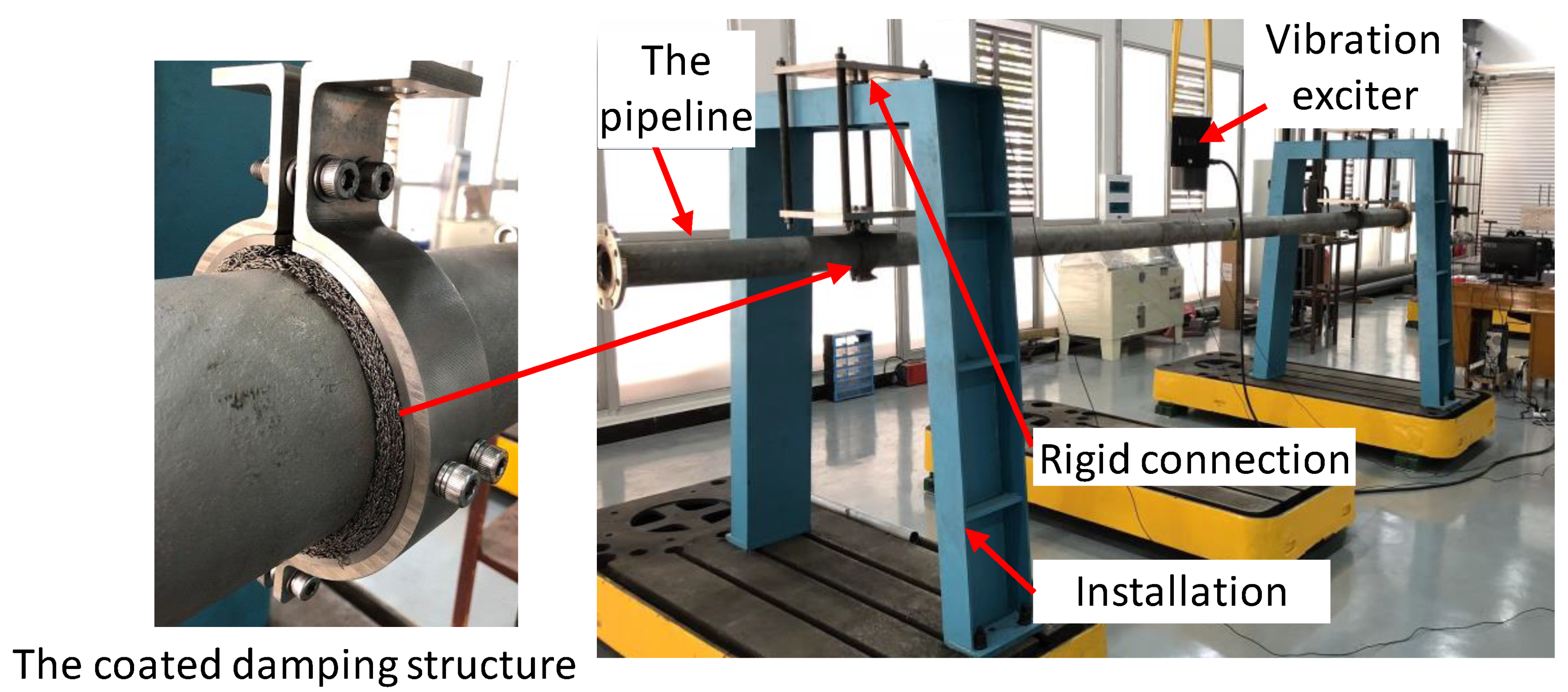
4. Experimental Verification

In this section, the reliability of the dynamic model presented in Section 3 is considered to be verified by the physical experiment. The main section context includes the introduction of the experiment equipment, dynamic testing methods and result analysis for the two-point and symmetrically pipeline system.

4.1. Case Description

To further explore the nonlinear dynamic model proposed in this paper, according to the installation method of engineering application, the experimental bench of the coated pipeline system as shown in Figure 3 was established. The experimental system mainly contained the following five parts: The excitation system, data acquisition system and measurement system; the pipeline with two-point and symmetrically supported brackets; the coated damping structure; the installation base; and the rigid connection. The excitation system consists of JZK-50 vibration exciter (maximum excitation force 500 N, amplitude ±10 mm) and E5874A power amplifier. The data acquisition system consists of VT-900X vibration controller with data acquisition and analysis software. The measurement system consists of YD-303 piezoelectric quartz force sensor and KD9004 eddy current displacement senor. The coated damping structure was composed of elastic-porous metal rubber, coated rings, and the specific coated form. The related experiment equipment and effective test method can be found in the previous works [27]. It should be pointed out that the coated damping structure with elastic-porous metal rubber has a sound effect on vibration reduction of the pipeline system [28]. In this work, the application of elastic-porous metal rubber for the damping element enwrapped on the outer wall of the pipeline was due to its excellent vibration absorption performance [29,30].

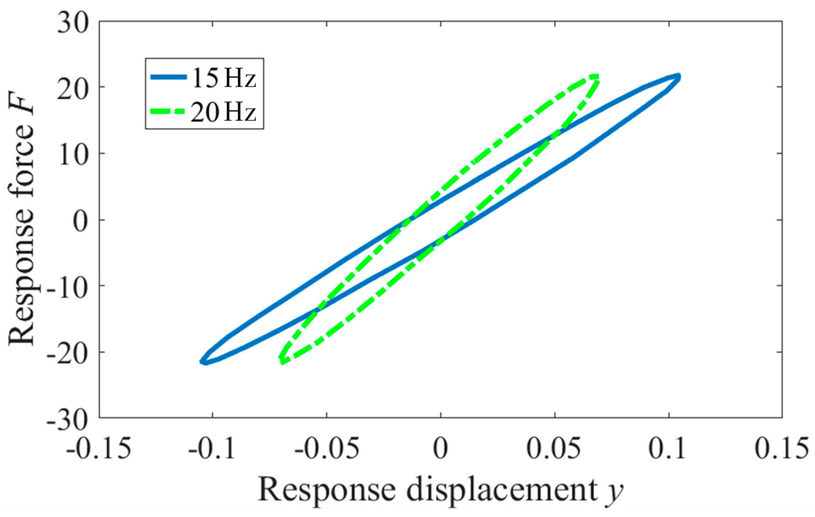
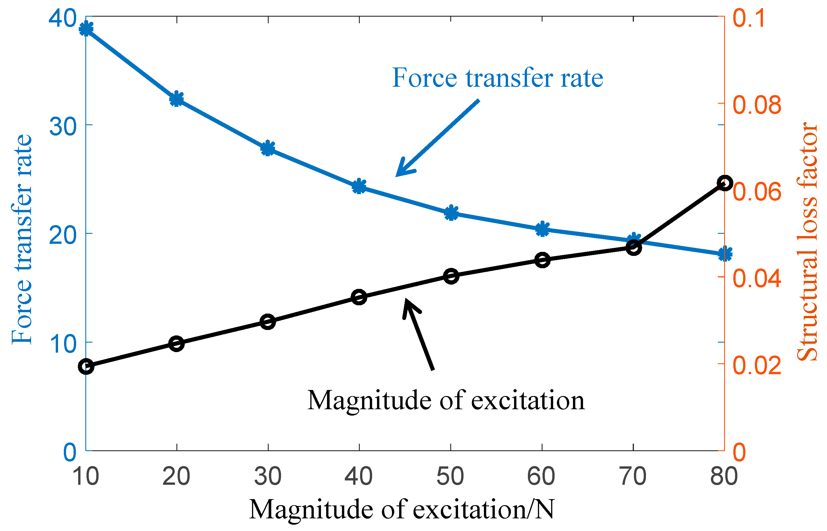
4.2. Nonlinearity and Energy Consumption

During the experimental test, the sinusoidal excitation force with various frequencies was applied to the coated pipeline system and its displacement response was measured. For the unification of excitation magnitude, an excitation condition of 40 mvpp for the pipeline system with the voltage loading amplitude was adopted. The curve of response force F and response displacement y can be plotted as Figure 4 when the excitation frequencies of 15 Hz and 20 Hz were used respectively.

It can be observed from Figure 4 that the coated pipeline system has an obvious nonlinearity. This can mainly be caused by the used elastic-porous metal rubber in the system as a nonlinear damping structure with energy dissipation characteristics. It should be mentioned that the total restoring force of elastic-porous metal rubber coated damped structure is composed of nonlinear elastic restoring force and nonlinear damping force. Nonlinear elastic restoring force denoted by an inclined curve in Figure 4 plays a restoring role in the working process of elastic-porous metal rubber, and nonlinear damping force mainly dissipates the damping energy. The measured dynamic results show a good accordance with the analytical expression of Equation (49). In Equation (49), z(t) as a nonlinear component of elastic-porous metal rubber has a hysteresis characteristic. In the view of physical mechanism based on material microstructure, z(t) is associated with the slip force and slip displacement produced by the dynamic movement between the coiled wires, which possesses both stiffness and damping.

According to the dynamic parameter identification of loss factor η, energy dissipation ∆W and maximum elastic potential energy W in [30,31], the energy dissipation characteristics of the corresponding coated pipeline system under 15 Hz and 20 Hz experimental conditions are obtained, as listed in

Table 1. The energy dissipation characteristics of the coated pipeline system.

Frequency (Hz)	Energy Dissipation ΔW (N·mm)	Maximum Elastic Potential Energy W (N·mm)	Loss Factor η
15	1.016	1.136	0.142
20	0.822	0.752	0.174

.

Table 1 indicates that a reduction existing in the energy dissipation ∆W with the increase of frequency. This phenomenon can be explained by the displacement of the coated damping structure decreases with the excitation frequency increases under a constant excitation force. From the microscopic level, with the decrease of displacement, the slip distance between metal wires in metal rubber is reduced, and the capacity for energy dissipation of elastic-porous metal rubber becomes weaker. Meanwhile, it is known that the maximum elastic potential energy is proportional to displacement, and the maximum elastic potential energy of elastic-porous metal rubber may degrade with the reduction of displacement. The loss factor in Table 1 represents the ratio of the energy dissipation to the maximum elastic potential energy. The maximum elastic potential energy shows a faster speed of degradation than the energy dissipation, which leads to an augmentation of loss factor.

The experimental dynamic results associated with the energy dissipation characteristics would be nonlinear in terms of the change of frequency. This is attributed to the resonance frequency of the coated pipeline system. Thus, the dynamic test with the sinusoidal sweep frequency should be considered in the following work. It should be noted that one limitation of the conducted research is that it is difficult to accurately identify dynamic properties of the used coating damping structure. This is due to the damping element, namely elastic-porous metal rubber, which exhibits obvious nonlinear characteristics and has not been determined very well so far.

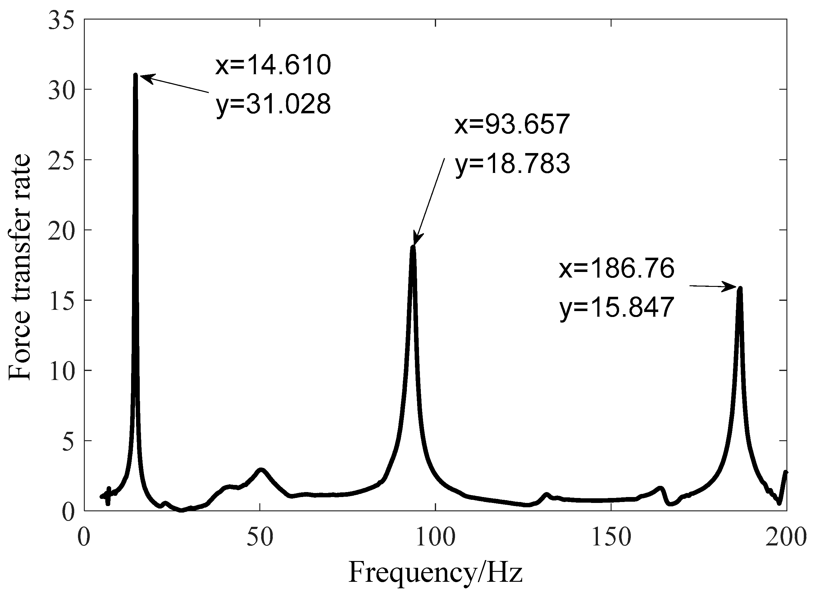
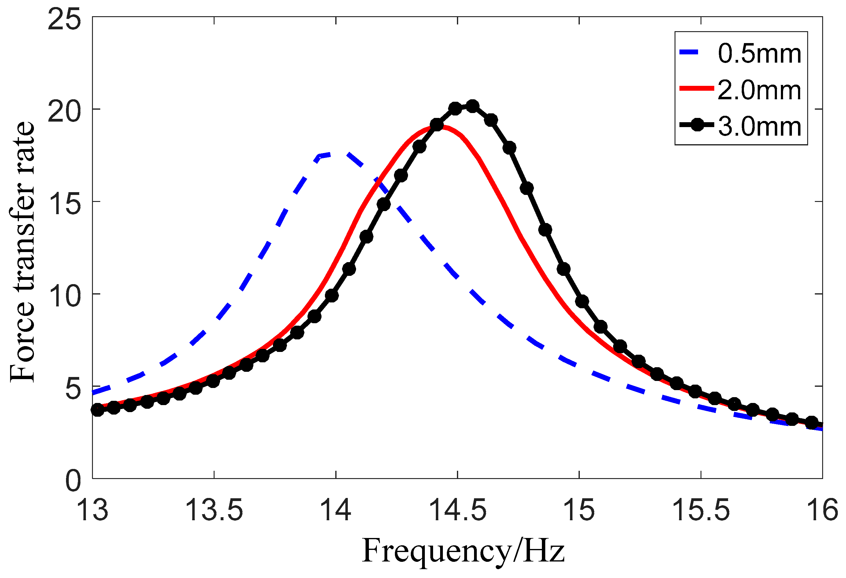
4.3. Dynamic Test and Its Result

The dynamic test with a broadband sweep frequency range (5–200 Hz) for the coated pipeline system was performed to improve the reliability of the experiment. Two layers of elastic-porous metal rubber were used, and the magnitude of excitation applied is set as 20 N. The experimentally measured force transfer rate-frequency curve can be plotted as Figure 5. It can be seen that the system exists three modes in the frequency range of 5–200 Hz. They are 14.610 Hz, 93.657 Hz, 186.76 Hz, respectively. The corresponding response force F and the response displacement y are not consistent under the conditions of 15 Hz and 20 Hz as mentioned in the Section 4.2. Due to the condition of 15 Hz as the resonance frequency band, the response force of the whole system is far greater than the basic force. This is reasonable for the dynamic analysis. Due to the increase of the response displacement caused by the resonance, the displacement under 15 Hz is larger than other frequencies. However, when the excitation frequency is up to 20 Hz, the non-resonant station of the coated pipeline system occurs, resulting in the degradation of the response force and the corresponding response displacement.

Figure 6 shows that the peak of the force transfer rate T_Am decreases gradually and the structural loss factor η linearly increases with the increase of the magnitude of the excitation. This is due to that the vibration damping amplitude of the elastic-porous metal rubber increases with the increase of excitation magnitude. The slip amplitude between the inner metal wires increases, leading to the increase of energy dissipation. The energy dissipation of elastic-porous metal rubber is generated by the sliding dry friction between the inner hooked wires. When the excitation magnitude increases from 10 N to 80 N, the force transfer rate obviously decreases and the loss factor shows an obvious increase trend. The excitation magnitude plays a considerable role on the energy dissipation of elastic-porous metal rubber and its vibration damping system.

Integrated with the excitation magnitude of 80 N, different pre-tightening conditions (0.5 mm, 2 mm, 3 mm) were applied to the coated pipeline system. Figure 7 shows the corresponding force transfer rate curves. The peak of the force transfer rate T_Am can be obtained and then the structural loss factor η is calculated based on the half-power method, as listed in

Table 2. Energy dissipation characteristics at different pre-tightening conditions.

Energy Dissipation Characteristics	Pre-Tightening Conditions (mm)
	0.5	2	3
Natural Frequency ωn (Hz)	13.996	14.420	14.538
Peak of the Force Transfer Rate TAm	17.682	19.025	20.182
Structural Loss Factor η	0.0533	0.0454	0.0435

.

As can be seen from Figure 7 and Table 2, the variation of pre-tightening conditions not only affects the natural frequency of the system, but also affects the energy dissipation characteristics of the coated pipeline system. The natural frequency increases with the increase of pre-tightening. The peak T_Am of the force transfer rate increases, the structural loss factor η decreases, and the energy dissipation characteristics degrades. The source of this phenomenon may be that with the increase of pre-tightening, the contact pairs between metal wires are obviously dense and the slipping movements between wires become relatively difficult. When the excitation condition is always 80 N, the slip amplitude is relatively slight under the condition of large pre-tightening with the same exciting magnitude. Additionally, the slip amplitude decreases with the increase of pre-tightening.

5. Conclusions

In this paper, a dynamic analysis based on impulse response matrix to describe two-point and symmetrically supported pipeline bracket system was performed by means of mathematically modelling. The dynamic model involved of rigid pipeline, nonlinear elastic connection structure and coated damping structure is simplified and established. As for the experimental verification, the sinusoidal sweep dynamic tests were carried out to obtain the first three modes of the coated pipeline damping system and compared with the analytical results. The experimental response force-displacement curves and the energy dissipation characteristics under different excitation conditions were obtained to analyse the nonlinear characteristics of the coated pipeline system. The dynamic experimental results show a good agreement with the developed dynamic model. This work should be of great significance for the dynamic analysis of pipeline system with a damping structure. The obtained dynamic model should be further explored and validated by means of more application cases with different boundary configurations. For example, two-point and symmetrically supported pipeline bracket systems with different damping elements or different service environments.

References

1. Li, Y.D.; Yang, Y.R. Vibration analysis of conveying fluid pipe via He’s variational iteration method. Appl. Math. Model. 2016, 43, 409–420. [Google Scholar]
2. Zhou, K.; Xiong, F.R.; Jiang, N.B.; Dai, H.L.; Yan, H.; Wang, L.; Ni, Q. Nonlinear vibration control of a cantilevered fluid-conveying pipe using the idea of nonlinear energy sink. Nonlinear Dyn. 2019, 95, 1435–1456. [Google Scholar] [CrossRef]
3. Zhang, T.; Qu, Y.H.; Zhang, Y.O.; Lv, B.L. Nonlinear dynamics of straight fluid-conveying pipes with general boundary conditions and additional springs and masses. Appl. Math. Model. 2016, 40, 7880–7900. [Google Scholar] [CrossRef]
4. Bao, R. Efficient dynamics analysis of large-deformation flexible beams by using the absolute nodal coordinate transfer matrix method. Multibody Syst. Dyn. 2014, 32, 535–549. [Google Scholar]
5. Lin, W.; Qiao, N. Nonlinear dynamics of a fluid-conveying curved pipe subjected to motion-limiting constraints and a harmonic excitation. J. Fluids Struct. 2008, 24, 96–110. [Google Scholar] [CrossRef]
6. Zhang, Z.W.; Wang, Y.J.; Wang, W.; Tian, Y.L. Periodic Solution of the Strongly Nonlinear Asymmetry System with the Dynamic Frequency Method. Symmetry 2019, 11, 676. [Google Scholar] [CrossRef] [Green Version]
7. Meng, D.; Guo, H.Y.; Xu, S.P. Non-linear dynamic model of a fluid-conveying pipe undergoing overall motions. Appl. Math. Model. 2011, 35, 781–796. [Google Scholar] [CrossRef]
8. Yu, D.L.; Wen, J.H.; Zhao, H.G. Vibration reduction by using the idea of phononic crystals in a pipe-conveying fluid. J. Sound Vib. 2008, 318, 193–205. [Google Scholar] [CrossRef]
9. Bi, K.M.; Hao, H. Using pipe-in-pipe systems for subsea pipeline vibration control. Eng. Struct. 2016, 109, 75–84. [Google Scholar] [CrossRef] [Green Version]
10. Modarres-Sadeghi, Y.; Paıdoussis, M.P. Nonlinear dynamics of extensible fluid-conveying pipes, supported at both ends. J. Fluids Struct. 2009, 25, 535–543. [Google Scholar] [CrossRef]
11. Amabili, M. Nonlinear damping in large-amplitude vibrations: Modelling and experiments. Nonlinear Dyn. 2018, 93, 5–18. [Google Scholar] [CrossRef]
12. Kong, X.R.; Li, H.Q.; Wu, C. Dynamics of 1-dof and 2-dof energy sink with geometrically nonlinear damping: Application to vibration suppression. Nonlinear Dyn. 2018, 91, 733–754. [Google Scholar] [CrossRef]
13. Rezaiee-Pajand, M.; Sarafrazi, S.R. Nonlinear dynamic structural analysis using dynamic relaxation with zero damping. Eng. Struct. 2011, 89, 1274–1285. [Google Scholar] [CrossRef]
14. Zhai, J.; Li, J.; Wei, D.; Gao, P.; Yan, Y.; Han, Q. Vibration control of an aero pipeline system with active constraint layer damping treatment. Appl. Sci. 2019, 9, 2094. [Google Scholar] [CrossRef] [Green Version]
15. Dong, G.X.; Zhang, Y.H.; Luo, Y.J.; Xie, S.; Zhang, X.N. Enhanced isolation performance of a high-static-low-dynamic stiffness isolator with geometric nonlinear damping. Nonlinear Dyn. 2018, 93, 2339–2356. [Google Scholar] [CrossRef]
16. Gao, K.; Gao, W.; Wu, D. Nonlinear dynamic stability analysis of Euler-Bernoulli beam-columns with damping effects under thermal environment. Nonlinear Dyn. 2017, 90, 2423–2444. [Google Scholar] [CrossRef]
17. Wang, G.P.; Rong, B.; Tao, L.; Rui, X.T. Riccati discrete time transfer matrix method for dynamic modeling and simulation of an underwater towed system. J. Appl. Mech. 2012, 79, 041014. [Google Scholar] [CrossRef]
18. Rong, B.; Lu, K.; Rui, X.T.; Li, X.J.; Tao, L.; Wang, G.P. Nonlinear dynamics analysis of pipe conveying fluid by Riccati absolute nodal coordinate transfer matrix method. Nonlinear Dyn. 2018, 92, 699–708. [Google Scholar] [CrossRef]
19. Rezaiee-Pajand, M.; Sarafrazi, S.R.; Rezaiee, H. Efficiency of dynamic relaxation methods in nonlinear analysis of truss and frame structures. Comput. Struct. 2012, 112, 295–310. [Google Scholar] [CrossRef]
20. Yang, P.; Bai, H.B.; Xue, X.; Xiao, K.; Zhao, X. Vibration reliability characterization and damping capability of annular periodic metal rubber in the non-molding direction. Mech. Syst. Signal Process. 2019, 132, 622–639. [Google Scholar] [CrossRef]
21. Chandrasekhar, K.; Rongong, J.; Cross, E. Mechanical behaviour of tangled metal wire devices. Mech. Syst. Signal Process. 2019, 118, 13–29. [Google Scholar] [CrossRef] [Green Version]
22. Zhang, D.Y.; Fabrizio, S.; Ma, Y.H. Dynamic mechanical behavior of nickel-based superalloy metal rubber. Mater. Des. 2014, 56, 69–77. [Google Scholar] [CrossRef]
23. Wang, H.; Rongong, J.A.; Tomlinson, G.R. Nonlinear static and dynamic properties of metal rubber dampers. Int. Conf. Noise Vib. Eng. 2010, 10, 1301–1316. [Google Scholar]
24. Wu, K.N.; Bai, H.B.; Xue, X.; Li, T.; Li, M. Energy dissipation characteristics and dynamic modeling of the coated damping structure for metal rubber of bellows. Metals 2018, 8, 562. [Google Scholar] [CrossRef] [Green Version]
25. Ma, Y.H.; Zhang, Q.C.; Zhang, D.Y.; Scarpa, F.; Liu, B.L.; Hong, J. A novel smart rotor support with shape memory alloy metal rubber for high temperatures and variable amplitude vibrations. Smart Mater. Struct. 2014, 23, 125016. [Google Scholar] [CrossRef]
26. Kwon, S.C.; Jo, M.S.; Oh, H.U. Experimental Validation of Fly-Wheel Passive Launch and On-Orbit Vibration Isolation System by Using a Superelastic SMA Mesh Washer Isolator. Int. J. Aerosp. Eng. 2017, 2017, 1–16. [Google Scholar] [CrossRef] [Green Version]
27. Xiao, K.; Bai, H.B.; Xue, X.; Wu, Y.W. Damping characteristics of metal rubber in the pipeline coating system. Shock. Vib. 2018, 42, 1–11. [Google Scholar] [CrossRef] [Green Version]
28. Ma, Y.H.; Zhang, Q.C.; Zhang, D.Y.; Scarpa, F.; Gao, D.; Hong, J. Size-dependent mechanical behavior and boundary layer effects in entangled metallic wire material systems. J. Mater. Sci. 2017, 52, 3741–3756. [Google Scholar] [CrossRef] [Green Version]
29. Catania, G.; Strozzi, M. Damping oriented design of thin-walled mechanical components by means of multi-layer coating technology. Coatings 2018, 8, 73. [Google Scholar] [CrossRef] [Green Version]
30. Hou, J.F.; Bai, H.B.; Li, D.W. Damping capacity measurement of elastic porous wire-mesh material in wide temperature range. J. Mater. Process. Technol. 2008, 206, 412–418. [Google Scholar] [CrossRef]
31. Zhang, D.Y.; Fabrizio, S.; Ma, Y.H.; Boba, K.; Hong, J.; Lu, H.W. Compression mechanics of nickel-based superalloy metal rubber. Mater. Sci. Eng. A 2013, 580, 305–312. [Google Scholar] [CrossRef]
Figure 1. Physical model of vibration isolation system for the two-point and symmetrically supported pipeline bracket.
Symmetry 11 01479 g001
Figure 2. The coordinate of pipeline B.
Symmetry 11 01479 g002
Figure 3. The experimental bench of coated pipeline system.
Symmetry 11 01479 g003
Figure 4. The response curves of displacement and force.
Symmetry 11 01479 g004
Figure 5. The experimental measured force transfer rate-frequency curves of coated pipeline damping system.
Symmetry 11 01479 g005
Figure 6. The evolution of force transfer rate and loss factor with excitation level.
Symmetry 11 01479 g006
Figure 7. The force transfer rate-frequency curves.
Symmetry 11 01479 g007