Feature Selection Based on Swallow Swarm Optimization for Fuzzy Classification

Abstract

This paper concerns several important topics of the Symmetry journal, namely, pattern recognition, computer-aided design, diversity and similarity. We also take advantage of the symmetric structure of a membership function. Searching for the (sub) optimal subset of features is an NP-hard problem. In this paper, a binary swallow swarm optimization (BSSO) algorithm for feature selection is proposed. To solve the classification problem, we use a fuzzy rule-based classifier. To evaluate the feature selection performance of our method, BSSO is compared to induction without feature selection and some similar algorithms on well-known benchmark datasets. Experimental results show the promising behavior of the proposed method in the optimal selection of features.

1. Introduction and Literature Review

Feature selection implies extracting a subset of features from an initial set, with these features being fully relevant to a problem at hand or the training problem. Feature selection makes it possible to (1) avoid overfitting, (2) reduce the amount of data to be analyzed, (3) improve the accuracy of classification, (4) eliminate irrelevant and "noisy" features, (5) improve the interpretability of results, and (6) visualize data [1,2].

An increase in the number of features causes a decrease in the performance of training algorithms, which contradicts the intuitive notion that a larger number of features provides more information and improves the accuracy of classification. The reason is that, with increasing number of features, it is also necessary to increase the amount of training data, which are required to generate classification rules. These rules determine the relationship between features and class labels. In addition, features that do not contain information about class labels can reduce classification accuracy and slow down the training process [3]

Feature selection methods are divided into three groups: filters, wrappers, and embedded methods [4,5,6]. Filters are based on the generalized properties of training data and do not use any classifier construction algorithm in the process of feature selection. The advantages of this approach are relatively low computational complexity, sufficient generalization capability, and independence from the classifier. Its main disadvantage is that features are often selected independently [6]. Wrappers include the classifier construction procedure in the feature selection process and use the prognostic accuracy of the classifier to estimate the selected subset of features. The interaction with the classifier generally yields better results as compared to filters; however, it increases the computational complexity of the method and there is a risk of overfitting [6]. Embedded methods select features in the process of training and integrate the feature selection procedure into the classifier construction algorithm. In [7], a hybrid method that combines filters, wrappers, and feature weighting was proposed.

In [6], it was noted that there is no best method for feature selection, and the researcher should focus on finding a good method for each particular problem.

The feature selection problem can be modeled as a binary optimization problem [8], which is an NP-hard one [4]. Its optimal solution is guaranteed only by exhaustive search. Metaheuristic methods allow one to find sub-optimal solutions of this problem without exploring the entire solution space. However, most metaheuristics were designed for a continuous search space. A binary search space poses the problem of discontinuity and non-differentiability, which makes it difficult to use classical deterministic optimization methods [9]. In binary problems, it is required to reduce the number of possible states to binary solutions. There are many binarization methods; below, we discuss the main ones.

In this paper, we present a novel method for feature selection based on binary swallow swarm optimization (BSSO). The binarization of the continuous swallow swarm metaheuristics is carried out using a special function.

The main contribution of this paper is as follows.

• The original swallow swarm algorithm is designed for continuous optimization; for the first time we offer a new binary version of swallow swarm optimization for solving binary optimization problems.
• A novel feature selection method based on binary swallow swarm optimization is proposed. This is the first work applying the binary swallow swarm optimization to feature selection.
• As an example of building fuzzy rule-based classifiers, the proposed method is compared with wrapper feature selections based on other metaheuristics, feature selection algorithm based on mutual information, and algorithm without feature selection.
• The Wilcoxon signed-rank test is used to evaluate the proposed method.
• A multiple regression equation is found that reflects the relationship between the BSSO runtime and the number of features, the number of instances, and the number of classes.

The paper is organized as follows. Section 1 overviews some related works. In Section 2, a fuzzy rule-based classifier is presented. Section 3 describes an algorithm for generating the fuzzy rule base. Feature selection based on the proposed method is discussed in Section 4. In Section 5, the experimental setups and results are presented. Finally, Section 6 provides the conclusions.

1.1. Literature Review

In this section, we discuss some works related to our research, which address the binarization of the metaheuristics designed for continuous optimization.

The genetic algorithm (GA) is one of the well-known tools for binary optimization and feature selection. GA solutions are represented as a set of binary vectors over which selection, crossover, and mutation are performed [10,11,12,13].

Harmonic search uses a special type of memory that stores harmonic solutions. A harmonic is a vector of binary values. In [14], we investigated two methods for forming a new harmonic: By inverting the current bit and by replacing the current bit with the bit of the best harmonic available in the harmonic memory. Both the methods were used in the fuzzy classifier for feature selection. In [15], harmonic search was employed to select features from multidimensional unbalanced datasets.

The ant colony optimization algorithm [16] was proposed for solving combinatorial optimization problems. This algorithm is also employed for feature selection: In [17], for a Takagi-Sugeno fuzzy classifier; in [18], for a classifier based on a back propagation neural network; in [19], for C4.5, naive Bayes, and k-nearest neighbor classifiers; and in [20], for support vector machine, linear discriminant analysis, random forest, k-nearest neighbors, and decision tree classifiers.

However, most metaheuristics were designed for searching in a continuous space; hence, to solve binary optimization problems, they need to be modified. Below, we describe the most popular methods used to binarize continuous metaheuristics without affecting the principles of the search process.

1.1.1. Quantum Methods

In [21], the problems of feature selection and parameter optimization for neural networks were solved using a quantum particle swarm optimization (PSO) method, with features being represented as quantum bits (Q-bits). The principles of quantum superposition and quantum probability were employed to speed up the search for the optimal set of features.

Researchers in [22] proposed a hybrid swarm intelligence algorithm based on quantum computations and a combination of the firefly algorithm and PSO for feature selection. Quantum computations provided a good tradeoff between the intensification and diversification of search, while the combination of the firefly algorithm and PSO made it possible to efficiently investigate the generated subsets of features. To evaluate the relevance of these subsets, rough set theory was employed.

Han and Kim in [23] described a quantum evolutionary algorithm based on the concept and principles of quantum computing. The algorithm represents a solution as a Q-bit chromosome and uses a quantum operator to update it (this operator is a modified version of the logical rotation operator).

In [24], to solve binary optimization problems, a quantum gravitational search algorithm was designed by supplementing the basic structure of the gravitational search procedure with the following elements of quantum computing: quantum bit, quantum measurements, superposition, and modified quantum rotation operators.

1.1.2. Modified Algebraic Operations

Yuan et al. in [25] described the binary PSO algorithm; it has all basic characteristics of the classical PSO with the only difference being a zero inertia coefficient. To evaluate the velocity of particles, subtraction was replaced by the XOR operator, arithmetic multiplication was replaced by conjunction (AND), and addition was replaced by disjunction (OR). To compute a new position of the particle, addition was replaced by the XOR operator. The same logical operators were employed in [26] to discretize the swallow swarm optimization algorithm when solving the traveling salesman problem.

In [27], four logical operators—OR, AND, XOR and NOT—were analyzed as applied to the binarization of the artificial bee colony algorithm and only two of them (XOR and NOT) were found useful.

Korkmaz and Kiran [28] modified the artificial algae algorithm to solve the binary optimization problem. The modification involved the introduction of the XOR operator and the stigmergic update rule. Stigmergic behavior was implemented using two new counters affected by the results of the XOR operator and artificial agents in the algorithm.

In [29], binarization of the continuous spider monkey algorithm was performed using the logical operators AND, OR, and XOR. The proposed algorithm is designed for thinning of concentric circular antenna arrays. In [30], the binary spider monkey algorithm is used to feature selection for a fuzzy classifier.

In the binary artificial bee colony algorithm called DisABC [31], the arithmetic difference operator in the continuous algorithm was replaced by the measure of difference between binary vectors, expressed in terms of Jaccard’s coefficient. A specific property of this measure is that, even in a continuous space, its result can be used to generate a new binary solution vector. To improve the efficiency of DisABC, it was supplemented with a local search procedure. This procedure changes the value of the zero bit in the binary vector to 1 while simultaneously setting the bit with the value 1 to 0. The procedure does not change the number of 1-valued bits in the vector [31].

1.1.3. Transfer Functions

In binary metaheuristics, transfer functions are responsible for transforming the continuous search space into the discrete one. In 1997, Kennedy and Eberhart were the first to apply a sigmoid transfer function in the binary version of PSO [32]. In [33], six transfer functions divided into two families—S-shaped and V-shaped—were used for the binarization of PSO. The comparative analysis showed that the family of V-shaped transfer functions significantly improves the performance of the binary PSO.

The widespread use of transfer functions is hindered by the lack of a methodology for selecting these functions as a good alternative to simple trial and error. This selection can be dynamic, taking into account past search experience [34]. In [35], to achieve a tradeoff between the diversification and intensification of PSO, time-varying transfer functions were proposed.

In the binary version of gravitational search [36], some basic concepts associated with updating the positions of particles were modified. The current value of bits was changed with the probability computed based on the velocity of a particle, i.e., the binary gravitational search algorithm updated the velocity and formed a new position of the particle as 1 or 0 with the given probability. In [34], it was suggested that, for slow velocities, the probability of change in the position of a particle should be close to zero, while for fast velocities, this probability should be high. As a probability function, the hyperbolic tangent was employed. In [37], binary gravitational search with S-shaped and V-shaped functions was used to select features for a fuzzy classifier; in [38], for a classifier based on k-nearest neighbors.

S-shaped and V-shaped transfer functions were successfully applied to binarize the butterfly optimization algorithm [39], the grasshopper optimization algorithm [40], dragonfly algorithm [41], the gray wolf algorithm [42], the salp swarm algorithm [43], and the brainstorm algorithm [44]; they were also used to construct hybrid binary algorithms [45].

In [46], an algorithm based on k-means clustering was proposed for the binarization of continuous swarm intelligence metaheuristics. The authors also presented a methodology for setting binarization parameters, which allows one to control the binarization process.

2. Fuzzy Rule-Based Classifier

Fuzzy classifiers, which belong to rule-based methods, have significant advantages in terms of their functionality, as well as their design and subsequent analysis. A unique advantage of fuzzy classifiers is the interpretability of classification rules [47,48].

Suppose that x = (x₁, x₂, …, x_D)∈R^D is a D-dimensional feature space and C = {c₁, c₂, …, c_m} is a set of class labels. Then, the classification problem can be reduced to defining, on the set of class labels, a label that corresponds to the feature vector of an object to be classified.

A fuzzy classifier is given by a base of production rules of the following form [37]:

R_i: IF s₁∧x₁ = A_1i AND s₂∧x₂ = A_2i AND … AND s_D∧x_D = A_Di THEN class = c_i, i = 1, …, R,

where A_ki is the fuzzy term that characterizes the k-th feature in the i-th fuzzy rule (k = 1,…, D), R is the number of fuzzy rules, and S = (s₁, s₂, …, s_D) is the binary feature vector, where s_k∧x_k indicates the presence (s_k = 1) or absence (s_k = 0) of a feature in the classifier.

On a given dataset {(x_p; c_p), p = 1, 2, …, Z} the class label is defined as follows:

$$\begin{array}{l}class=c_t,t=\arg \underset{j=1,2,\dots ,m}{\max }{\beta }_j,\\ {\beta }_j\left(x_p\right)={\displaystyle \sum _{\begin{array}{c}{R}_i\\ clas{s}_i=c_j\end{array}}{\displaystyle \prod _{k=1}^D{\mu }_{A_{ki}}(x_{pk})}},\end{array}$$

${\mu }_{A_{ki}}(x_{pk})$ is the symmetric membership function for the fuzzy term A_ki at the point x_pk.

The measure of classification rate is defined as a ratio between the number of correctly assigned class labels and the total number of objects to be classified:

$$E(\theta ,S)=\frac{{\displaystyle \sum _{p=1}^Z\{\begin{array}{l}1,if{c}_p=\arg \underset{j=1,2,\dots ,m}{\max }{f}_j\left(x_p;\theta ,S\right)\\ 0,otherwise\end{array}}}{Z},$$

(1)

where f(x_p; θ, S) is the output of the fuzzy classifier with the parameters θ and features S at the point x_p.

To construct the fuzzy classifier, two problems—fuzzy rule base generation and feature selection—need to be solved. The first problem is solved by generating a fuzzy rule base based on the extreme values in each class, while the second problem is solved by the BSSO algorithm.

3. Fuzzy Rule Base Generation

The algorithm generates the initial rule base for the fuzzy classifier that contains one rule of each class [49]. The rules are formed based on the extreme values in the training sample T_r = {(x_p; c_p), p = 1, 2,…, Z}. Let us introduce the following designations: m is the number of classes; D is the number of features. A pseudo code of the Fuzzy rule base generation algorithm is shown in Algorithm 1.

Algorithm 1 Fuzzy rule base generation algorithm.

1: Input: m, Tr. 2: Output: fuzzy rule base Ri (where i = 1, 2…, m). 3: begin 4: for i←1 to m do 5:  for k←1 to D do 6:    $\mathrm{Search}\mathrm{a}\mathrm{left}\mathrm{border}\mathrm{of}\mathrm{membership}\mathrm{function}{\mu }_{A_{ki}}\left(x_k\right)$:     7:                     $a\leftarrow \underset{(p=1,2,\dots ,Z)\wedge (c_p=i)}{\min }{x}_{pk}$; 8: $\mathrm{Search}\mathrm{a}\mathrm{right}\mathrm{border}\mathrm{of}\mathrm{membership}\mathrm{function}{\mu }_{A_{ki}}\left(x_k\right)$: 9:                     $c\leftarrow \underset{(p=1,2,\dots ,Z)\wedge (c_p=i)}{\max }{x}_{pk}$; 10: Calculate a center of $\mathrm{membership}\mathrm{function}{\mu }_{A_{ki}}\left(x_k\right)$: 11:                     b ← a + (c – a)/2; 12: Create a symmetric triangular membership function with borders a and c, and center b for fuzzy term Aki; 13: end 14: $\mathrm{Create}\mathrm{rule}{R}_i\mathrm{with}{\mu }_{A_{ki}}\left(x_k\right)$ membership functions (where k = 1, 2, …, D) and output ck ← k; 15: end 16: end

4. Wrapper-Based Feature Selection Algorithm

4.1. Swallow Swarm Optimization

Swallow swarm optimization is a population-based metaheuristic based on the algorithm proposed in 2013 by Neshat et al. for a continuous case [50].

At the beginning of each iteration, the population is sorted based on the value of the objective function. Then, the following roles are assigned:

• Head leader is a particle with the best value of the objective function;
• Local leaders are l particles that follow the head leader in accordance with the value of the objective function;
• Aimless particles are k particles with the worst value of the objective function;
• Explorers are all other particles.

On the current iteration, head leaders do not move, acting as beacons for explorer particles, which, in turn, explore the search space between the nearest local leader and the head leader. Explorer particles change their positions by the following formulas:

$$\begin{array}{l}{\mathsf{\theta }}_e\left(t+1\right)={\mathsf{\theta }}_e\left(t\right)+V\left(t+1\right),\\ V\left(t+1\right)=VHL\left(t+1\right)+VLL\left(t+1\right),\\ VHL\left(t+1\right)=VHL\left(t\right)+rand\left(0,1\right)\left({\mathsf{\theta }}_e^{best}\left(t\right)-{\mathsf{\theta }}_e\left(t\right)\right)+rand\left(0,1\right)\left({\mathsf{\theta }}_{HL}\left(t\right)-{\mathsf{\theta }}_e\left(t\right)\right),\\ VLL\left(t+1\right)=VLL\left(t\right)+rand\left(0,1\right)\left({\mathsf{\theta }}_e^{best}\left(t\right)-{\mathsf{\theta }}_e\left(t\right)\right)+rand\left(0,1\right)\left({\mathsf{\theta }}_{LL}\left(t\right)-{\mathsf{\theta }}_e\left(t\right)\right),\end{array}$$

where θ_e is the position of the explorer, θ_HL is the position of the head leader, θ_LL is the position of the local leader nearest to the explorer, θ_e^best is the best position, $V$ is the velocity vector of the particle, $VHL$ is the velocity vector of the particle moving to the head leader, and $VLL$ is the velocity vector of the particle moving to the nearest local leader.

In contrast to [50] we decide not to select the parameters α_HL, β_HL,

α_LL and β_LL which are used to compute the velocity vectors with respect to the head and local leaders. Our experiments showed that the corresponding procedure increases the runtime of the algorithm without any significant improvement of the result. In this work, all these parameters are set to 1.

The formula for changing the positions of aimless particles is also modified because the original formula can cause particles to gather at the boundaries of the search space or even go beyond it. Our formula reduces the probability of this behavior and also allows explorer particles to slightly affect the behavior of aimless particles. To change the position of aimless particles, the following formulas are used:

$$\begin{array}{l}{\mathsf{\theta }}_O\left(t+1\right)=rand(0.5,2)\cdot V\mathbf{S}\mathbf{S},\\ V\mathbf{S}\mathbf{S}=\frac{{\displaystyle \sum _{j=1}^{N-k}{\mathsf{\theta }}_e^j\left(t\right)}}{N-k},\end{array}$$

where θ_O is the position of aimless particle, θ^j is the position of the j-th particle, N is the total number of particles in the population, and k is the number of aimless particles.

Once the termination condition is met, the algorithm returns the position of the head leader as a new solution.

4.2. Binary Swallow Swarm Optimization Algorithm

This section describes the proposed feature selection method based on the binary swallow swarm optimization (BSSO) algorithm. BSSO adapts the original algorithm to solve feature selection problems.

In [26], the authors provide discrete swallow swarm optimization to solve the well-known traveling salesman problem. This algorithm uses operators that can only be used to solve this particular problem. Here, the position is a Hamiltonian cycle, and the velocity is defined as a set of permutation between two cities. In contrast to [26] in this work, we use a special function merge to update the position of particles. As its input, this function receives two vectors X and Y, as well as the number p, which determines the influence of X on Y, ranging from 0 to 1. The function merge yields the vector Z each element of which is found as follows: if the values X_i and Y_i coincide, then has the same value; otherwise, Z_i takes the value X_i with the probability p or takes the value Y_i with the probability (1–p).

$$merge{\left(X,Y,p\right)}_i=\{\begin{array}{l}{X}_i,ifrand\left(0,1\right)<p\\ Y_i,otherwise\end{array},i=1,2,\dots ,D.$$

This is due to the fact that all solutions have different classification accuracies. If a feature is included in a solution that has higher classification accuracy, then this feature is more likely to be relevant. Conversely, if a feature is not included in a solution with higher classification accuracy, then this feature is more likely to be noise. Thus, this approach allows a new solution to include more features that are potentially relevant and to exclude more features that are potentially noise. On the other hand, by varying p, it is possible to control the effect of randomness when computing a new solution, so that the algorithm does not converge too quickly and is not stuck at local optima.

This algorithm represents solutions as vectors S that encode features. At the first step of the algorithm, a population (set) of vectors S is generated (randomly or in some other way). The number of vectors in the population is a preset integer, which is also referred to as the population size. For each vector, a measure of classification accuracy E is computed (Equation (1)). On each iteration, all vectors are sorted in descending order of E. The first element becomes the head leader. The next l solutions are local leaders, n worst vectors are aimless particles, and all other vectors are explorer particles. The integer variables l and n are also specified beforehand. Explorer particles change their positions based on the positions of the leaders, while aimless particles do so randomly.

Below are the corresponding formulas for explorers:

$$\begin{array}{l}{S}_e\left(t+1\right)=merge\left(V\left(t+1\right),S_e\left(t\right),p_{ve}\right),\\ V\left(t+1\right)=merge\left(VHL\left(t+1\right), VLL\left(t+1\right),p_{vhl}\right),\\ VHL\left(t+1\right)=merge\left(merge\left(SHL\left(t\right),S_e\left(t\right),p_{he}\right),rand{\left\{0,1\right\}}^D, p_{her}\right),\\ VLL\left(t+1\right)=merge\left(merge\left(SLL\left(t\right),S_e\left(t\right),p_{le}\right),rand{\left\{0,1\right\}}^D,p_{ler}\right),\end{array}$$

(2)

where SHL is the position of the head leader, SLL is the position of the local leader, S_e is the position of the explorer, VHL is the velocity vector with respect to the head leader, VLL is the velocity vector with respect to the nearest local leader, V is the common velocity vector, p_ve is the effect of the velocity vector on the position of the explorer, p_vhl is the effect of the velocity vector with respect to the head leader on the velocity vector with respect to the local leader, p_he is the effect of the head leader’s position on the position of the explorer, p_her is the combined effect of the head leader and explorer on a random vector, p_le is the effect of the local leader’s position on the position of the explorer, and p_ler is the combined effect of the local leader and explorer on a random vector. A pseudo code of the BSSO is shown in Algorithm 2.

Algorithm 2 Binary Swallow Swarm Optimization.

1: Input: train data. 2: Output: SHL – position of the head leader. 3: Parameters: iterations – maximum number of cycles, N – population size, D – dimension, pvs, pvhl, phe, pher, ple, pler, l – local leaders, k – aimless particles. 4: begin 5: for i ← to N do 6:   Initialize each solution Si in the population: Si ← rand{0,1}D; 7:    Select j-th (j = 1,2,…,D) feature for subset Sub where Sij = 1; 8:   Build reduced dataset (subtra) based on Sub; 9:   Evaluate fitness value (fitnessi) of Sub: fitnessi ← errorrate;     Evaluate fitness value (fitnessi) of Sub: fitnessi ← errorrate; 10: end 11:  SHL ← Sk, where $k=\underset{i=1,2,..,N}{\min }\left(fitnes{s}_i\right)$; 12: for iter←1 to iterations do 13:    for i ← to N do 14:       Find nearest local leader SLL among population {S1, S2, …, SN}; 15:       Evolve a new solution Se={f1, f2, …, fD} using Equation (2); 16:       Select j-th feature (j = 1,2,…,D) for subset Sub, where Sej = 1; 17:       Build reduced dataset (subtra) based on Sub; 18:        Evaluate fitness value (fitnessi) of Sub: fitnessi ← errorrate; 19:       if fitnessSe< fitnessi then 20:          Si ← Se; 21:          fitnessi ← fitnessSe; 22:       end 23:    end 24:     $\mathbf{SHL}\leftarrow {\mathbf{S}}^k,\mathrm{where}k=\underset{i=1,2,..,N}{\min }\left(fitnes{s}_i\right)$; 25: end 26: end

5. Experiment

5.1. Datasets and Parameter Setting

To validate our method, we used 30 real datasets from the knowledge extraction based on evolutionary learning (KEEL) repository [51]. The experiment was carried out as follows: first, a fuzzy classifier was constructed on all features from the source dataset. Then, using the feature selection algorithm, some of the features were removed, and the classification accuracy on the remaining features was estimated. Parameter optimization was not carried out. The experiments were conducted based on the tenfold cross-validation scheme, whereby the optimal subset of features was determined on each of ten subsamples. The fuzzy classifier was constructed on the subset found, and its average classification accuracy was determined on the training and test datasets. At the end of the experiment, the average number of selected features and the average accuracy of classification based only on these features were determined.

Table 1. Distributions of datasets.

Dataset	Number of Classes	Number of Features	Number of Examples
apendicitis	2	7	106
balance	3	4	625
banana	2	2	5300
bupa	2	6	345
cleveland	5	13	297
coil2000	2	85	9822
contraceptive	3	9	1473
dermatology	6	34	358
ecoli	8	7	336
glass	7	9	214
haberman	2	3	306
heart	2	13	270
hepatitis	2	19	80
ionosphere	2	33	351
iris	3	4	150
magic	2	10	19020
newthyroid	3	5	215
optdigits	10	64	5620
ring	2	20	7400
segment	7	19	2310
spambase	2	57	4597
tae	3	5	151
texture	11	40	5500
thyroid	3	21	7200
titanic	2	3	2201
twonorm	2	20	7400
vehicle	4	18	846
wdbc	2	30	569
wine	3	13	178
wisconsin	2	9	683

describes 30 datasets used in the experiments.

The parameter settings for the BSSO algorithm are shown in

Table 2. Parameter settings for BSSO.

Parameter	Setting
N—Population of particles	40
l—local leaders	3
k—aimless particles	6
Iterations	300
pve	0.7
pvhl	0.7
phe	0.9
pher	0.9
ple	0.8
pler	0.8

.

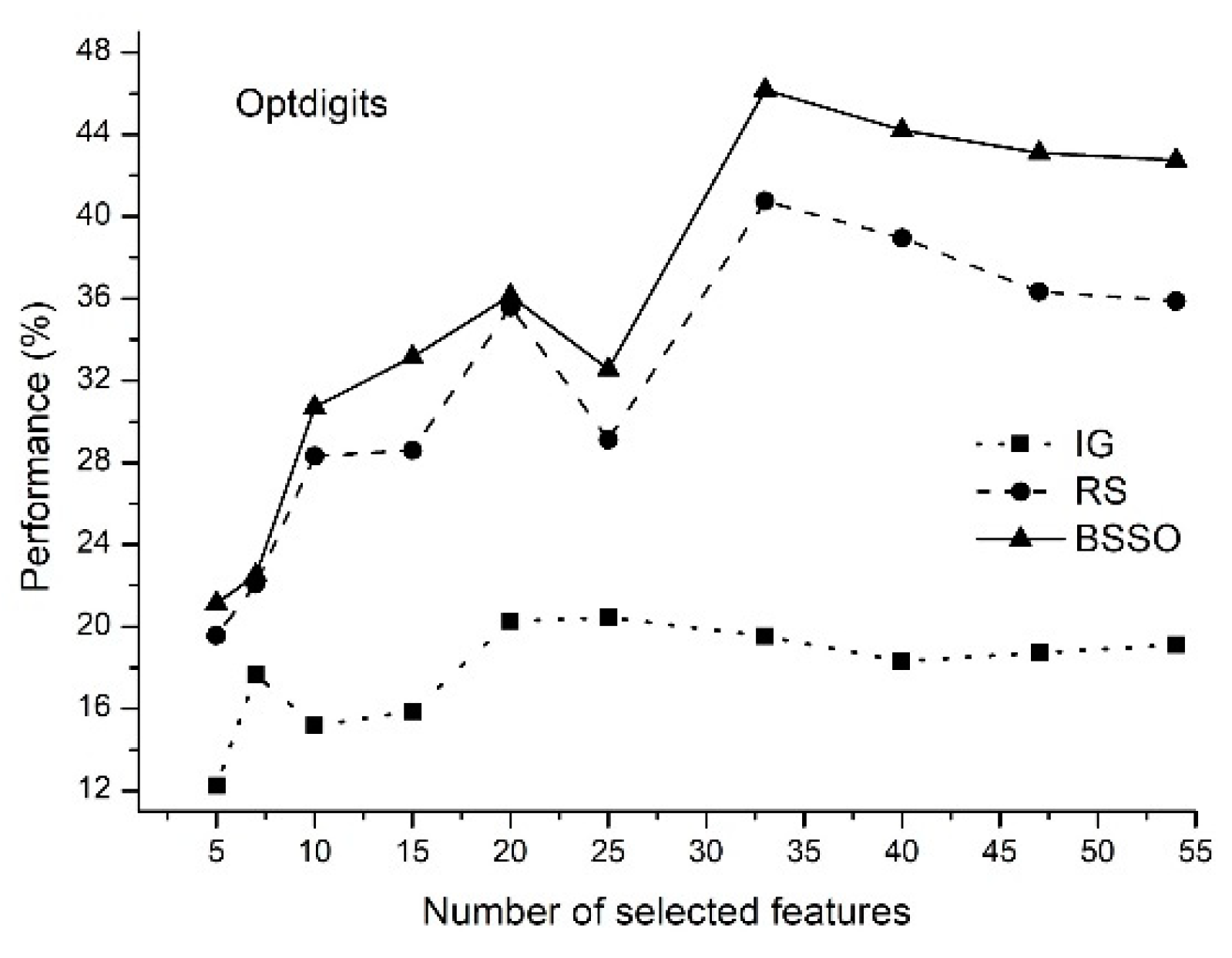
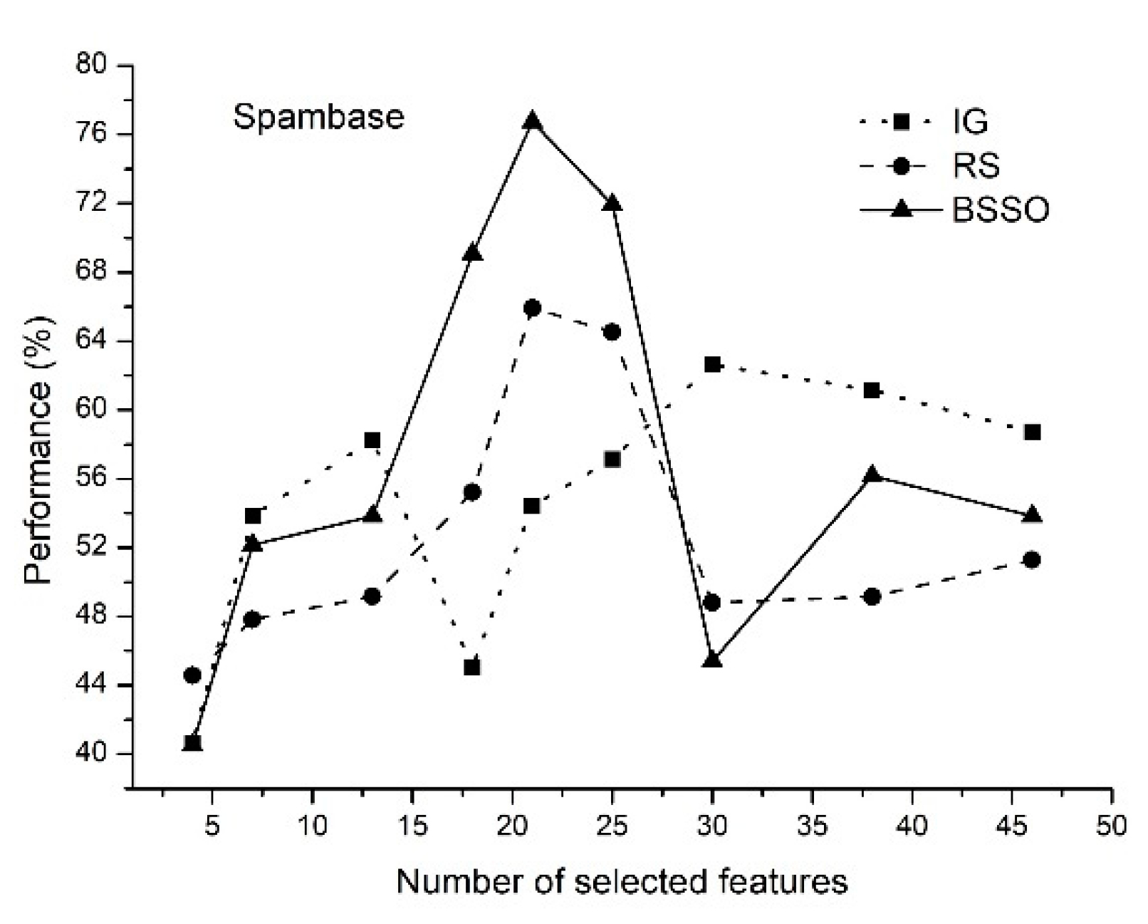
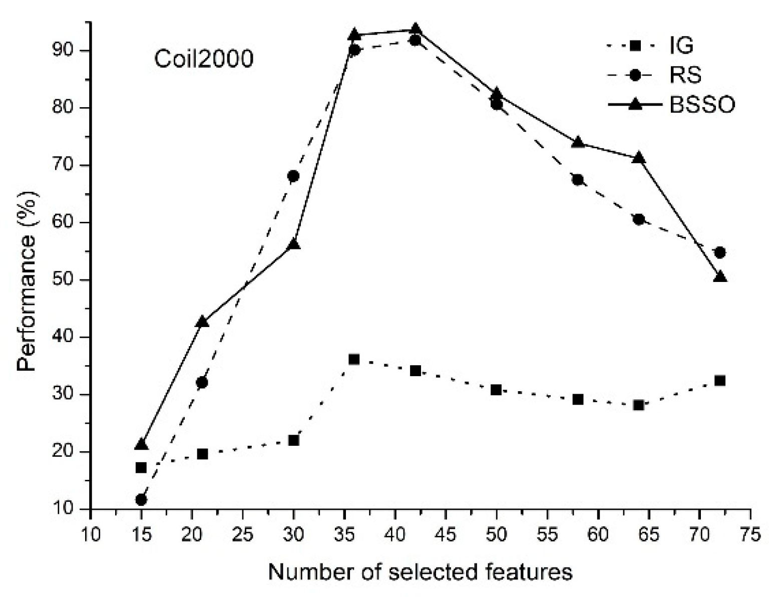
5.2. Comparison with the Other Approaches

BSSO was compared with two other representative methods, wrapper feature selection based on a random search algorithm (RS), feature selection algorithm based on mutual information (IG), and algorithm without feature selection (All features) on 30 benchmark datasets.

BSSO was compared with other representative methods, wrapper feature selections based on the binary spider monkey algorithm (BSMA) [30], the binary gravitational search algorithm (BSGA) [37], the binary brain storm optimization algorithm (BBSO) [52], the random search algorithm (RS), as well as a feature selection algorithm based on mutual information (IG) [53], and a algorithm without feature selection (All features) on well-known benchmark datasets.

Then, the averaged error rates were used as fitness values of the corresponding feature subsets. Equation (1) evaluates the best feature subset by using the fuzzy classifier without optimizing the classifier’s parameters to obtain the classification error rate.

For each dataset, experiments to examine the feature selection performance of each algorithm were conducted for 30 independent runs

Table 3. Accuracy comparison of the feature selection methods.

Dataset	All features		IG			BSSO			RS
	Learn	Test	F‘	Learn	Test	F‘	Learn	Test	F‘	Learn	Test
apendicitis	72.15	66.77	4.90	79.05	78.40	3.30	83.03	79.32	3.40	83.03	80.23
balance	46.24	46.25	2.00	38.88	38.90	3.60	46.26	45.93	3.50	46.26	45.77
banana	44.45	44.41	1.00	59.42	59.40	1.00	59.42	59.40	1.00	59.42	59.40
bupa	49.47	46.92	1.70	46.60	46.89	2.90	60.48	61.15	2.90	60.48	59.98
cleveland	54.07	54.04	5.00	53.58	53.05	7.70	57.02	51.63	7.20	56.95	51.28
coil2000	9.75	9.67	33.70	37.91	37.99	37.60	93.84	93.75	39.60	92.87	92.74
contraceptive	42.63	42.71	5.40	42.33	42.30	2.20	44.65	44.54	2.30	44.65	44.47
dermatology	93.95	89.68	13.00	41.14	38.09	20.80	97.73	92.46	19.20	97.30	92.46
ecoli	32.79	32.89	3.50	50.49	51.40	3.90	53.57	53.32	3.90	53.57	53.32
glass	55.81	52.65	3.30	25.31	21.62	6.00	61.00	54.02	6.30	63.54	52.71
haberman	45.43	45.47	2.00	44.73	44.83	1.10	70.15	70.61	1.10	70.15	70.61
heart	56.87	55.93	5.10	58.26	55.92	3.60	70.41	64.07	3.50	70.04	64.07
hepatitis	64.36	60.08	9.20	51.14	41.65	8.10	94.31	85.16	8.10	93.20	84.98
ionosphere	87.94	87.45	9.40	67.14	67.00	7.00	85.41	81.28	8.90	78.92	74.36
iris	93.85	94.00	2.00	96.74	96.67	2.10	96.89	94.67	2.00	96.89	94.67
magic	56.70	56.75	6.00	60.15	60.16	3.90	71.39	71.44	3.90	71.39	71.44
newthyroid	96.54	95.39	3.00	94.89	94.39	3.40	97.88	95.84	3.50	97.88	95.37
optdigits	23.41	23.12	22.30	24.46	24.10	37.80	47.32	46.00	35.60	42.93	41.72
ring	49.51	49.52	10.20	49.17	49.19	1.00	58.50	58.44	4.60	54.52	53.20
segment	72.20	71.48	6.00	20.31	20.09	8.30	88.26	86.02	8.80	87.78	85.46
spambase	56.81	56.73	27.90	63.84	64.29	22.60	73.57	73.45	25.10	70.93	70.74
tae	35.17	36.41	3.50	34.66	34.41	2.80	41.80	41.07	3.00	41.80	40.40
texture	64.48	68.55	19.10	27.88	27.84	13.00	68.49	68.31	16.00	66.85	66.09
thyroid	22.50	22.50	17.30	92.31	92.36	1.50	93.33	93.24	1.80	88.38	89.14
titanic	68.53	66.52	1.00	77.61	77.87	1.50	77.61	77.87	1.50	77.61	77.87
twonorm	96.87	96.91	10.10	88.32	88.20	19.70	96.89	96.91	19.90	96.67	95.68
vehicle	25.40	24.83	8.00	21.93	21.75	8.10	49.24	43.74	7.70	47.47	45.88
wdbc	90.43	90.17	18.50	93.40	92.97	10.90	97.34	96.12	11.70	96.09	95.78
wine	89.82	87.57	6.10	50.01	45.36	6.50	96.57	94.41	7.00	95.86	94.31
wisconsin	92.81	92.25	6.30	75.68	74.98	5.60	94.42	93.85	7.10	94.63	92.75
Average	59.70	58.92	8.88	55.58	54.74	8.58	74.23	72.27	9.00	73.27	71.23

shows the experimental results of four different feature selection methods. For each method, the table presents the average classification accuracy on the training set (Learn), the average classification accuracy on the test sample (Test), and the average number of the selected features (F‘).

Table 4. Results of using wrapper feature selection methods.

Dataset	BMA		BGA(S)		BGA(V)		BBA(S)		BBA(V)
	Test	F‘	Test	F‘	Test	F‘	Test	F‘	Test	F‘
apendicitis	76.36	2.90	Nr 1	nr	nr	nr	78.76	3.10	77.11	3.40
balance	46.24	4.00	nr	nr	nr	nr	46.08	3.04	46.08	3.04
banana	59.36	1.00	nr	nr	nr	nr	nr	nr	nr	nr
bupa	58.17	2.70	59.80	2.80	60.00	2.70	57.30	2.74	56.56	2.66
cleveland	54.15	8.20	52.50	7.30	54.40	2.80	53.30	6.40	52.00	8.36
coil2000	74.96	31.3	90.60	38.5	94.00	1.00	nr	nr	nr	nr
contraceptive	44.06	2.80	nr	nr	nr	nr	nr	nr	nr	nr
dermatology	90.99	21.6	nr	nr	nr	nr	nr	nr	nr	nr
ecoli	51.22	3.90	nr	nr	nr	nr	50.30	3.34	50.90	3.48
glass	56.12	6.20	56.00	5.10	53.20	5.90	57.60	5.30	55.40	5.73
haberman	67.96	1.10	nr	nr	nr	nr	57.50	1.90	57.60	1.90
heart	74.21	5.40	67.00	2.80	67.70	3.00	66.60	3.36	66.70	4.20
hepatitis	85.51	8.10	87.20	7.90	82.50	5.30	84.52	9.40	81.22	9.17
ionosphere	91.58	16.8	nr	nr	nr	nr	89.29	16.4	89.81	18.2
iris	94.67	1.80	nr	nr	nr	nr	95.07	1.92	94.80	1.90
magic	nr	nr	70.70	4.10	70.70	4.10	71.41	3.90	70.41	4.32
newthyroid	96.77	3.50	96.50	3.70	96.50	3.30	93.67	4.15	94.02	4.20
optdigits	nr	nr	nr	nr	nr	nr	nr	nr	nr	nr
ring	58.39	1.00	58.60	1.00	57.90	1.00	nr	nr	nr	nr
segment	81.90	9.00	85.70	9.10	84.10	8.80	nr	nr	nr	nr
spambase	74.27	23.7	65.40	27.0	70.00	2.70	nr	nr	nr	nr
tae	nr	nr	nr	nr	nr	nr	nr	nr	nr	nr
texture	73.69	12.1	nr	nr	nr	nr	nr	nr	nr	nr
thyroid	90.93	1.80	99.30	20.0	99.30	16.9	nr	nr	nr	nr
titanic	77.60	1.40	nr	nr	nr	nr	nr	nr	nr	nr
twonorm	96.74	19.7	96.80	19.9	96.10	17.8	nr	nr	nr	nr
vehicle	47.87	5.90	45.60	7.80	40.00	4.80	43.05	6.16	40.55	6.56
wdbc	95.18	10.4	nr	nr	nr	nr	nr	nr	nr	nr
wine	96.08	6.20	94.80	5.80	92.20	6.80	92.39	6.28	93.56	6.74
wisconsin	93.59	5.30	94.00	5.70	93.60	3.50	nr	nr	nr	nr

¹ nr—no report.

shows the average of accuracy and number of features for wrapper methods, here the symbol S means the use of the S-shaped transfer function, and the symbol V means the use of the V-shaped function.

A statistical significance test (related-samples Wilcoxon signed-rank test) was carried out to assess the classification performance of the methods. The test is considered “safer” because it does not imply normal distribution, and outliers have less effect on the result [12]. The purpose of the Wilcoxon test is to determine whether the results yielded by two methods are independent (i.e., reject the null hypothesis). The null hypothesis was that different feature selection methods generate similar results or the median of differences between different feature selection methods equals zero. The null hypothesis is rejected (the p-value is less than or equal to the significance level) if the differences between the methods are significant. The significance level in the Wilcoxon test is selected as 0.05. Table 4 shows the results of the Wilcoxon test for the pairwise comparison of BSSO and different feature selection methods and algorithm without feature selection. The BCCO algorithm showed better accuracy and fewer features compared to the RS algorithm. These differences are statistically significant. The BCCO algorithm showed better accuracy and fewer features compared to the IG algorithm. Differences in accuracy are statistically significant. Differences in the number of characters are not statistically significant. The BCCO algorithm showed better accuracy and fewer features (with the exception of two cases) compared to other metaheuristics, although these differences are not statistically significant.

The feature selection is a binary optimization problem, and the No Free Lunch theorem assumes that no concrete algorithm gives the best results for all optimization problems [54], so new optimization algorithms are being developed. It was noted in [6] that there is no single best method for feature selection, and the researcher should focus on finding a good method for each specific problem.

The time taken to execute the proposed BSSO is given in

Table 5. Paired two-tailed Wilcoxon test between BSSO and the other methods with significance level 0.05.

Median of Differences	Standardized Test Statistic	p-Value	Null Hypothesis
BSSO_Learn—All_Learn	4.659	<0.001	Reject
BSSO_Learn—IG_Learn	4.623	<0.001	Reject
BSSO_Learn—RS_Learn	3.070	0.002	Reject
BSSO_Test—All_Test	4.206	<0.000	Reject
BSSO_Test—IG_Test	4.418	<0.000	Reject
BSSO_Test—RS_Test	3.263	0.001	Reject
BSSO_Test—BSMA_Test	0.127	0.899	Retain
BSSO_Test—BGSA(S)_Test	−0.379	0.879	Retain
BSSO_Test—BGSA(V)_Test	1.060	0.299	Retain
BSSO_Test—BBSO(S)_Test	0.682	0.496	Retain
BSSO_Test—BBSO(V)_Test	1.363	0.173	Retain
BSSO_F‘—IG_F‘	−0.389	0.697	Retain
BSSO_F‘—RS_F‘	−2.027	0.043	Reject
BSSO_F‘—BSMA_F‘	−0.522	0.602	Retain
BSSO_F‘—BGSA(S)_F‘	−0.455	0.649	Retain
BSSO_F‘—BGSA(V)_F‘	1.847	0.065	Retain
BSSO_F‘—BBSO(S) _F	−0.502	0.615	Retain
BSSO_F‘—BBSO(V) _F	−1.193	0.233	Retain

in comparison with the time required for execution of IG and RS. All these methods were executed on the same machine with configurations: Intel Core i5-3570, with 3.40 GHz and a RAM of 8 GB. #C has been used as the programming language.

As can be seen from

Table 6. Execution time (seconds).

Dataset	BSSO	RS	IG
apendicitis	2.4969	1.7509	0.0690
balance	8.6825	7.2545	0.0909
banana	28.8653	26.7955	0.1769
bupa	4.3853	4.0395	0.0807
cleveland	13.7823	10.5905	0.1189
coil2000	649.0763	502.0300	115.3146
contraceptive	25.6143	23.5633	0.2409
dermatology	34.5858	30.0775	0.2775
ecoli	12.4913	12.1631	0.1179
glass	7.7928	7.5788	0.1019
haberman	2.7073	2.3386	0.0730
heart	5.3957	3.7275	0.0929
hepatitis	2.5654	2.1653	0.0760
ionosphere	11.6846	11.0012	0.1689
iris	2.2396	2.0328	0.0700
magic	210.2207	186.0533	6.4670
newthyroid	3.9593	3.8287	0.0780
optdigits	1355.8079	1300.9188	26.0010
ring	135.9984	75.0970	2.5237
segment	134.1489	124.1207	1.0419
spambase	213.8056	145.8274	11.2431
tae	2.4275	2.4025	0.0710
texture	980.7259	679.4120	12.0827
thyroid	200.5548	113.6152	4.5406
titanic	10.3387	9.7130	0.1179
twonorm	200.8571	141.2837	4.1145
vehicle	29.2830	26.9224	0.2696
wdbc	16.3909	14.0634	0.2389
wine	4.9080	4.8560	0.0879
wisconsin	8.6997	8.2846	0.1189

, IG achieved the best execution time, mainly due to its structure, in which the classifier is missing. The binary SSO produced comparable results with RS. However, BSSO’s good accuracy on finding optimal solutions more than RS and IG compensates its computational inefficiency.

Based on the results of the experiment, the authors developed a relationship between execution time and number of attributes, number of instances, and number of classes using multiple linear regression. Regression finds the target function fitting the input data with minimum error. The regression equation is as follows:

tBSSO = -285.890 + 60.487∙NoCl +7.682∙NoFe + 0.022∙NoEx,

where tBSSO is the execution time of BSSO, NoCl is the number of classes, NoFe is the number of features, NoEx is the number of examples.

In our example, the fitted model has a coefficient of determination of R² = 0.782, which indicates that the model describes the data well. The

Table 7. Coefficients and their estimates.

Model	Unstandardized Coefficients		t		Sig. Level		95.0% Confidence Interval for B
	B	Std. Error					Lower Bound	Upper Bound
	(Constant)	−285.890	54.884	−5.209		0.000	−398.707	−173.074
	NoCl	60.487	11.764	5.142		0.000	36.306	84.667
	NoFe	7.682	1.607	4.780		0.000	4.378	10.985
	NoEx	0.022	0.007	2.975		0.006	0.007	0.037

shows a list of the estimated coefficients of the multiple linear regression model with the significance level, t-statistics and confidence intervals.

For three data sets, Optdigits, Spambase, Coil2000, three algorithms for selecting features were running, IG, RS, BSSO, and the number of selected functions for each algorithm was recorded. Then a fuzzy classifier was applied without optimizing the parameters for each newly acquired data set containing only the selected functions. Figure 1, Figure 2 and Figure 3 shows the average classification rates of the methods in the testing partitions versus the number of selected features.

Figure 1, Figure 2 and Figure 3 shows that the suggested method exhibits the best performance. Based on the foregoing, we can draw the following conclusions.

• The proposed method of feature selection on some data sets allows to obtain a classification rate exceeding 90%, which indicates that the feature selection method is effective by reducing the amount of data processing.
• The classification rate of the increases with an increase in the number of features selected. When the number of selected features reaches a certain value, the classification rate decreases.
• The proposed method allows selecting the optimal features.

6. Conclusions

In this paper, we have addressed the problem of wrapper-based feature selection. We have applied binary swallow swarm optimization to the problem of feature selection for fuzzy classification. It is important to note that the parameters of the fuzzy classifier have not been optimized, and the number of fuzzy rules has been minimal (it corresponded to the number of classes in the dataset).

The proposed feature selection method is based on a special function that compares two binary vectors to form a new one, taking into account the effect of the first vector on the second one. This approach allows a new solution to include more features that are potentially relevant and to exclude more features that are potentially noise.

To demonstrate that the performance of BSSO is statistically significant in comparison to the other feature selection methods, the non-parametric Wilcoxon signed-ranks test with the significant level of 0.05 has been carried out. Based on the results of the investigation, it can be concluded that BSSO is competitive with the other methods.

BSSO has one disadvantage that we will address in our future work. This disadvantage is a large number of tunable parameters that need to be selected empirically. Transfer learning can be a solution to this problem. We also intend to investigate the effectiveness of the proposed method in constructing classifiers of other types.

Two disadvantages can be attributed to the BSSO. The first one is a large number of tunable parameters that need to be selected empirically. Transfer learning can be a solution to this problem. The second drawback of BSSO, which all wrappers have, is heavy computational burden. This disadvantage comes from the nature of this approach.

In the future, we also intend to investigate the effectiveness of BSSO in constructing classifiers of other types.

References

1. Garcia, S.; Luengo, J.; Herrera, F. Data Preprocessing in Data Mining; Intelligent Systems Reference Library; Springer International Publishing: Cham, Switzerland; New York, NJ, USA; Berlin, Germany, 2015; Volume 72, pp. 59–139. ISBN 978-3-319-10246-7. [Google Scholar]
2. Alkuhlani, A.; Nassef, M.; Farag, I. Multistage Feature Selection Approach for High-Dimensional Cancer Data. Soft Comput. 2017, 21, 6895–6906. [Google Scholar] [CrossRef]
3. Jalalirad, A.; Tjalkens, T. Using Feature-Based Models with Complexity Penalization for Selecting Features. J. Signal Process. Syst. 2018, 90, 201–210. [Google Scholar] [CrossRef]
4. Kohavi, R.; John, G.H. Wrappers for Feature Subset Selection. Artif. Intell. 1997, 97, 273–324. [Google Scholar] [CrossRef]
5. Ramirez-Gallego, S.; Mourino-Talin, H.; Martinez-Rego, D.; Bolon-Canedo, V.; Benitez, J.M.; Alonso-Betanzos, A.; Herrera, F. An Information Theory-Based Feature Selection Framework for Big Data Under Apache Spark. IEEE Trans. Syst. Man Cybern. Syst. 2018, 48, 1441–1453. [Google Scholar] [CrossRef]
6. Bolon-Canedo, V.; Sanchez-Marono, N.; Alonso-Betanzos, A. Feature Selection for High-Dimensional Data; Springer: Heidelberg, Germany, 2015; ISBN 978-3-319-21857-1. [Google Scholar]
7. Singh, D.; Singh, B. Hybridization of Feature Selection and Feature Weighting for High Dimensional Data. Appl. Intell. 2019, 49, 1580–1596. [Google Scholar] [CrossRef]
8. Hamedmoghadam, H.; Jalili, M.; Yu, X. An Opinion Formation Based Binary Optimization Approach for Feature Selection. Phys. A Stat. Mech. Its Appl. 2018, 491, 142–152. [Google Scholar] [CrossRef]
9. Banitalebi, A.; Aziz, M.I.A.; Aziz, Z.A. A Self-Adaptive Binary Differential Evolution Algorithm for Large Scale Binary Optimization Problems. Inf. Sci. 2016, 367, 487–511. [Google Scholar] [CrossRef]
10. Yang, J.; Honavar, V. Feature Subset Selection Using a Genetic Algorithm. IEEE Intell. Syst. 1998, 13, 44–49. [Google Scholar] [CrossRef]
11. Raymer, M.L.; Punch, W.F.; Goodman, E.D.; Kuhn, L.A.; Jain, A.K. Dimensionality Reduction Using Genetic Algorithms. IEEE Trans. Evol. Comput. 2000, 4, 164–171. [Google Scholar] [CrossRef]
12. Wu, K.; Yap, K. Feature Extraction; Guyon, I., Nikravesh, M., Gunn, S., Zadeh, L.A., Eds.; Studies in Fuzziness and Soft Computing; Springer: Berlin/Heidelberg, Germany, 2006; Volume 207, ISBN 978-3-540-35488-8. [Google Scholar]
13. Kabir, M.M.; Shahjahan, M.; Murase, K. A New Local Search Based Hybrid Genetic Algorithm for Feature Selection. Neurocomputing 2011, 74, 2914–2928. [Google Scholar] [CrossRef]
14. Hodashinsky, I.A.; Mekh, M.A. Fuzzy Classifier Design Using Harmonic Search Methods. Program. Comput. Softw. 2017, 43, 37–46. [Google Scholar] [CrossRef]
15. Moayedikia, A.; Ong, K.L.; Boo, Y.L.; Yeoh, W.G.; Jensen, R. Feature Selection for High Dimensional Imbalanced Class Data Using Harmony Search. Eng. Appl. Artif. Intell. 2017, 57, 38–49. [Google Scholar] [CrossRef]
16. Dorigo, M.; Maniezzo, V.; Colorni, A. The Ant System: Optimization by a Colony of Cooperating Agents. IEEE Trans. Syst. Man Cybern. Part B 1996, 26, 29–41. [Google Scholar] [CrossRef] [PubMed]
17. Vieira, S.M.; Sousa, J.M.C.; Runkler, T.A. Ant Colony Optimization Applied to Feature Selection in Fuzzy Classifiers. Lect. Notes Comput. Sci. 2007, 4529, 778–788. [Google Scholar]
18. Erguzel, T.T.; Ozekes, S.; Gultekin, S.; Tarhan, N. Ant Colony Optimization Based Feature Selection Method for QEEG Data Classification. Psychiatry Investig. 2014, 11, 243. [Google Scholar] [CrossRef] [PubMed]
19. Saraç, E.; Ozel, S.A. An Ant Colony Optimization Based Feature Selection for Web Page Classification. Sci. World J. 2014, 16, 649260. [Google Scholar] [CrossRef]
20. Ghimatgar, H.; Kazemi, K.; Helfroush, M.S.; Aarabi, A. An Improved Feature Selection Algorithm Based on Graph Clustering and Ant Colony Optimization. Knowl. Based Syst. 2018, 159, 270–285. [Google Scholar] [CrossRef]
21. Abdull Hamed, H.N.; Kasabov, N.K.; Shamsuddin, S.M. Quantum-Inspired Particle Swarm Optimization for Feature Selection and Parameter Optimization in Evolving Spiking Neural Networks for Classification Tasks. In Evolutionary Algorithms; InTech: Rijeka, Croatia, 2011; pp. 133–148. [Google Scholar]
22. Zouache, D.; Ben Abdelaziz, F. A Cooperative Swarm Intelligence Algorithm Based on Quantum-Inspired and Rough Sets for Feature Selection. Comput. Ind. Eng. 2018, 115, 26–36. [Google Scholar] [CrossRef]
23. Han, K.H.; Kim, J.H. Quantum-Inspired Evolutionary Algorithms with a New Termination Criterion, He Gate, and Two-Phase Scheme. IEEE Trans. Evol. Comput. 2004, 8, 164–171. [Google Scholar] [CrossRef]
24. Nezamabadi-Pour, H. A Quantum-Inspired Gravitational Search Algorithm for Binary Encoded Optimization Problems. Eng. Appl. Artif. Intell. 2015, 40, 62–75. [Google Scholar] [CrossRef]
25. Yuan, X.; Nie, H.; Su, A.; Wang, L.; Yuan, Y. An Improved Binary Particle Swarm Optimization for Unit Commitment Problem. Expert Syst. Appl. 2009, 36, 8049–8055. [Google Scholar] [CrossRef]
26. Bouzidi, S.; Riffi, M.E. Discrete Swallow Swarm Optimization Algorithm for Travelling Salesman Problem. In Proceedings of the ACM International Conference Proceeding Series, Rabat, Morocco, 21–23 July 2017; ACM Press: New York, NY, USA, 2017; Volume F1305, pp. 80–84. [Google Scholar]
27. Kiran, M.S.; Gunduz, M. XOR-Based Artificial Bee Colony Algorithm for Binary Optimization. Turk. J. Electr. Eng. Comput. Sci. 2013, 21, 2307–2328. [Google Scholar] [CrossRef]
28. Korkmaz, S.; Kiran, M.S. An Artificial Algae Algorithm with Stigmergic Behavior for Binary Optimization. Appl. Soft Comput. J. 2018, 64, 627–640. [Google Scholar] [CrossRef]
29. Singh, U.; Salgotra, R.; Rattan, M. A Novel Binary Spider Monkey Optimization Algorithm for Thinning of Concentric Circular Antenna Arrays. IETE J. Res. 2016, 62, 736–744. [Google Scholar] [CrossRef]
30. Hodashinsky, I.A.; Nemirovich-Danchenko, M.M.; Samsonov, S.S. Feature Selection for Fuzzy Classifier Using the Spider Monkey Algorithm. Bus. Inform. 2019, 13, 29–42. [Google Scholar] [CrossRef]
31. Kashan, M.H.; Nahavandi, N.; Kashan, A.H. DisABC: A new artificial bee colony algorithm for binary optimization. Appl. Soft Comput. J. 2012, 12, 342–352. [Google Scholar] [CrossRef]
32. Kennedy, J.; Eberhart, R.C. A Discrete Binary Version of the Particle Swarm Algorithm. In Proceedings of the 1997 IEEE International Conference on Systems, Man, and Cybernetics. Computational Cybernetics and Simulation, Orlando, FL, USA, 12–15 October 1997; IEEE: Piscataway, NJ, USA, 1997; Volume 5, pp. 4104–4108. [Google Scholar]
33. Mirjalili, S.; Lewis, A. S-Shaped Versus V-Shaped Transfer Functions for Binary Particle Swarm Optimization. Swarm Evol. Comput. 2013, 9, 1–14. [Google Scholar] [CrossRef]
34. Crawford, B.; Soto, R.; Astorga, G.; Garcia, J.; Castro, C.; Paredes, F. Putting Continuous Metaheuristics to Work in Binary Search Spaces. Complexity 2017, 2017, 8404231. [Google Scholar] [CrossRef]
35. Islam, M.J.; Li, X.; Mei, Y. A Time-Varying Transfer Function for Balancing the Exploration and Exploitation Ability of a Binary PSO. Appl. Soft Comput. J. 2017, 59, 182–196. [Google Scholar] [CrossRef]
36. Rashedi, E.; Nezamabadi-Pour, H.; Saryazdi, S. BGSA: Binary Gravitational Search Algorithm. Nat. Comput. 2010, 9, 727–745. [Google Scholar] [CrossRef]
37. Bardamova, M.; Konev, A.; Hodashinsky, I.; Shelupanov, A. A Fuzzy Classifier with Feature Selection Based on the Gravitational Search Algorithm. Symmetry 2018, 10, 609. [Google Scholar] [CrossRef]
38. Xiang, J.; Han, X.; Duan, F.; Qiang, Y.; Xiong, X.; Lan, Y.; Chai, H. A Novel Hybrid System for Feature Selection Based on an Improved Gravitational Search Algorithm and k-NN Method. Appl. Soft Comput. J. 2015, 31, 293–307. [Google Scholar] [CrossRef]
39. Arora, S.; Anand, P. Binary Butterfly Optimization Approaches for Feature Selection. Expert Syst. Appl. 2019, 116, 147–160. [Google Scholar] [CrossRef]
40. Mafarja, M.; Aljarah, I.; Faris, H.; Hammouri, A.I.; Al-Zoubi, A.M.; Mirjalili, S. Binary Grasshopper Optimisation Algorithm Approaches for Feature Selection Problems. Expert Syst. Appl. 2019, 117, 267–286. [Google Scholar] [CrossRef]
41. Mafarja, M.; Aljarah, I.; Heidari, A.A.; Faris, H.; Fournier-Viger, P.; Li, X.; Mirjalili, S. Binary Dragonfly Optimization for Feature Selection Using Time-Varying Transfer Functions. Knowl. Based Syst. 2018, 161, 185–204. [Google Scholar] [CrossRef]
42. Panwar, L.K.; Reddy, K.; Verma, A.; Panigrahi, B.K.; Kumar, R. Binary Grey Wolf Optimizer for Large Scale Unit Commitment Problem. Swarm Evol. Comput. 2018, 38, 251–266. [Google Scholar] [CrossRef]
43. Faris, H.; Mafarja, M.M.; Heidari, A.A.; Aljarah, I.; Al-Zoubi, A.M.; Mirjalili, S.; Fujita, H. An Efficient Binary Salp Swarm Algorithm with Crossover Scheme for Feature Selection Problems. Knowl. Based Syst. 2018, 154, 43–67. [Google Scholar] [CrossRef]
44. Papa, J.P.; Rosa, G.H.; De Souza, A.N.; Afonso, L.C.S. Feature Selection Through Binary Brain Storm Optimization. Comput. Electr. Eng. 2018, 72, 468–481. [Google Scholar] [CrossRef]
45. Mirjalili, S.; Wang, G.G.; Coelho, L.; Dos, S. Binary Optimization Using Hybrid Particle Swarm Optimization and Gravitational Search Algorithm. Neural Comput. Appl. 2014, 25, 1423–1435. [Google Scholar] [CrossRef]
46. Garcia, J.; Crawford, B.; Soto, R.; Astorga, G. A Clustering Algorithm Applied to the Binarization of Swarm Intelligence Continuous Metaheuristics. Swarm Evol. Comput. 2019, 44, 646–664. [Google Scholar] [CrossRef]
47. Hu, X.; Pedrycz, W.; Wang, X. Fuzzy Classifiers with Information Granules in Feature Space and Logic-Based Computing. Pattern Recognit. 2018, 80, 156–167. [Google Scholar] [CrossRef]
48. Ganesh Kumar, P.; Devaraj, D. Fuzzy Classifier Design Using Modified Genetic Algorithm. Int. J. Comput. Intell. Syst. 2010, 3, 334–342. [Google Scholar] [CrossRef]
49. Mekh, M.A.; Hodashinsky, I.A. Comparative Analysis of Differential Evolution Methods to Optimize Parameters of Fuzzy Classifiers. J. Comput. Syst. Sci. Int. 2017, 56, 616–626. [Google Scholar] [CrossRef]
50. Neshat, M.; Sepidnam, G.; Sargolzaei, M. Swallow Swarm Optimization Algorithm: A New Method to Optimization. Neural Comput. Appl. 2013, 23, 429–454. [Google Scholar] [CrossRef]
51. Alcala-Fdez, J.; Fernandez, A.; Luengo, J.; Derrac, J.; Garcia, S.; Sanchez, L.; Herrera, F. KEEL Data-Mining Software Tool: Data Set Repository, Integration of Algorithms and Experimental Analysis Framework. J. Mult. Log. Soft Comput. 2011, 17, 255–287. [Google Scholar]
52. Cheng, S. Brain Storm Optimization Algorithm, Concepts, Principles and Applications; Cheng, S., Shi, Y., Eds.; Springer: Cham, Switzerland, 2019; ISBN 978-3-030-15070-9. [Google Scholar]
53. Cai, J.; Luo, J.; Wang, S.; Yang, S. Feature Selection in Machine Learning: A New Perspective. Neurocomputing 2018, 300, 70–79. [Google Scholar] [CrossRef]
54. Wolpert, D.H. The Existence of a Priori Distinctions Between Learning Algorithms. Neural Comput. 1996, 8, 1341–1420. [Google Scholar] [CrossRef]
Figure 1. Dataset Optdigits. Average classification rates of the competing methods versus number of selected features.
Symmetry 11 01423 g001
Figure 2. Dataset Spambase. Average classification rates of the competing methods versus number of selected features.
Symmetry 11 01423 g002
Figure 3. Dataset Coil2000. Average classification rates of the competing methods versus number of selected features.
Symmetry 11 01423 g003