Dynamic Soft Sensor Development for Time-Varying and Multirate Data Processes Based on Discount and Weighted ARMA Models

Abstract

To solve the soft sensor modeling (SSMI) problem in a nonlinear chemical process with dynamic time variation and multi-rate data, this paper proposes a dynamic SSMI method based on an autoregressive moving average (ARMA) model of weighted process data with discount (DSSMI-AMWPDD) and optimization methods. For the sustained influence of auxiliary variable data on the dominant variables, the ARMA model structure is adopted. To reduce the complexity of the model, the dynamic weighting model is combined with the ARMA model. To address the weights of auxiliary variable data with different sampling frequencies, a calculation method for AMWPDD is proposed using assumptions that are suitable for most sequential chemical processes. The proposed method can obtain a discount factor value (DFV) of auxiliary variable data, realizing the dynamic fusion of chemical process data. Particle swarm optimization (PSO) is employed to optimize the soft sensor model parameters. To address the poor convergence problem of PSO, ω-dynamic PSO (ωDPSO) is used to improve the PSO convergence via the dynamic fluctuation of the inertia weight. A continuous stirred tank reactor (CSTR) simulation experiment was performed. The results show that the proposed DSSMI-AMWPDD method can effectively improve the SSM prediction accuracy for a nonlinear time-varying chemical process. The AMWPDD proposed in this paper can reflect the dynamic change of chemical process and improve the accuracy of SSM data prediction. The ω dynamic PSO method proposed in this paper has faster convergence speed and higher convergence accuracy, thus, these models correlate with the concept of symmetry.

1. Introduction

In order to reflect the dynamic change of chemical process, this paper attempts to propose DSSMI-AMWPDD method, which can effectively improve the prediction accuracy of nonlinear time-varying chemical process SSM. The proposed model and the concept of symmetry have relativity and complementarity, and the research direction is highly consistent with Symmetry, which is convenient for scholars in related fields as a reference. In chemical production, major process variables such as product quality are characterized by a slow sampling rate and time delay [1]. To ensure the stability of variable data in the main process, it is necessary to estimate the main process variables through some easily acquired process variables. Therefore, soft sensor modeling (SSMI) is of great significance. Since most chemical processes do not have clear principles but have strong nonlinear and dynamic time-varying characteristics, the use of data-driven methods to establish an industrial soft sensor model (SSM) [2,3,4] has become the focus of research. In particular, how to establish a suitable nonlinear dynamic model has evolved into an important research object for researchers.

Related modeling methods are generally divided into four types: multipoint input modeling [5,6,7], dynamic weighting modeling [8,9], feedback network modeling [10,11], and multimodel structure modeling [12,13,14]. Among these types of methods, multipoint input modeling boasts the advantages of simplicity, ease in implementation, and full reflection of the process characteristics. However, to fully reflect the dynamic characteristics of the process, a large number of high-dimensional input variables are needed, which increases the number and complexity of the internal parameters, resulting in ill-conditioned models. Dynamic weighting modeling uses dynamic weighting to form new input variables, which reduces the model input nodes and lower the model complexity, making the method simple and easy. However, the dynamic weights and historical data (HD) lengths are difficult to determine. Feedback network modeling updates the input through the delay link of the feedback loop and updates the structure or structural parameters, approximate to the object function. However, the model has poor stability, large deviations, no convergence, and an inability to fully reflect the dynamic information of the process; in addition, the model is not commonly used as it has a complex training process. A representative multimodel structure modeling is the Wiener structure, in which linear dynamic and nonlinear static submodels are built to describe the dynamic characteristics of a system. It provides a good approximation, but the dual model architecture is complex and difficult to identify.

The use of the above methods leads to inaccurate SSM data prediction, either because the sample data for modeling do not fully reflect the dynamic characteristics of the process or because it is difficult to perform the modeling and determine the parameters. To improve the prediction accuracy of SSM data and simplify the dynamic soft sensor modeling structure, this paper proposes an autoregressive moving average (ARMA) model of weighted process data with discount (AMWPDD) structure, which has better flexibility in actual time series data fitting [15] and is simple and easy to implement. Amid assumptions suitable for most sequential chemical processes, the discount factor (DF) is introduced for the auxiliary variable HD of a chemical process. Additionally, a DF calculation method and the corresponding constraints are proposed. Weighting is assigned to the auxiliary variable HD of the chemical process through the calculated DFV. The auxiliary variable HD of the chemical process is fused to resolve the problem that the weight for the HD is not easy to determine. The calculation method of the sum of DFVs being “1” reflects the integrity of the auxiliary variable HD. The problem of determining the weights of the auxiliary variable HD of different lengths can be solved by the exponential addition of DFVs according to the length of the auxiliary variable HD. Therefore, the dynamic fusion of the process data is realized, the sample data quality of the SSM modeling is enhanced, and the SSM prediction accuracy is improved. As chemical processes often present significant dynamics and delays [11], the study of DSSMI-AMWPDD is important.

A least squares support vector machine (LSSVM) has been proposed to deal with data regression tasks, and its success has been demonstrated in some supervised learning cases [16]. However, the LSSVM parameters affect the training performance of the model and they are difficult to determine, an intelligent optimization algorithm is generally used to realize the nonlinear robust identification of the LSSVM [17]. Particle swarm optimization (PSO) [18] has attracted much attention because of its easy implementation and few adjustment parameters [19,20,21,22,23]. However, PSO may be trapped in local optima, and the convergence performance is very weak in later iterations [24]. To address the above problems, this paper proposes an improved particle swarm method by realizing the periodic fluctuation of the inertia weight values through the dynamic adjustment of the inertia weight, improving the search precision and the convergence of the algorithm.

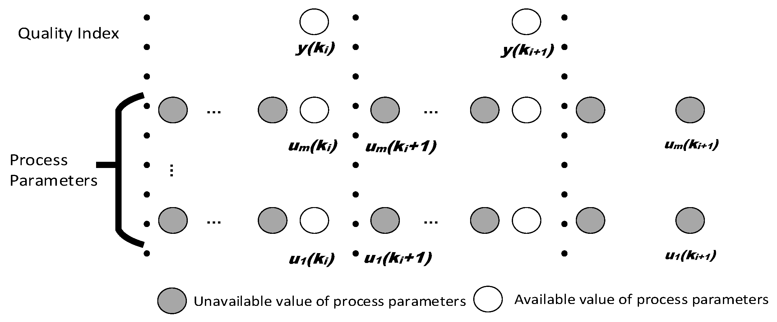
2. Problem Statement

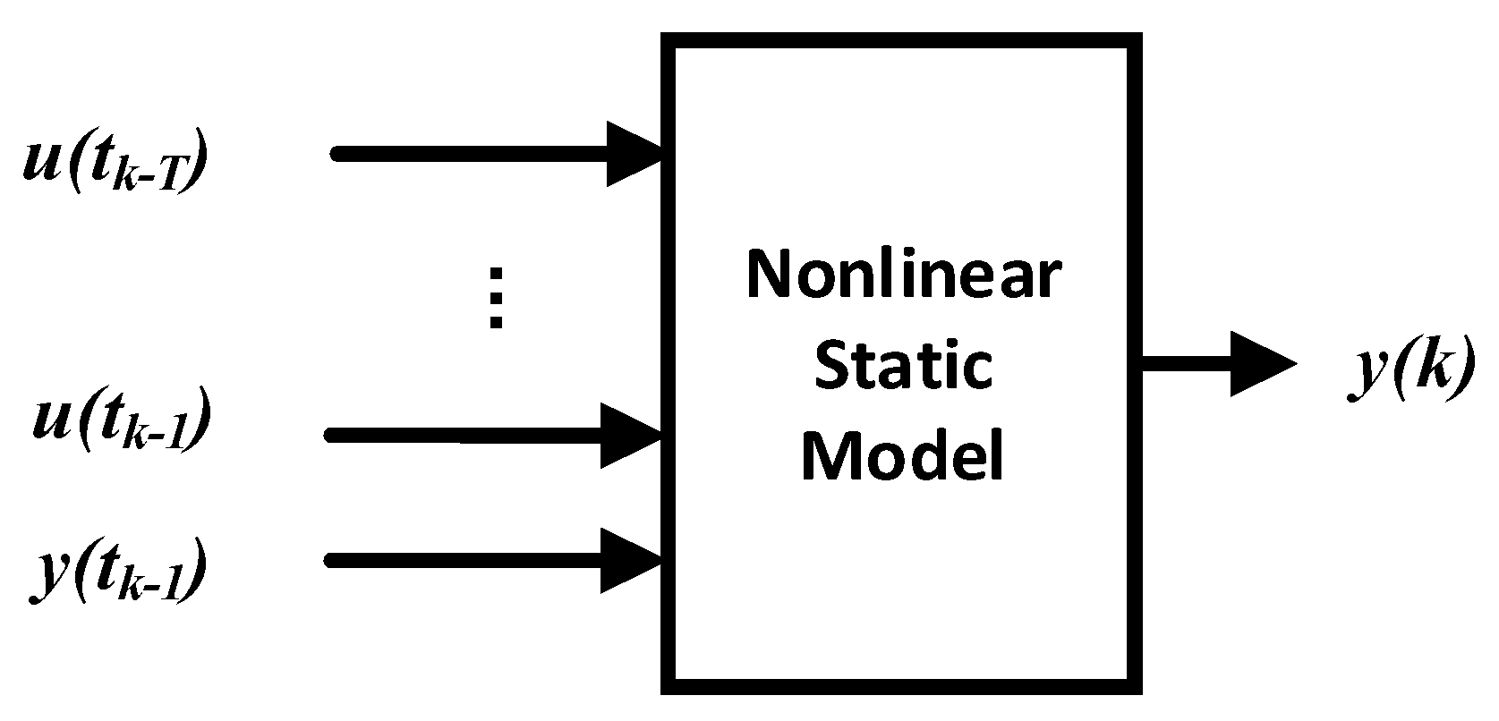
The chemical process is a sequential production. Generally, the continuous sampling of input variables can be obtained, with only the sparse sampling of the output variables being gained [25]. Only a small number of process parameters are used, while past data with a large amount of dynamic information are ignored [12], as shown in Figure 1.

The problem to be studied and solved in this paper is how to rationally integrate the dynamic characteristics of a chemical process into SSMI data, convert dynamic process data into static data, and establish an SSM and optimize the model parameters to achieve the purpose of the SSM prediction accuracy improvement.

3. DSSMI-AMWPDD

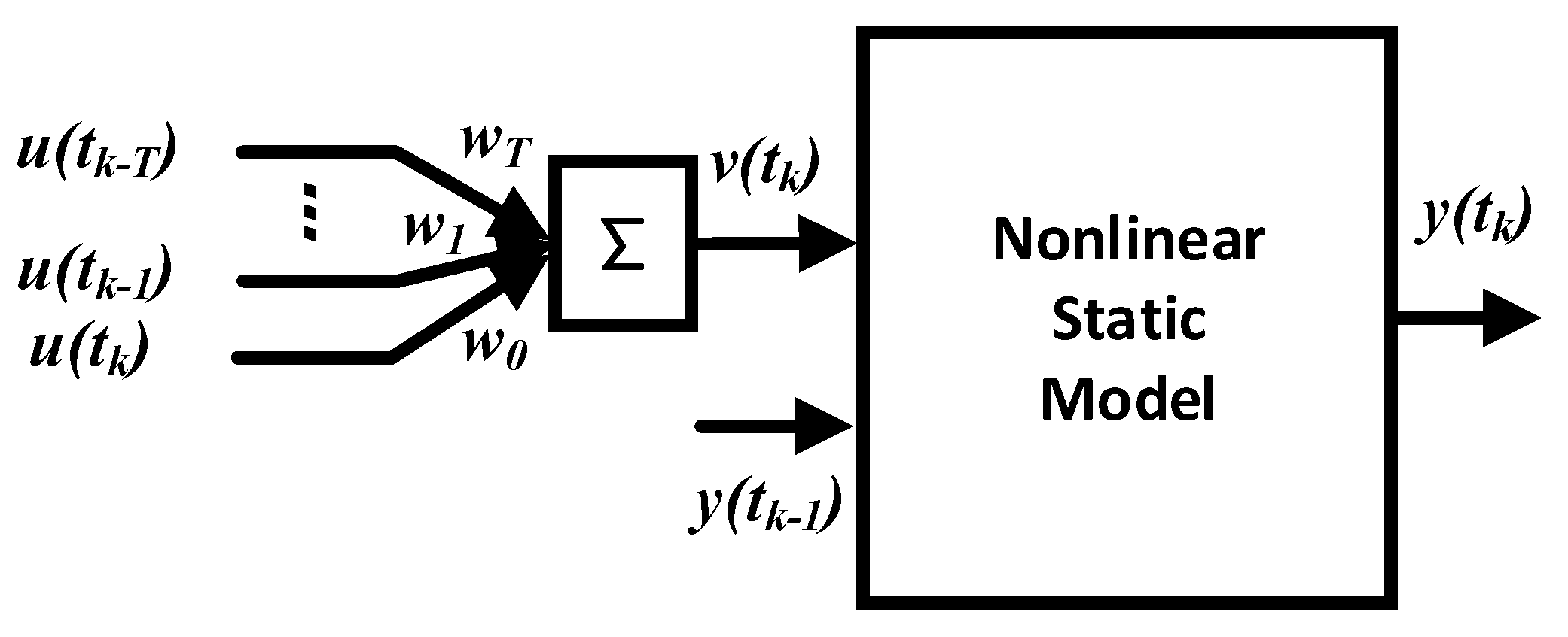
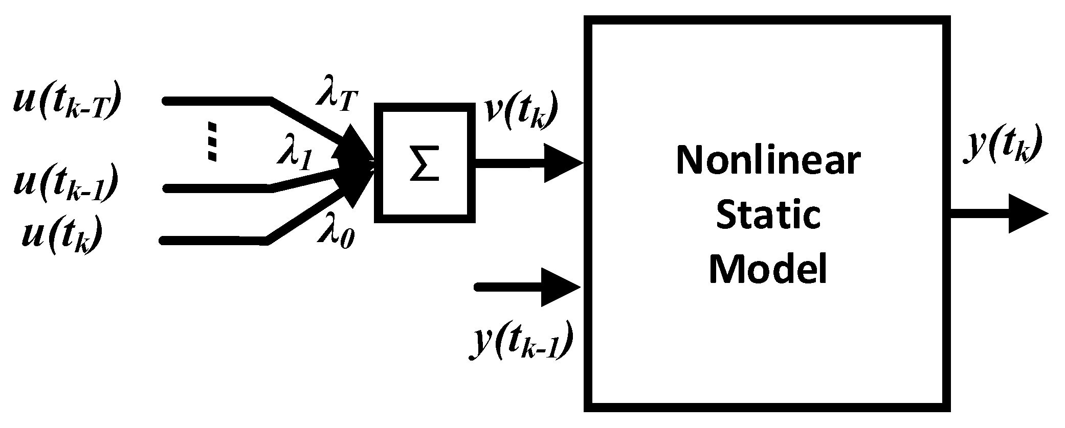
3.1. AMWPDD Sample Data Processing

Adding a large number of historical inputs not only increases the number and complexity of the parameters of the model but also causes the ill conditioning of the model due to the excessively high dimensionality of the input variables.

In consideration of the sustained influence of the auxiliary variable data on the dominant variables in the chemical process and the corresponding difficulty in determining the degree of such influence, and to reduce the number of input nodes and lower the complexity of the model, the ARMA model structure is used to establish the input data vector using historical inputs and historical outputs.

The conventional $ARMA\left(p, q\right)$ model is as follows [7]:

$$\{\begin{array}{c}{x}_t={\phi }_0+{\phi }_1{x}_{t-1}+\cdots +{\phi }_p{x}_{t-p}+{\epsilon }_t-{\theta }_1{\epsilon }_{t-1}-\cdots -{\theta }_q{\epsilon }_{t-q},{\phi }_p\ne 0,{\theta }_q\ne 0;\\ E\left({\epsilon }_t\right)=0,Var\left({\epsilon }_t\right)={\sigma }_{\epsilon }^2,E\left({\epsilon }_t{\epsilon }_s\right)=0,s\ne t\\ E\left(x_s{\epsilon }_t\right)=0,\forall s<t.\end{array}$$

(1)

in which p and q are the orders of the model, φ is the operator of the AR of order p, and θ is the operator of MA of order q.

The multipoint input ARMA model used in this paper is shown in Figure 2:

The generalized function of the multipoint input ARMA model shown in Figure 2 is expressed as:

$$y\left(k\right)=f\left(X\left(k\right),\theta \right)$$

(2)

$$X\left(k\right)=\left[u\left(t_{k-1}\right),\cdots ,u\left(t_{k-T}\right),y\left(t_k-1\right)\right]$$

(3)

Adding the output of the previous batch as an effective input into the modeled sample data can reduce the number of historical input nodes, reducing the number of model parameters and the complexity of the model [26], and lowering the possibility of morbidity in the model.

However, the multipoint input ARMA model shown in Figure 2 still has an incomplete model structure induced by numerous historical input nodes and the high model complexity.

To solve these problems, we combine the dynamic weighting model [27] with the ARMA model to realize the dynamic weighted fusion of the input nodes and hence reflect the dynamic characteristics of the process, as shown in Figure 3:

Its generalized function is expressed as:

$$y \left(t_k\right)=f\left(v\left(t_k\right),y\left(t_k-1\right),\theta \right)$$

(4)

$$v\left(t_k\right)={{\displaystyle \sum }}_{i=0}^T{w}_{i}u\left(t_{k-i}\right)$$

(5)

The dynamic weight directly reflects the dynamic characteristics of the process and affects the accuracy of the overall model. However, it is difficult to obtain accurate values of the dynamic weights. To solve this problem, this paper proposes an assumed condition suitable for most sequential chemical processes after a detailed site investigation of the chemical process.

If the value of the input node changes in different time periods, the further away an input point is from the output time, the less influence the value of the input node has on the change in the value of the output node.

The above assumption is explained as follows:

$$\Delta y\left(t_k\right)={{\displaystyle \sum }}_{\sigma =0}^T{\delta }_{\sigma }f\left(u_i\left(t_{k-\sigma }\right)\right),i=1,\cdots ,n$$

(6)

$${\delta }_{\sigma }=\{\begin{array}{c}\frac{1}{\left|t_k-t_{k-\sigma }\right|},\sigma \ne 0\\ 1,\sigma =0\end{array}$$

(7)

where ${\delta }_{\sigma }$ is the degree of influence in the input node value.

Based on the above assumptions, this paper introduces DF λ and uses the discount method [28,29] to dynamically discount-weigh the auxiliary variable values of different sampling time points in the same batch. By doing this, the impact of recent sample data on the model is enhanced, the role of past samples is reduced, the fusion of input node values from t_k to t_k+T is achieved, and the problem that the weight of the dynamic weighted model is difficult to judge is solved.

The structure of the AMWPDD proposed in this paper is shown in Figure 4:

Its generalized function is as follows:

$$y\left(t_k\right)=f\left(v\left(t_k\right),y\left(t_k-1\right),\theta \right)$$

(8)

$$v\left(t_k\right)={{\displaystyle \sum }}_{i=0}^T{\lambda }_{i}u\left(t_{k-i}\right)$$

(9)

where $v\left(t_k\right)$ is the process input data obtained by DF weighted fusion.

However, the transition time T of the input variable of the chemical process, that is, the HD length, is difficult to determine. To ensure the data integrity of the batch input and output variables, this paper proposes a calculation method of DF λ in combination with the above assumption.

DF λ numerical constraints:

(1)

λ₁ + λ₂ + …… + λ_T = 1;

(2)

λ₁ > λ₂ > …… > λ_T;

The calculation formula of DF λ is:

$${\lambda }_i={\eta }^i,i=0,1,2,\cdots ,T$$

(10)

$${\displaystyle \sum }_{i=1}^T{\eta }^i=1$$

(11)

One can obtain the dynamic value of DF λ_i, i = 1, 2, ⋯, T based on different transition times T by Equations (10) and (11), realize the dynamic calculation of the DF λ value, and obtain more accurate data fusion weights.

Then, the sample data set S for SSM modeling is:

$$S=\left\{\begin{array}{l}{v}_j\left(t_k\right),y\left(t_k-1\right)|k=1,2,\cdots ,M;j=1,2,\cdots ,N\\ y\left(t_k\right)|k=1,2,\cdots ,M\end{array}\right\}$$

(12)

where $v_j\left(t_k\right)$ is the j input variables at time $t_k, y\left(t_k\right)$ is the output variable at time $t_k, y\left(t_k-1\right)$ is the output variable at time t_k − 1, and $t_k\left(k=1,2,\cdots ,M\right)$ indicates the sampling time at which the system outputs M sample points.

On the basis of the sample data set S for the SSM, the SSM is established by the SSMI method.

3.2. LSSVM-Based SSMI

The least squares support vector machine (LSSVM) is a machine learning method proposed by Suykens [30] for solving the function estimation. It has better calculation speed, convergence precision and generalization performance and is more suitable for the small sample data SSMI of chemical processes [31].

The LSSVM model [32] is:

$$y\left(x\right)={\omega }^T\varphi \left(x\right)+b$$

(13)

where $\varphi (·)$ is a nonlinear transformation function, ω is an adjustable weight vector, and $b$ is an offset.

The objective function of LSSVM [33] is as follows:

$$minJ\left(\omega ,\xi \right)=\frac{1}{2}{\omega }^T\omega +\frac{C}{2}{{\displaystyle \sum }}_{i=1}^l{\xi }^T\xi$$

(14)

$$s.t.\hspace{1em}{y}_i={\omega }^T\phi \left(x_i\right)+b+{\xi }_i\left(i=1,2,\cdots ,l\right)$$

(15)

where $x_i\in R^n$ refers to the input vector, $y_i\in R$ represents the corresponding output vector, ${\xi }_i$ is the difference between the system output value and actual value, $C\ge 0$ represents a regularization parameter used to minimize the estimation error and control the function smoothness, $\phi (·)$ refers to a nonlinear mapping from the input space to the feature space, ω is the system weight, $b$ is an offset, and $s.t.$ indicates a constraint condition.

The Lagrange polynomial function of the optimization is solved by the Karush–Kuhn–Tucher (KKT) condition, and the LSSVM model for function estimation can be expressed as:

$$\widehat{y}=f\left(x\right)={{\displaystyle \sum }}_{i=1}^l\widehat{{\alpha }_i}K\left(x_i,x\right)+\widehat{b}$$

(16)

Since the radial basis kernel function is a kernel function that has been widely used [34], it is chosen in this paper:

$$k\left(x,x^{\prime }\right)=\exp \left\{-\frac{\Vert x-x^{\prime }{\Vert }^2}{2{\sigma }^2}\right\}, \sigma >0 is kernel radius$$

(17)

After the kernel function is determined, the error term penalizes the parameter C, and the kernel function parameter σ² affects the regression performance of the LSSVM method. However, they are difficult to determine. To ensure the optimal regression performance of the LSSVM, this paper uses PSO to optimize the error term penalty parameter C and the kernel function parameter σ².

4. Model Parameter Optimization Based on ωDPSO

To improve the prediction accuracy of SSM, the optimization objective is set to minimize the sum of the squared errors between the sample actual output data $y_0\left(t_k\right)$ and sample prediction output $y\left(t_k\right)$. The optimization objective function is as follows:

$$minJ=\frac{1}{M}{\displaystyle \sum }_{k=1}^M\Vert y\left(t_k\right)-y_0{\left(t_k\right)\Vert }^2$$

(18)

PSO [18] is an intelligent algorithm that simulates the predation behavior of birds and fish groups.

In PSO, each particle has independent position, velocity, and fitness for optimizing the target. PSO randomly sets a certain number of particles, initializes their positions and speeds, and completes the optimization process by iteration. The iterative process generally includes two optimal values: the Personal Best Value (pbest) and the Global Best Value (gbest); pbest represents the optimal fitness of the particle itself, and gbest refers to the optimal fitness of all particles. The particle updates its position and velocity by tracking two extreme values (pbest, gbest), and the updated formula is as follows:

$$v_{id}\left(t+1\right)=w\times v_{id}\left(t\right)+c_1\times rand()\times \left(p_{id}-x_{id}\left(t\right)\right)+c_2\times rand()\times \left(p_{gd}-x_{id}\left(t\right)\right)$$

(19)

$$x_{id}\left(t+1\right)=x_{id}\left(t\right)+v_{id}\left(t+1\right)$$

(20)

where v_id, x_id, and p_id represent the velocity, position, and personal best value, respectively, of particle i in iteration t; rand() is a random number between [0, 1]; c₁ and c₂ are learning factors, which represent the weights of the statistical acceleration terms that push each particle to the pbest and gbest locations; ω is the inertia weight; t is the number of iterations.

Since the inertia weight is related to the development and exploration ability of the particle, it affects the convergence of the algorithm [35,36]. A larger ω value is beneficial to jump out of a local optimum for global optimization; a smaller ω value is beneficial to local optimization and accelerates the convergence of the algorithm. When the search process follows a nonlinear and highly complex algorithm, the linearly decreasing inertia weight does not effectively reflect the actual search process [37]. At the same time, the inertia weight linear decreasing strategy based on the number of iterations has a weak partial search in the early iteration, and the particle might miss the optimal value even if it is close to the current value; in late iterations, the global search ability is weak, and it is easy to fall into the local optimum problem. In this paper, an ωDPSO is proposed, which improves the convergence of the algorithm by dynamically adjusting the inertia weight ω value, as shown in Figure 5:

The equation for the inertia weight is expressed as:

$$\omega =0.8-0.3\ast sawtooth\left(t,j/k\right)$$

(21)

As shown in Figure 5, compared with the inertia weight linear decreasing strategy based on the number of iterations, the inertia weight ω values proposed in this paper vary from large to small, then from small to large, and again from large to small, showing a periodic sawtooth fluctuation. As a result, the particles are periodically alternating between focusing on the global search and focusing on the local search. This balances the global search and the local search, avoids being trapped in a local optimum, improving the convergence of the PSO algorithm. At the same time, according to the ratio of the current iteration number to the total number of iterations, the ratio of the time prior to the peak within the cycle to the cycle time is adjusted so that the inertia weight ω increases rapidly and decreases slowly in early numerical iterations, grows and reduces slowly in the middle iterations, and rises slowly and decreases rapidly in the late iterations.

Through ωDPSO, the LSSVM SSMI method penalty parameter C and the kernel function parameter σ² are numerically optimized.

5. Simulation and Analysis

A CSTR is used as study objects to test the predictive performance of the SSMI method proposed in this paper for nonlinear dynamic time-varying chemical processes. The CSTR data comes from a computer simulation. In addition, to evaluate the performance of the proposed method, the dynamic and static data LSSVM SSM, PSO-LSSVM SSM, and ωDPSO-LSSVM soft sensor model of the CSTR object are established.

Given the commonality and universality of evaluation indices, including the mean absolute error (MAE), root mean square error (RMSE), and running time (RT), in regression analyses, this paper uses the RMSE in Equation (23) and the RT to evaluate the training performance of the SSM and the MAE in Equation (22) and the RMSE in Equation (23) to evaluate the prediction accuracy of the SSM:

$$MAE=\frac{1}{N}{\displaystyle \sum }_{i=1}^N\left|\widehat{y_i}-y_i\right|$$

(22)

$$RMSE=\sqrt{\frac{1}{N}{\displaystyle \sum }_{i=1}^N{\left|\widehat{y_i}-y_i\right|}^2}$$

(23)

where N is the total number of samples, $\widehat{y_i}$ is the predicted output value, and $y_i$ is the actual value.

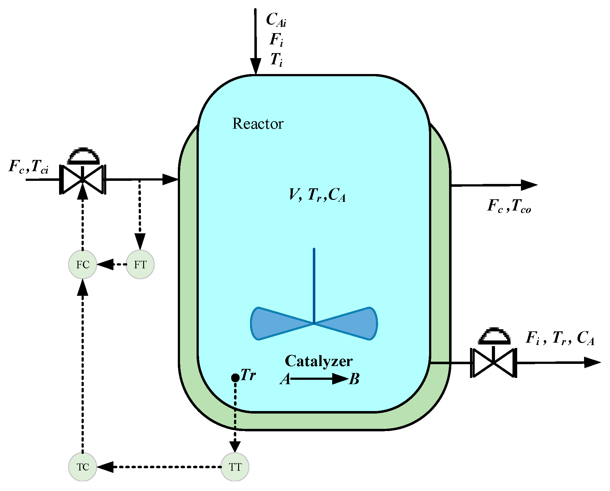
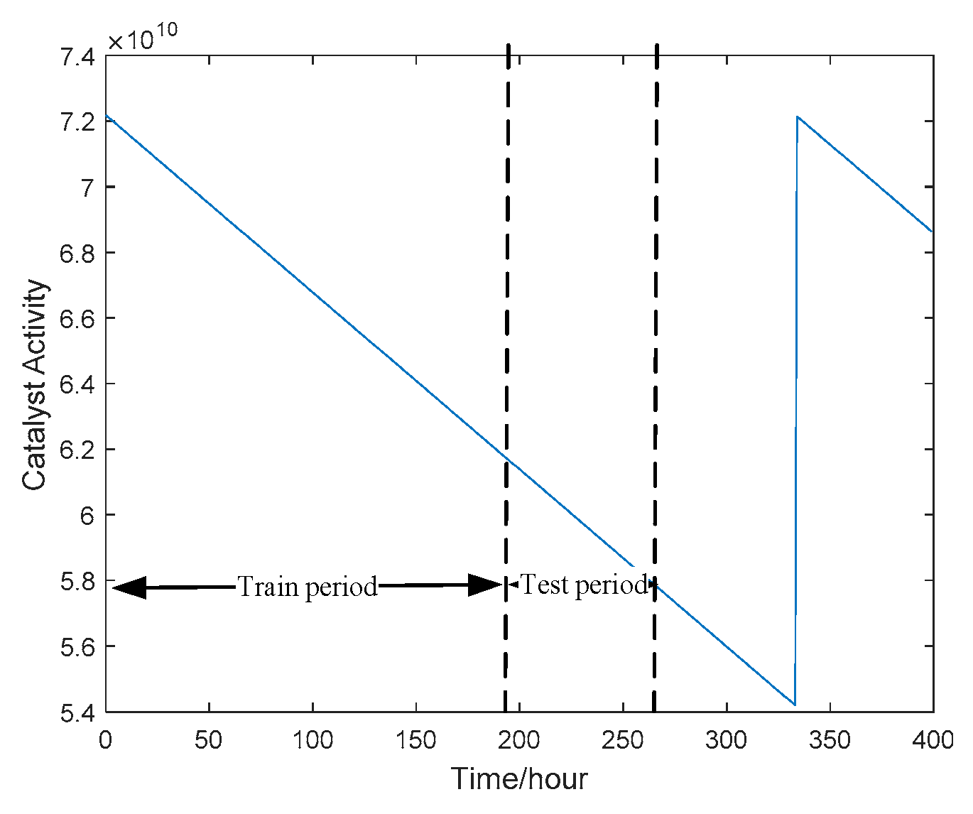
5.1. CSTR Simulation Experiment and Result Analysis

The continuous stirred tank reactor is the most important piece of equipment in many chemical and biochemical industries and has second-order nonlinear dynamic characteristics [38]. Therefore, it can be used to test the ability of the SSMI method to solve nonlinear and time-varying problems. The principle of the CSTR [39] is shown in Figure 6, with a description of each variable and the values of the steady-state operating points shown in

Table 1. Description and steady-state values of parameters of the CSTR.

Parameter	Description	Steady-State Value
Fi	Feed flow rate	100 L/min
CAi	Reactant concentration in the feed	1 mol/L
Ti	Feed temperature	350 K
V	Reactor volume	100 L
k0	Reaction speed	7.2 × 1010 min−1
Cp	Reactant specific heat capacity	1 cal/g/k
hA	Thermal conductivity	7 × 105 cal/min/K
Tci	Cooling water inlet temperature	350 K
Cpc	Cooling water specific heat capacity	1 cal/g/k

[40].

The concentration C_A of the raw material A in the reactor is considered to be the dominant variable of the SSM. The feed flow rate F_i, the cooling water flow rate F_c, and the reactor internal temperature T_r are treated as auxiliary variables of the SSM.

In the CSTR simulation process, the sampling periods of the auxiliary and dominant variables are set to 1 h and 12 h, respectively. The simulation time is set to 265 h, and a certain white Gaussian noise is added to each auxiliary variable. A total of 265 groups of usable data are obtained, 23 of which are labeled and the rest are dynamically unlabeled. The former 168 groups of data are used as the training sample set, and the latter 96 groups of data are used as the test sample set. A total of 22 groups of dynamic fusion data and static data with the same output are used as the SSMI samples. To simulate the reduction and recovery of the catalyst activity in the reactor, the catalyst activity k₀ is set for the data simulation based on the variation pattern in Figure 7, and the simulated data set is then normalized.

The following model structure based on static data modeling is used:

$${\widehat{y}}_s\left(t_k\right)=f_{sCSTR}\left(u_j\left(t_k\right)\right), j=1, 2, 3$$

(24)

With expert knowledge and the dynamic characteristics of the CSTR, the following model structure is adopted for dynamic fusion data-based modeling:

$${\widehat{y}}_d\left(t_k\right)=f_{dCSTR}\left(\begin{array}{l}{v}_j\left(t_k\right)\\ y\left(t_k-1\right)\end{array}\right), j=1, 2, 3$$

(25)

$$v_j\left(t_k\right)=f_{Dis}\left[\begin{array}{l}{u}_j\left(t_{k-11}\right)\\ ⋮ \\ u_j\left(t_{k-1}\right)\\ u_j\left(t_k\right)\end{array}\right]$$

(26)

where $y\left(t_k\right)$ represents the concentration in the reactor C_A at time t_k, $u_j\left(t_{k-T}\right)\left(1\le j\le 3,0\le T\le 11\right)$ represents the sampled value of the j^th auxiliary variable at time t_k-T, $v_j\left(t_k\right)$ is the discounted fusion value of $u_j\left(t_{k-T}\right)\left(1\le j\le 3,0\le T\le 11\right)$ and $\widehat{y}\left(t_k\right)$ represents the concentration in the reactor predicted by the SSM.

The parameters for the method comparison are set as follows:

LSSVM: $C=80, {\sigma }^2=20$

PSO-LSSVM: number of iterations: 100; number of particles: 20; $C\in \left[20,130\right] {\sigma }^2\in \left[20,130\right]$.

ωDPSO-LSSVM: number of iterations: 100; number of particles: 20; $C\in \left[20,130\right] {\sigma }^2\in \left[20,130\right]$.

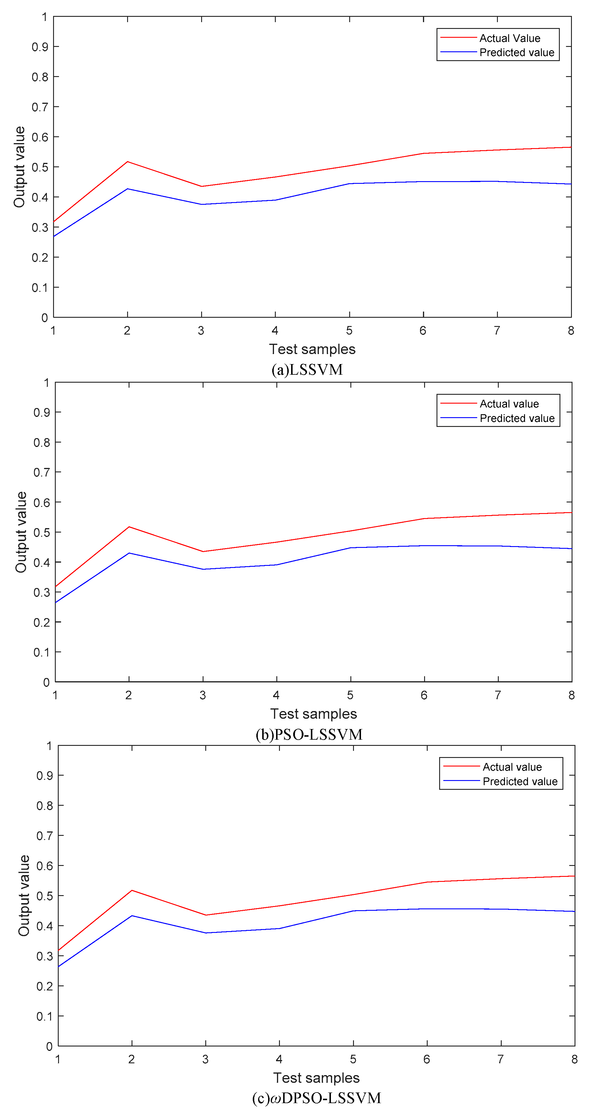
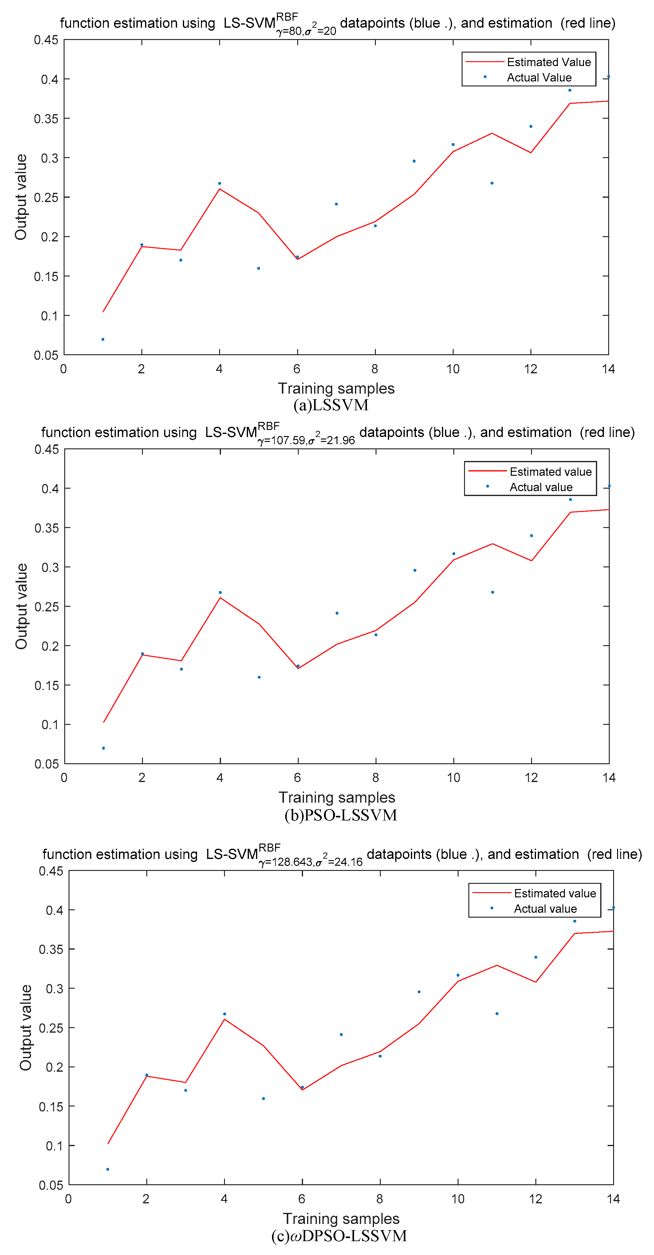
5.1.1. SSMI Based on Static Data

The SSMs of the above three methods are based on static data, wherein, for the PSO-LSSVM method, $C=101.79 \mathrm{and} {\sigma }^2=20.53$, and for the ωDPSO-LSSVM method, $118.13 \mathrm{and} {\sigma }^2=21.67$, as shown in Figure 8.

With white Gaussian noise added to the auxiliary variables, it can be seen from Figure 8a–c that the three SSMI methods all have large offsets. Combining the RMSE values of the model training performance shown in

Table 2. Comparison of CSTR performances of the different SSMs.

Soft Sensor	RMSE	Running Time(s)
LSSVM	0.0446	0.851
PSO-LSSVM	0.0440	26.520
ωDPSO -LSSVM	0.0439	22.744

, it can be seen that the models trained by PSO-LSSVM and ωDPSO-LSSVM are closer to the actual data. Compared with that of the LSSVM method, the RMSE index increases by 1.35% and 1.57%, respectively, and the RT index falls by factors of 30.16 and 25.73, respectively.

Compared to those of the PSO-LSSVM method, the RMSE and RT indices of the ωDPSO-LSSVM method rises by 0.23% and 14.24%, respectively.

The training performances of the different SSMI methods are shown in Table 2.

The performances of the different SSMI methods using test data set are compared, as shown in Figure 9.

It can be seen from Figure 9 that the prediction values by the LSSVM, PSO-LSSVM, and ωDPSO-LSSVM methods based on static data all show large offsets, and the prediction performance evaluation indices MAE and RMSE of each SSM are also poor. However, compared with those of the LSSVM method, the MAE values of the PSO-LSSVM and ωDPSO-LSSVM methods grow by 1.59% and 3.17%, respectively, and their RMSE values rise by 1.64% and 3.52%, respectively.

Compared to those of the PSO-LSSVM method, the MAE and RMSE values of the ωDPSO-LSSVM method increase by 1.6% and 1.9%, respectively, indicating a higher prediction accuracy.

The prediction performances of the different SSMI methods are shown in

Table 3. Comparison of CSTR performances of the different SSMs.

Soft Sensor	MAE	RMSE
LSSVM	0.0820	0.0853
PSO-LSSVM	0.0807	0.0839
ωDPSO -LSSVM	0.0794	0.0823

.

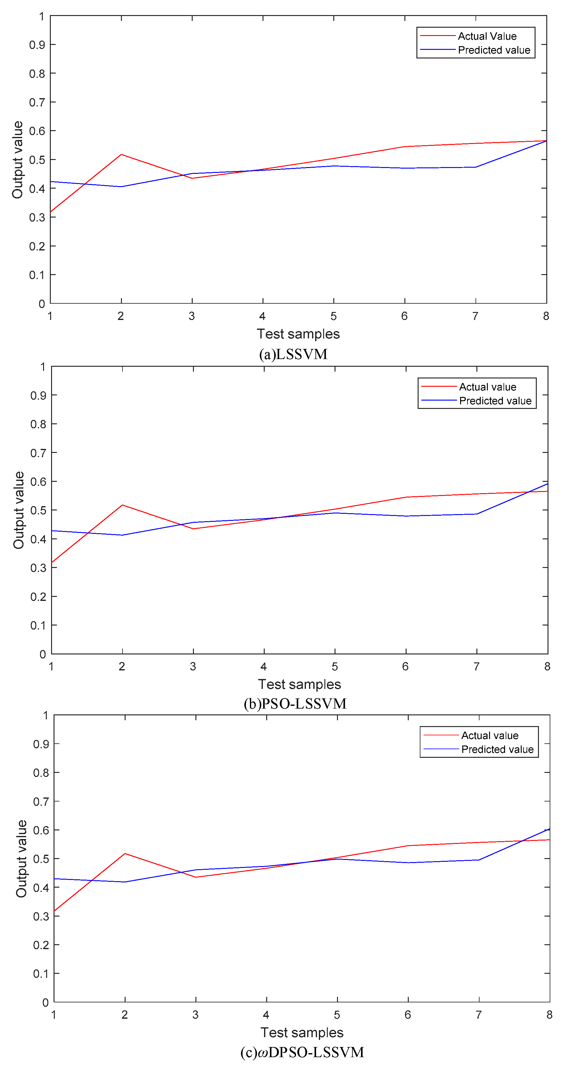
5.1.2. SSMI Based on Dynamic Fusion Data

The SSMs of the above three methods are established based on dynamic fusion data, wherein the PSO-LSSVM method, $C=107.59 \mathrm{and} {\sigma }^2=21.96$, and the ωDPSO-LSSVM method, $C=128.643 \mathrm{and} {\sigma }^2=24.16$, are shown in Figure 10.

As shown in Figure 10, the different SSMI methods have different training effects on the dynamic fusion data. Combined with the RMSE values of the models built by the different soft sensor methods, as listed in

Table 4. Comparison of CSTR performances of the different SSMs.

Soft Sensor	RMSE	Running Time(s)
LSSVM	0.0341	0.793
PSO-LSSVM	0.0328	28.94
ωDPSO -LSSVM	0.0327	22.143

, it found that, compared with those of the LSSVM method, the RMSE indices of the PSO-LSSVM and ωDPSO-LSSVM methods rise by 3.81% and 4.11%, respectively, and their RT indices decrease by factors of 35.49 and 26.92, respectively.

Compared with those of the PSO-LSSVM method, the RMSE and RT indices of the ωDPSO-LSSVM method reduce by 0.31% and 6.8%, respectively.

The training performances of the different SSMI methods are shown in Table 4:

The performances of the different SSMI methods using the test data set are compared, as shown in Figure 11.

A comparison of the prediction curves of the LSSVM, PSO-LSSVM, and ωDPSO-LSSVM methods in Figure 11 shows that the prediction curves of the PSO-LSSVM and ωDPSO-LSSVM methods are closer to the actual values. As seen in

Table 5. Comparison of CSTR performances of the different SSMs.

Soft Sensor	MAE	RMSE
LSSVM	0.0529	0.0683
PSO-LSSVM	0.0521	0.0650
ωDPSO -LSSVM	0.0511	0.0632

, compared with the those of the LSSM method, the MAE values of the PSO-LSSVM and ωDPSO-LSSVM methods grow by 1.51% and 3.4%, respectively, and their RMSE values rise by 4.83% and 7.47%, respectively. Compared with those of the PSO-LSSVM method, the MAE and RMSE values of the ωDPSO-LSSVM method increase by 1.92% and 2.77%, respectively.

The prediction performances of the different SSMI methods are shown in Table 5.

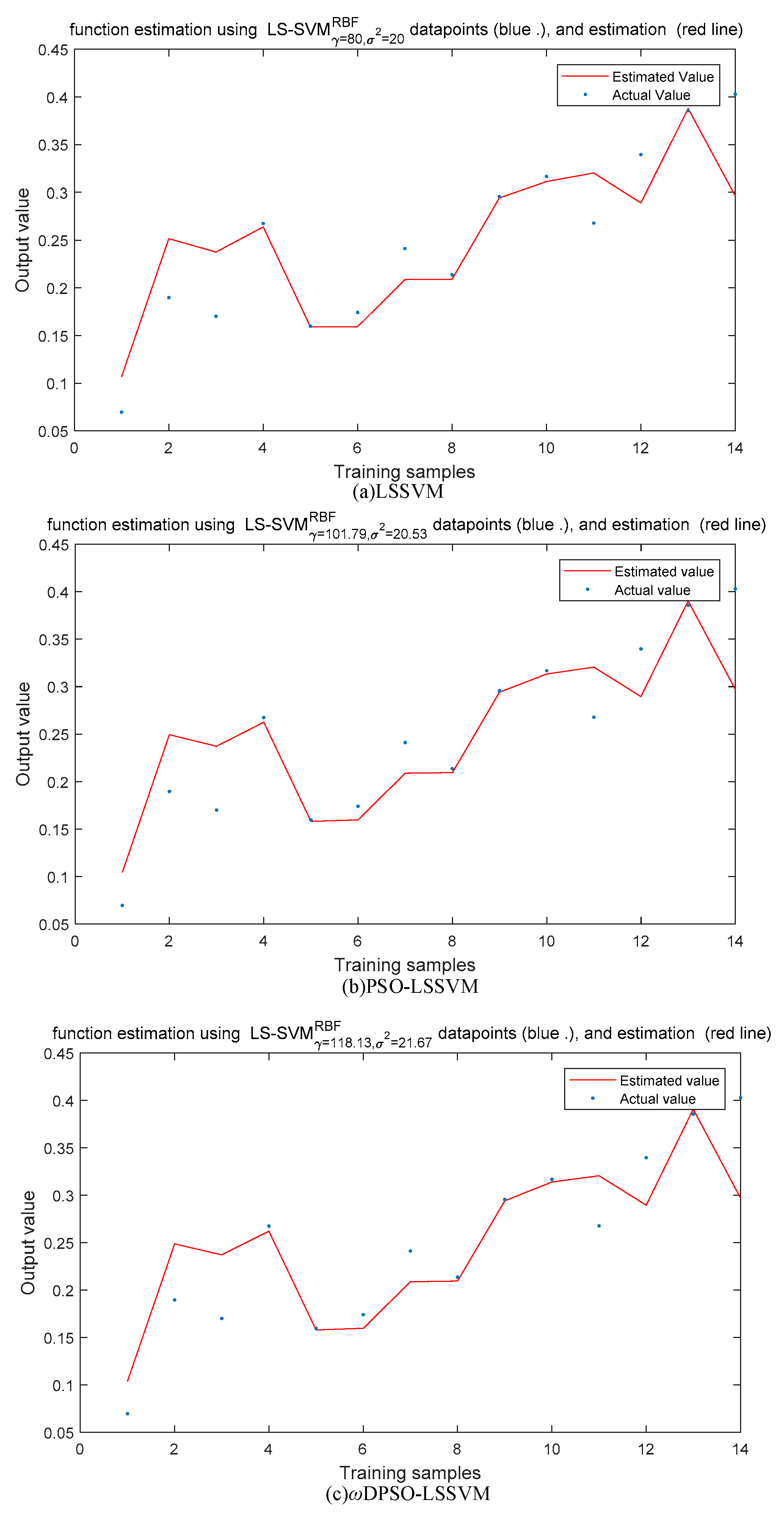
5.1.3. Comparison and Analysis

A comparison of Figure 8 and Figure 10, as well as Figure 9 and Figure 11, combined with the data analysis in Section 5.1.1 and Section 5.1.2, shows that, compared with that based on static data, the RMSE values of the model training results using the three methods based on dynamic fusion data rise by 23.54%, 25.46%, and 25.51%, respectively. Compared with those based on static data, the MAE values of the three methods based on dynamic fusion data grow by 35.49%, 35.44%, and 35.64%, respectively, and the RMSE values increase by 19.93%, 22.53%, and 23.21%, respectively. The models established via dynamic fusion data and the corresponding data prediction accuracy are better than those using static data. The main reason is that the chemical process is a continuous time series production process, and changes in the values of the auxiliary variables affect the values of the subsequent dominant variables. Modeling based only on the current static data is unable to reflect the process variation of the auxiliary variables, resulting in the poor training of the model and low precision of the data prediction. In view of the influence of the inertia weight coefficient ω on the convergence performance of the PSO method, the ωDPSO-LSSVM method achieves better prediction performance than the PSO-LSSVM method.

5.2. Simulation Experiment and Result Analysis

In Section 5.1, the simulation data of CSTR is used to experimentally verify the proposed DSSMI-AMWPDD method based on ωDPSO. A comparison of the modeling using dynamic fusion data and static data, as well as the experimental results of data prediction, proves that the SSM established by dynamic fusion data is superior to that those using static data in terms of the prediction model accuracy and data prediction precision. Additionally, this paper adopts the PSO-LSSVM method and the ωDPSO-LSSVM method to perform 10 trainings on CSTR data and selects the one with the best training effect as the experimental result, and the results show that the ωDPSO-LSSVM method achieves better prediction performance, shorter training time, and stronger convergence.

6. Conclusions

In this work, based on chemical processes as the research setting, the simulation modeling of CSTR simulation data shows that the AMWPDD proposed in this paper can reflect the dynamic changes of the chemical process and improve the accuracy of the SSM data prediction. Furthermore, the simulation results show that, compared with the standard PSO method, the ωDPSO method can better balance the local and global development capabilities, with faster convergence speed and higher convergence accuracy.

References

1. Wu, Y.; Luo, X. A novel calibration approach of soft sensor based on multirate data fusion technology. J. Process Control 2010, 20, 1252–1260. [Google Scholar] [CrossRef]
2. Gopakumar, V.; Tiwari, S.; Rahman, I. A deep learning based data driven soft sensor for bioprocesses. Biol. Eng. J. 2018, 136, 28–39. [Google Scholar] [CrossRef]
3. Kadlec, P.; Gabrys, B.; Strandt, S. Data-driven Soft Sensors in the process industry. Comput. Chem. Eng. 2009, 33, 795–814. [Google Scholar] [CrossRef]
4. Yan, W.; Guo, P.; Tian, Y.; Gao, J. A framework and modeling method of data-driven soft sensors based on semi-supervised gaussian regression. Ind. Eng. Chem. Res. 2016, 55, 7394–7401. [Google Scholar] [CrossRef]
5. Zhao, Y.; Fatehi, A.; Huang, B. A data-driven hybrid arx and markov-chain modeling approach to process identification with time varying time delays. IEEE Trans. Ind. Electr. 2017, 64, 4226–4236. [Google Scholar] [CrossRef]
6. Wang, X.; Huang, L.; Yang, C. Prediction model of slurry ph based on mechanism and error compensation for mineral flotation process. Chin. J. Chem. Eng. 2018, 26, 174–180. [Google Scholar] [CrossRef]
7. Liu, S.M.; Wu, Y.P.; Che, H.; Yipeng, W.; Han, C. Monitoring data quality control for a water distribution system using data self-recognition. J. Tsinghua Univ. (Sci. Technol.) 2017, 57, 999–1003. [Google Scholar] [CrossRef]
8. Di, K.S.; Wang, Y.H.; Shang, C.; Huang, D.X. Dynamic soft sensor modeling based on nonlinear slow feature analysis. Comput. Appl. Chem. 2016, 33, 1160–1164. [Google Scholar] [CrossRef]
9. Liu, J.; Vitelli, V.; Zio, E.; Seraoui, R. A novel dynamic-weighted probabilistic support vector regression-based ensemble for prognostics of time series data. IEEE Trans. Reliab. 2015, 64, 1203–1213. [Google Scholar] [CrossRef]
10. Osorio, D.; Ricardo Pérez-Correa, J.; Agosin, E.; Cabrera, M. Soft-sensor for on-line estimation of ethanol concentrations in wine stills. J. Food Eng. 2008, 87, 571–577. [Google Scholar] [CrossRef]
11. Shang, C.; Gao, X.; Yang, F.; Huang, D.X. Novel bayesian framework for dynamic soft sensor based on support vector machine with finite impulse response. IEEE Trans. Control Syst. Technol. 2014, 22, 1550–1557. [Google Scholar] [CrossRef]
12. Gao, X.; Yang, F.; Huang, D.; Ding, Y. An iterative two-level optimization method for the modeling of wiener structure nonlinear dynamic soft sensors. Ind. Eng. Chem. Res. 2014, 53, 1172–1178. [Google Scholar] [CrossRef]
13. Wang, Z.; Luo, X. Modeling study of nonlinear dynamic soft sensors and robust parameter identification using swarm intelligent optimization CS-NLJ. J. Process Control 2017, 58, 33–45. [Google Scholar] [CrossRef]
14. Yuan, P.; Zhang, B.; Mao, Z. A self-tuning control method for wiener nonlinear systems and its application to process control problems. Chin. J. Chem. Eng. 2017, 25, 193–201. [Google Scholar] [CrossRef]
15. Zhang, L.; Peng, X. Time series estimation of gas sensor baseline drift using arma and kalman based models. Sens. Rev. 2016, 36, 34–39. [Google Scholar] [CrossRef]
16. Sun, W.; He, Y.J.; Chang, H. Forecasting Fossil Fuel Energy Consumption for Power Generation Using QHSA-Based LSSVM Model. Energies 2015, 8, 939–959. [Google Scholar] [CrossRef]
17. Hong, X.; Chen, S. The system identification and control of hammerstein system using non-uniform rational b-spline neural network and particle swarm optimization. Neurocomputing 2012, 82, 216–223. [Google Scholar] [CrossRef]
18. Kennedy, J.; Eberhart, R.C. Particle Swarm Optimization. In Proceedings of the 1995 IEEE International Conference on Neural Networks, Perth, Australia, 27 November–1 December 1995; IEEE: Piscataway, NJ, USA, 1995; pp. 1942–1948. [Google Scholar]
19. Aburomman, A.A.; Reaz, M.B.I. A novel svm-knn-pso ensemble method for intrusion detection system. Appl. Soft Comput. 2015, 38, 360–372. [Google Scholar] [CrossRef]
20. Hu, W.; Yan, L.; Liu, K.; Wang, H. A short-term traffic flow forecasting method based on the hybrid PSO-SVR. Neur. Prof. Lett. 2016, 43, 155–172. [Google Scholar] [CrossRef]
21. Ma, D.; Tan, W.; Zhang, Z.; Hu, J. Gas emission source term estimation with 1-step nonlinear partial swarm optimization–Tikhonov regularization hybrid method. Chin. J. Chem. Eng. 2018, 26, 356–363. [Google Scholar] [CrossRef]
22. Wang, Y.; Hu, B.; Yang, X.; Wang, X.; Wang, J.; Huang, H. Prediction of flood season precipitation in southwest china based on improved pso-pls. J. Trop. Meteorol. 2018, 2, 163–175. [Google Scholar] [CrossRef]
23. Xiao, Y.; Kang, N.; Hong, Y.; Zhang, G. Misalignment Fault Diagnosis of DFWT Based on IEMD Energy Entropy and PSO-SVM. Entropy 2017, 19, 6. [Google Scholar] [CrossRef]
24. Guedria, N.B. Improved accelerated PSO algorithm for mechanical engineering optimization problems. Appl. Sofe Comput. 2016, 40, 455–467. [Google Scholar] [CrossRef]
25. Cao, P.; Luo, X. Modeling of soft sensor for chemical process. CIESC J. 2013, 64, 788–800. [Google Scholar] [CrossRef]
26. Zhang, D.; Cao, J.; Sun, L. Soft sensor modeling of moisture content in drying process based on LSSVM. Int. Conf. Electr. Meas. Instrum. 2009, 2, 989–993. [Google Scholar] [CrossRef]
27. Mejri, D.; Limam, M.; Weihs, C. A new dynamic weighted majority control chart for data streams. Soft Comput. 2016, 22, 511–522. [Google Scholar] [CrossRef]
28. Brekelmans, R.; Hertog, D.D.; Roos, K.; Eijgenraam, C. Safe dike heights at minimal costs: The nonhomogeneous case. Oper. Res. 2012, 60, 1342–1355. [Google Scholar] [CrossRef]
29. Triantafyllopoulos, K. Multivariate discount weighted regression and local level models. Comput. Stat. Data Anal. 2006, 50, 3702–3720. [Google Scholar] [CrossRef]
30. Suykens, J.; Johan, A.K. Least squares support vector machines. Int. J. Circ. Theor. Appl. 2002, 27, 605–615. [Google Scholar] [CrossRef]
31. Zhao, X.; Gao, Q.; Tang, C.; Liu, X.; Song, J.; Zhou, C. Prediction of reservoir parameters of delta lithologic reservoirs based on support vector regression and well-steering. Oil Geophys. Prospect. 2016, 51. [Google Scholar] [CrossRef]
32. Li, C.X.; Ding, X.D.; Zheng, X.F. Predicting non-Gaussian wind velocity using hybridizing intelligent optimization based LSSVM. J. Vib. Shock 2017, 36, 52–58. [Google Scholar] [CrossRef]
33. Suykens, J.A.K.; Brabanter, J.D.; Lukas, L.; Vandewalle, J. Weighted least squares support vector machines: Robustness and sparse approximation. Neurocomputing 2002, 48, 85–105. [Google Scholar] [CrossRef]
34. Roushangar, K.; Saghebian, S.M.; Mouaze, D. Predicting characteristics of dune bedforms using PSO-LSSVM. Int. J. Sediment Res. 2017, 32, 515–526. [Google Scholar] [CrossRef]
35. Jiang, C.; Zhao, S.; Shen, S.; Guo, L. Particle swarm optimization algorithm with sinusoidal changing inertia weight. Comput. Eng. Appl. 2012, 48, 40–42. [Google Scholar] [CrossRef]
36. Zhu, L.X.; Ling, J.; Wang, B.; Hao, J.; Ding, Y. Soft-sensing modeling of marine protease fermentation process based on improved PSO-RBFNN. CIESC J. 2018, 69, 1221–1227. [Google Scholar] [CrossRef]
37. Xu, B.; Wang, Y.; Wang, F.; He, M.; Wang, M.; Xie, Y. Prediction of package volume based on improved PSO-BP. Comput. Integr. Manuf. Syst. 2018, 24, 1871–1879. [Google Scholar] [CrossRef]
38. Sinha, A.; Mishra, R. Control of a nonlinear continuous stirred tank reactor via event triggered sliding modes. Chem. Eng. Sci. 2018, 187, 52–59. [Google Scholar] [CrossRef] [Green Version]
39. Shao, W. Adaptive Soft Sensor Modeling Based on Local Learning; China U Petrol: Qingdao, China, 2016. [Google Scholar]
40. Khatibisepehr, S.; Huang, B.; Xu, F.; Espejo, A. A bayesian approach to design of adaptive multi-model inferential sensors with application in oil sand industry. J. Process Control 2012, 22, 1913–1929. [Google Scholar] [CrossRef]
Figure 1. Irregular quality sample in the chemical process.
Symmetry 11 01414 g001
Figure 2. Multipoint input ARMA model structure.
Symmetry 11 01414 g002
Figure 3. Dynamic weighted ARMA model structure.
Symmetry 11 01414 g003
Figure 4. Discount-weighted ARMA model structure.
Symmetry 11 01414 g004
Figure 5. Dynamic adjustment of inertia weight ω in 100 iterations.
Symmetry 11 01414 g005
Figure 6. The principle of the CSTR.
Symmetry 11 01414 g006
Figure 7. Variation pattern of catalyst activity k0.
Symmetry 11 01414 g007
Figure 8. Modeling data training for the different SSMI methods. (a) The training curve based on LSSVM; (b) The training curve based on PSO-LSSVM; (c) The training curve based on ωDPSO-LSSVM.
Symmetry 11 01414 g008
Figure 9. Prediction of test data by the different SSMI methods. (a) The prediction curve based on LSSVM; (b) The prediction curve based on PSO-LSSVM; (c) The prediction curve based on ωDPSO-LSSVM.
Symmetry 11 01414 g009
Figure 10. Modeling data training for the different SSMI methods. (a) The training curve based on LSSVM; (b) The training curve based on PSO-LSSVM; (c) The training curve based on ωDPSO-LSSVM.
Symmetry 11 01414 g010
Figure 11. Prediction of test data by the different SSMI methods. (a) The prediction curve based on LSSVM; (b) The prediction curve based on PSO-LSSVM; (c) The prediction curve based on ωDPSO-LSSVM.
Symmetry 11 01414 g011