Article

Large-Eddy Simulation of an Asymmetric Plane Diffuser: Comparison of Different Subgrid Scale Models

1
College of Automotive Engineering, Jilin University, Renmin Street No. 5988, Changchun 130012, China
2
State Key Laboratory of Automotive Simulation and Control, Jilin University, Renmin Street No. 5988, Changchun 130012, China
3
Department of Mechanical Engineering, Osaka University, 2-1 Yamada-oka, Suita-city, Osaka 565-0871, Japan
*
Author to whom correspondence should be addressed.
Symmetry 2019, 11(11), 1337; https://doi.org/10.3390/sym11111337
Submission received: 14 September 2019 / Revised: 20 October 2019 / Accepted: 21 October 2019 / Published: 29 October 2019
(This article belongs to the Special Issue Aero/Hydrodynamics and Symmetry)

Abstract

:
Large-eddy simulation (LES) of separated turbulent flow through an asymmetric plane diffuser is investigated. The outcome of an actual LES depends on the quality of the subgrid-scale (SGS) model, as well as the accuracy of the numerical method used to solve the equations for the resolved scales. In this paper, we focus on the influence of SGS models for LES of the diffuser flow through using a high-order finite difference method to solve the equations for the resolved scales. Six resolutions are computed to investigate the influence of mesh resolution. Four existing SGS models, a new one-equation dynamic SGS model and a direct numerical simulation (DNS) are conducted in the diffuser flow. A series of computational analyses is performed to assess the performance of different SGS models on the coarse grids. By comparison with the experiment and DNS, the results produced by the new one-equation dynamic model give better agreement with experiment and DNS than the four other existing SGS models.

1. Introduction

Diffusers are ubiquitous in engineering applications. Usually simple in design, they serve to increase the static pressure of a flow by reducing its velocity, albeit often with significant losses. It has a simple design, but it develops complex three-dimensional flow features. A stable separation bubble forms early in the expanding section of the diffuser and spreads across one of the two expanding walls of the diffuser. The flow eventually reattaches in a straight exhaust duct where further pressure recovery occurs. Because of its simple three-dimensional geometry and the existence of a high quality velocity dataset, this diffuser has become a popular test case for measurement of mild separation and validating numerical simulations. However, accurate measurement and prediction of the pressure-driven separation in diffusers has always been challenging in fluid mechanics. In an experimental setup of the diffuser, the first challenge is achieving spanwise homogeneity of turbulence due to the presence of sidewalls producing strong backflow. The point of separation and the extent of the flow reversal zone in diffusers are particularly sensitive to the inlet condition [1]. In a numerical simulation of the diffuser, the presence of an adverse pressure gradient and the formation of an unsteady separation bubble make this flow very sensitive and difficult to predict with numerical means.
Two canonical laboratory incompressible diffuser flows have emerged as standard test-flows in the past: the diffuser studied by Azad [2] and the diffuser studied by Obi et al. [3]. The diffuser studied by Obi et al. [3] is selected in this paper since it has several desirable features. Firstly, the fully developed channel flow is utilized as the inlet condition. Flow in a duct with smooth parallel walls was fully investigated by Kim et al. [4]. For validating the simulation of a separating flow in diffusers. it is vitally significant to know accurately the statistics of the upstream flow because the separation bubble is so sensitive to upstream conditions. Secondly, the flow in this diffuser has rich flow physics, such as pressure-driven separation from a smooth wall, subsequent reattachment, and redevelopment of the downstream boundary layer, which are challenges for large eddy simulation (LES) with subgrid scale mode (SGS) models. Thirdly, based on the mean center velocity U c and the inlet duct of height H, the Reynolds number of the inlet channel flow is 7488. The corresponding Reynolds number based on the friction velocity is 407. A direct numerical simulation (DNS) of a diffuser flow is feasible at this Reynolds number, thus the DNS data can be used as supplementary benchmarks for assessing different SGS models [5]. Moreover, this Reynolds number is high enough that the flow is not sensitive to this parameter [6].
Actually, the diffuser studied by Obi et al. has been applied as a test flow in Reynolds-averaged Navier–Stokes (RANS) simulations, LES studies and DNS. Obi et al. [3] demonstrated that the standard k ϵ model fails to accurately predict the separation bubble in the diffuser. Durbin [7] proposed the k ϵ ν 2 model for separated flow and validated his new model in asymmetric plane diffuser with satisfactory accuracy in comparison with measurement. Iaccarino [8] investigated the turbulent flow in an asymmetrical two-dimensional diffuser using three commercial CFD codes: CFX, Fluent, and star-CD. El Behery and Hamed [9] presented a comparative study of turbulence models performance for the separating flow in a planar asymmetric diffuser, in which the steady RANS equations for turbulent incompressible fluid flow and six turbulence closures are used. Schneider et al. [10] performed the LES and RANS calculations for two asymmetrical three-dimensional diffusers and validated LES with wall function delivering the results within the accuracy of experimental data. Abe and Ohtsuka [11] investigated high Reynolds-number complex turbulent flows in a 3D diffuser using LES and hybrid LES/RANS models. Kaltenbach et al. [6] elaborately studied the flow in a planar asymmetric diffuser using LES with the dynamic Smagorinsky model. The overall good agreement of simulation results and measurement is obtained and it is found that the SGS model plays a significant role for both mean momentum and turbulent kinetic energy balances. Schluter et al. [12] compared LESs with no subgrid model, the standard Smagorinsky model, the dynamic Smagorinsky model and the dynamic localization model in a separated plane diffuser and demonstrated the dynamic localization model performing the best agreement with measurement. Kobayashi et al. [13] tested their own coherent structures model through some complex geometries in which the asymmetric plane diffuser is included. Taghinia et al. [14] developed a one-equation subgrid scale model with a variable eddy-viscosity coefficient for LES and validated the model in complex separated and reattaching turbulent flows, i.e., the turbulent flow through an asymmetric planar diffuser. Shuai and Agarwal [15] proposed a new one-equation eddy-viscosity model from the two-equation k-kL model. The new turbulence model is used to simulate an asymmetric plane diffuser and improved the accuracy of the flow simulations compared to the one-equation Spalart–Allmaras model. DNS of turbulent flow through an asymmetric plane diffuser was performed by Ohta and Kajishima [5] using a high-order finite difference method. The DNS results from this type of field can be used as one of the benchmarks for numerical simulation schemes and SGS models.
With increasing computing power, LES is more widely used in three-dimensional, unsteady complex flows. In LES technique, turbulent motions are separated into large-scale and small-scale contributions by using a filtering operation in which the large-scale fluid motions are directly calculated, whereas the unresolved SGS motions are modeled. The outcome of an actual LES therefore depends on the quality of the SGS model, as well as the accuracy of the numerical method used to solve the equations for the resolved scales. The important interactions between the resolved large eddies and unresolved SGS eddies, in the case of fully developed isotropic homogeneous turbulent flows, can be reduced to be seen as that of the energy transfers by omitting a portion of information included in the SGS eddies, for instance, the structural information associated to the anisotropy. It has been shown [16] that the energy transfer between SGS eddies and large eddies mainly exhibit two mechanisms: a forward energy transfer from large eddies to the SGS eddies and a backward transfer to the resolved scales, which, it seems, is much weaker in intensity. The SGS models are responsible for describing the desired dissipation or energy production effects.
In the present study, we focus on the influence of SGS models for LES of the separated turbulent flow in an asymmetric diffuser on the relative coarse mesh through using a high-order finite difference method to solve the equations for the resolved scales. Four existing SGS models, namely the Smagorinsky model [17], the dynamic Smagorinsky model [18,19], the one-equation model [20] and the one-equation dynamic model [21], and a new dynamic one-equation SGS model are investigated in diffuser flow. The Smagorinsky model, which can give a moderately accurate magnitude of energy transfer, is a simple and robust eddy viscosity model; however, it uses a priori model parameter. In the dynamic Smagorinsky model, the model coefficient is dynamically decided from the resolved scales to the unresolved SGS ranges based on an assumption of the scale invariance. However, the clipping procedure or averaging operation is still required in a homogeneous direction or in the global volume of domain. The one-equation model directly uses the information concerned with the SGS motions, i.e., the SGS kinetic energy, to decide the eddy viscosity, in which a transport equation of the SGS kinetic energy is solved and local equilibrium hypothesis of previous models can be removed. The one-equation dynamic model is a modification of the standard one-equation model, in which the production of SGS kinetic energy and the energy loss in large-scale portion are treated with different dynamic mechanisms, i.e., the production term in SGS kinetic energy transport equation is solved using a SGS model based on the resolved scales such as the dynamic Smagorinsky model, while the eddy viscosity in the filtered equation of motion is determined from information of unresolved scales—the transport equation of SGS kinetic energy. Since the test filtering operation is required in the one-equation dynamic model, all undesirable features and inconsistencies related to the test filtering operation are retained. The computation cost of solving an additional transport equation, as well as a dynamic procedure over test filter in the one-equation dynamic model is relatively huge. Thus, these properties still limit its application for the simulation of turbulent flows in complex geometries. It is necessary to continue the search for a new one-equation dynamic model that performs as well as the one-equation dynamic model, while the new model does not require any test filter and is not more expensive in terms of computational cost than the standard one-equation model.
Therefore, the goal of this study is to develop a new one-equation dynamic SGS model and examine the performance of the new SGS model and four existing SGS models on the flow prediction of pressure-driven separation in a diffuser by using a high-order finite difference method to solve the equations for the resolved scales. In addition, we examine the choice of mesh resolution of an asymmetric plane diffuser.

2. SGS Models

Applying a filter with scale Δ , and assuming the filtering operations are commuting with the operations of differentiation, the filtered Navier–Stokes (N-S) equation for LES of incompressible flows can be given as:
u ¯ i t + u ¯ i u ¯ j x j = 1 ρ p ¯ x i + ν 2 u ¯ i x j x j τ i j x j , u ¯ i x i = 0 .
where the SGS stress tensor is defined as τ i j = u i u j ¯ u ¯ i u ¯ j . A index notation is utilized to represent the components, in which the coordinates x 1 , x 2 and x 3 are denoted as streamwise, wall-normal and spanwise directions, respectively, and the corresponding velocity components are presented as u, v and w. Throughout this paper, summation convention is implied for repeated index.
As Boussinesq proposed, the SGS stress can be modeled as:
τ i j a x i x i τ i j 1 3 τ k k δ i j = x i 2 ν s g s S ¯ i j ,
in which τ i j a is the anisotropic component of τ i j ; S ¯ i j is the characteristic filtered rate-of-strain tensor and is defined as ( u ¯ i / x j + u ¯ j / x i ) / 2 ; and the coefficient of proportionality ν s g s is the SGS viscosity that remains to be evaluated by a SGS model.

2.1. Smagorinsky Model (SM)

Using the local equilibrium assumption, i.e., the dissipation rate of SGS energy is in balance with the production rate, the Smagorinsky model can be obtained for LES:
ν s g s = ( C s Δ ) 2 | S ¯ | ,
in which C s is a constant and taken to be 0.1 in this study. | S ¯ | denotes the norm of the rate-of-strain tensor and is defined as 2 S ¯ i j S ¯ i j . For wall-resolved LES, to make sure that modeled SGS stresses exhibit the near-wall behavior, a damping function f s has to be incorporated with the Smagorinsky model:
ν s g s = ( C s f s Δ ) 2 | S ¯ | .
The van Driest function is employed as the damping function:
f s = 1 e x p y + A + ,
in which the non-dimensional constant A + 25 and y + = y u τ / ν . For the separated flow in an asymmetric diffuser, it would be challenging to determine the friction velocity u τ in the vicinity of a separation point due to u τ = 0 . This is why few researchers try to use the Smagorinsky model for LES to simulate the diffuser flow. Even though the Smagorinsky model is applied in diffuser, its results are far from satisfactory. For example, Schluter et al. [12] found the flow separation was predicted on the upper wall instead on the inclined wall using the Smagorinsky model. In this study, an interesting method that u τ is determined by a linear interpolation is used in Smagorinsky model.
The two-dimensional schematic of Obi et al. diffuser is shown in Figure 1, in which the expansion ratio and expansion part of the diffuser is 4.7 and 21 H , respectively. A Cartesian coordinate system with the origin on the upper wall where the inlet channel wall and the deflected wall form a corner is used to define x in the streamwise direction and y in the downward wall-normal direction. Then, y + in diffuser can be approximately defined as (see Appendix A):
y + ( x , y ) = R e τ 0 · min ( y , 1 y ) / H , x 0 R e τ 0 · ( 1 3.7 / 4.7 · x / H ) · min [ y , Y ( x ) y ] / H , 0 < x 21 H R e τ 0 / 4.7 · min ( y , 4.7 H y ) / H , x > 21 H .
Here, R e τ 0 denotes the Reynolds number based on the friction velocity found in the inlet of duct. Y ( x ) means the local width of expansion in diffuser.

2.2. Standard Dynamic Smagorinsky Model (DSM)

Applying the test filter on the grid-filtered N-S equations, the Germano identity can be defined as
L i j = T i j τ ˜ i j = u ¯ i u ¯ j ˜ u ¯ ˜ i u ¯ ˜ j ,
where L i j can be calculated based on the resolved scales, T i j = u i u j ¯ ˜ u ¯ i ˜ u ¯ j ˜ represents the residual turbulent stress at a test-filter scale Δ ˜ , and can be given as
T i j 1 3 δ i j T k k = 2 C Δ ˜ 2 | S ¯ ˜ | S ¯ ˜ i j .
On substituting Equations (2) and (8) into Equation (7) and assuming Δ ¯ and C are constant inside the test filter, an equation for determining C is obtained:
L i j 1 3 δ i j L k k = 2 C Δ ¯ 2 M i j ,
where
M i j = Δ ˜ 2 Δ ¯ 2 | S ¯ ˜ | S ¯ ˜ i j | S ¯ | S ¯ i j ˜ .
Minimization of the error of Equation (9) over all independent tensor components [19], as well as over some averaging region of statistical homogeneity, leads to
C = 1 2 Δ ¯ 2 L i j M i j M i j M i j .

2.3. Standard One-Equation Model (OM)

The SGS eddy viscosity ν s g s is represented as ν s g s = C ν Δ ¯ ν k s g s by the dimensional analysis, where k s g s = ( u i u i ¯ u ¯ i u ¯ i ) / 2 = τ i i / 2 , i.e., the SGS kinetic energy. k s g s is evaluated by solving an evolution equation
k s g s t + u ¯ j k s g s x j = τ i j S ¯ i j C ε k s g s 3 / 2 Δ ε w + x j C d Δ ν k s g s + ν k s g s x j ,
which was theoretically derived by the authors of [22,23,24]. For meeting the correct asymptotic behavior to the wall, an additional modification was proposed by Okamoto & Shima [24] for the characteristic length Δ ν and additional dissipation term ε w , i.e.,
Δ ν = Δ ¯ 1 + C k Δ ¯ 2 S ¯ 2 / k s g s ,
ε w = 2 ν k s g s x j k s g s x j .
Non-dimensional constants associated with one-equation model are as follow: C ν = 0.05 , C ε = 0.835 , C d = 0.10 , and C k = 0.08 .

2.4. One-Equation Dynamic Model (ODM)

Kajishima and Nomachi [21] considered that the dynamic procedure (that is, Section 2.2 ) is suitable for the determination of energy transfer from resolved scales to SGS components since this transfer is regarded to be local and instantaneous, whereas the energy loss in large-scale portion is considered from the historic effect of SGS turbulence due to the transport. Thus, the dynamic procedure is applied to the production term in the transport equation of k s g s , while the SGS eddy viscosity in the filtered N-S equation is determined by using k s g s of Equation (12). The first term in the right-hand side of Equation (12) is given by
τ i j S ¯ i j = C s Δ ¯ 2 | S ¯ | 3 ,
where C s is calculated by the dynamic procedure of Equation (11). It should be noted that C s in the ODM model does not require any averaging over homogeneous direction or ad hoc clipping technique to avoid negative Smagorinsky constants. The negative value for C s is acceptable and it results in the decrease in k s g s . However, the computation of the test filter to evaluate the Germano Identity L i j and the parameter M i j is still required.

2.5. One-Equation Vreman Model (OVM)

Since the test filtering operation is required in the ODM model, all undesirable features and inconsistencies related to the test filtering operation are retained. The computation cost of solving an additional transport equation, as well as a dynamic procedure over test filter in the ODM model is relatively huge. Thus, these properties still limit its application for the simulation of turbulent flows in complex geometries. It is necessary to continue the search for a new one-equation dynamic model that performs as well as the ODM model, while not requiring any test filter and not being more expensive in terms of computational cost than the standard one-equation model.
Vreman [25] proposed a SGS model for the LES of turbulent shear flows (henceforth, referred to as Vreman model). Vreman model is essentially not more complicated than the Smagorinsky model, but is able to adequately handle turbulent as well as transitional flow. The model is expressed in first-order derivative, and does not involve test filtering, averaging, or clipping procedures. From two test cases of a transitional and turbulent mixing layer at high Reynolds number and a turbulent channel flow, Vreman model is found to be more accurate than Smagorinsky model and as good as the standard dynamic Smagorinsky model. Because of these desirable properties, it seems to be particularly pertinent for incorporating Vreman model into the ODM model to develop a new one-equation dynamic model that is suitable for LES of turbulent flows in complex geometries. In the new model, the production term in the transport equation of k s g s (Equation (12)) is represented as:
τ i j S ¯ i j = C v m + B β α i j α i j | S ¯ | 2 ,
where
B β = β 11 β 22 β 12 2 + β 11 β 33 β 13 2 + β 22 β 33 β 23 2 ,
β i j = Δ m 2 α m i α m j , α i j = u ¯ j x i ,
C v m + = C v m | Ω ¯ | / | S ¯ | , | Ω ¯ | / | S ¯ | < 1 , C v m , | Ω ¯ | / | S ¯ | 1 .
The eddy viscosity is obtained from solving Equations (12) and (16) simultaneously. We call the new SGS eddy viscosity model as one-equation Vreman model. Note that a fixed coefficient C v m ( = 0.025 ) is used in Vreman model, while in our new one-equation dynamic model a modified coefficient C v m + is introduced for taking excess SGS production rate where both | Ω ¯ | and | S ¯ | are large. Actually, to further improve the performance of Vreman model, Park et al. [26] and You and Moin [27,28] proposed different dynamic procedures to dynamically determine the parameter C v m , in which single-level or double-level test filters are employed.

3. Computational Method

In this study, to make much more persuasive comparison of SGS models performance for diffuser flow and expel the other factors, which can interface the observation of comparison, the aforementioned SGS models in LES and a DNS are numerically implemented through the same set of numerical methods in an asymmetric planar diffuser. The results of DNS are used as benchmarks for SGS models as well. The configuration of the diffuser, as shown in Figure 2, and Reynolds number R e c = 7488 based on the mean center velocity U c found in the inlet duct of height H match previous experiments performed by Obi et al. [3,29].

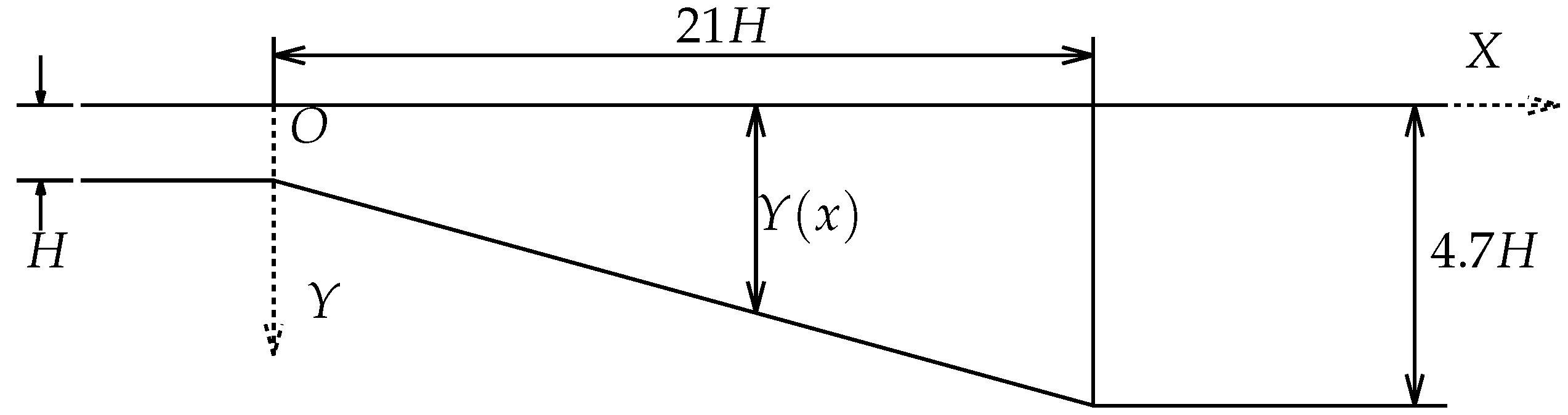
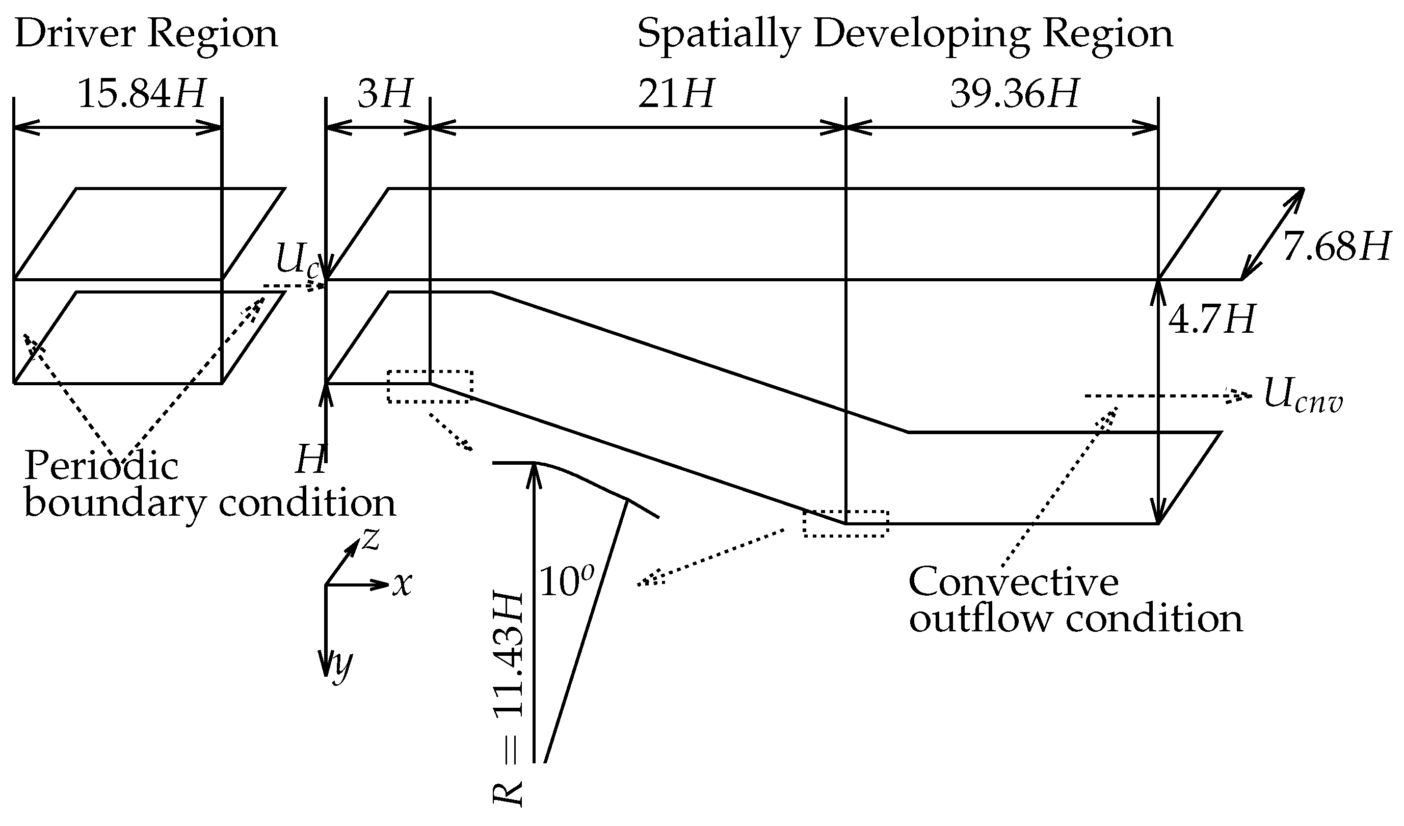
3.1. Domain Size and Boundary Condition

There are two computational regions sandwiched by two walls, called the driver and the spatially developing region, as given in Figure 2. The expansion ratio of the diffuser is 4.7 , the inclination of the wall (the lower wall) is 10 degrees and the spanwide extend is 7.68 H. The driver region length is 15.84 H and the upstream channel, expansion part and downstream extension of diffuser are 3 H, 21 H and 39.36 H, respectively. Both the joins between the expansion part and upstream/downstream parts are rounded with radius of 11.43 H, which are the same as in experiment. A Cartesian coordinate system with the origin on the upper wall where the inlet channel wall and the deflected wall form a corner is used to define x in the streamwise direction, y in the downward wall-normal direction, and z in the spanwise direction.
The flow in two regions are numerically computed simultaneously with periodic and no-slip boundary conditions for the velocity in spanwise direction and wall-normal direction, respectively. There, it should be noted that the boundary condition in the spanwise direction between simulations and the experiment performed by Obi et al. [3] is different, i.e., periodic (homogeneous) boundary condition in simulations but closed (rectangular duct) boundary condition in the experiment. To some extent, this kind of difference will affect the agreement between the simulations and the experiment, which is specifically discussed in the following. The fully-developed turbulent channel flow that is treated as inflow for the spatially-developing region are generated by the driver region with the periodic boundary condition in streamwise direction. The pressure gradients for driver region in streamwise direction are controlled to keep the flow rate a constant. Velocity profiles at outflow boundary condition for spatially-developing region are determined by a convective outflow condition
d u d t = u c n v d u d x ,
in which convective velocity u c v n is initialized with a constant bulk velocity to keep the flow rate in spatially-developing region. Finally, the pressure gradients at spatially-developing region are obtained automatically.

3.2. Computational Meshes

To assess the influence of the mesh resolution and find relatively coarser mesh for the asymmetric planar diffuser, simulations were performed on seven different collocated meshes, as given in Table 1. Here, u τ is the wall friction velocity which is found at the inlet dust, and the corresponding Reynolds number based on u τ is R e τ = 407 . In the DNS and from M1 to M5, uniform meshes are applied in the streamwise and spanwise direction for the driver and spatially-developing region, in which the mesh gradually becomes coarser from M1 to M5 in the streamwise direction while the grids remain the same in the other two directions. The nonuniform mesh are used in the streamwise direction for M6 in spatially-developing region and designed such that the spacing gradually increases from the diffuser throat toward the downstream join and the spacing gradually decreases from the inlet dust to the diffuser throat. This kind of design is necessary to resolve the sharp mean gradients in the diffuser throat for LES when the whole grids are relatively coarse. To resolve the boundary layers, the meshes in the wall normal direction distribute non-uniformly more densely near walls for all cases in both the driver and spatially-developing region. What is more, not only the boundary layers upstream but also downstream of the diffuser should be resolved in wall normal direction.

3.3. Solution Strategy

A fourth-order central finite-difference discretization scheme is used for the incompressible (filtered) continuity equation and (filtered) Navier–Stokes equation in the (LES) DNS, in which the fractional method is selected for coupling the continuity equation and the pressure field, the second-order Adams–Bashforth method is used to the convective term and viscous term, and the backward Euler method to pressure term. A fourth-order central difference schemes is applied in the Smagorinsky model. For the dynamic procedure, the test filter is used in the streamwise direction and spanwise direction with second-order accuracy and the test-to-grid filter ratio Δ ˜ / Δ = 2 . For the transport equation of the SGS kinetic energy, Crank–Nicolson method is utilized to dissipation term, the second-order Adams–Bashforth method to convective and diffusive terms. The initialization data of k s g s is solved from k s g s = ν s g s / C ν Δ ¯ 2 using the results of ν s g s from the dynamic Smagorinsky model. The present numerical method and computer program have been tested extensively in several turbulent flows [5,30,31,32].

4. Results and Discussion

All simulations were computed on an NEC SX-8R supercomputer of Cybermedia Center, Osaka University with the time step d t = 0.0495 H / U c . The great mass of the total effort of calculation was spent on solving the Poisson equation through the residual cutting method [33]. All simulations were run until the flow fields were fully developed and the first-order and second-order statistics exhibited adequate convergence. All results were collected by time averaging and spatial averaging in the spanwise direction. To allow a good comparison of simulation results and experimental measurements, the data associated with vertical cross-sections x / H = 9.2 , 15.2 , 19.2 and 25.2 in the spatially-developing region, which match the location used in previous experiments, are combined into one plot. Note that the results of our DNS for the diffuser agree quite well with the DNS results of Ohta & Kajishima [5]. For the validation discussed in this section, we restrict ourselves to use our own DNS as a comparison with three sets of LESs.

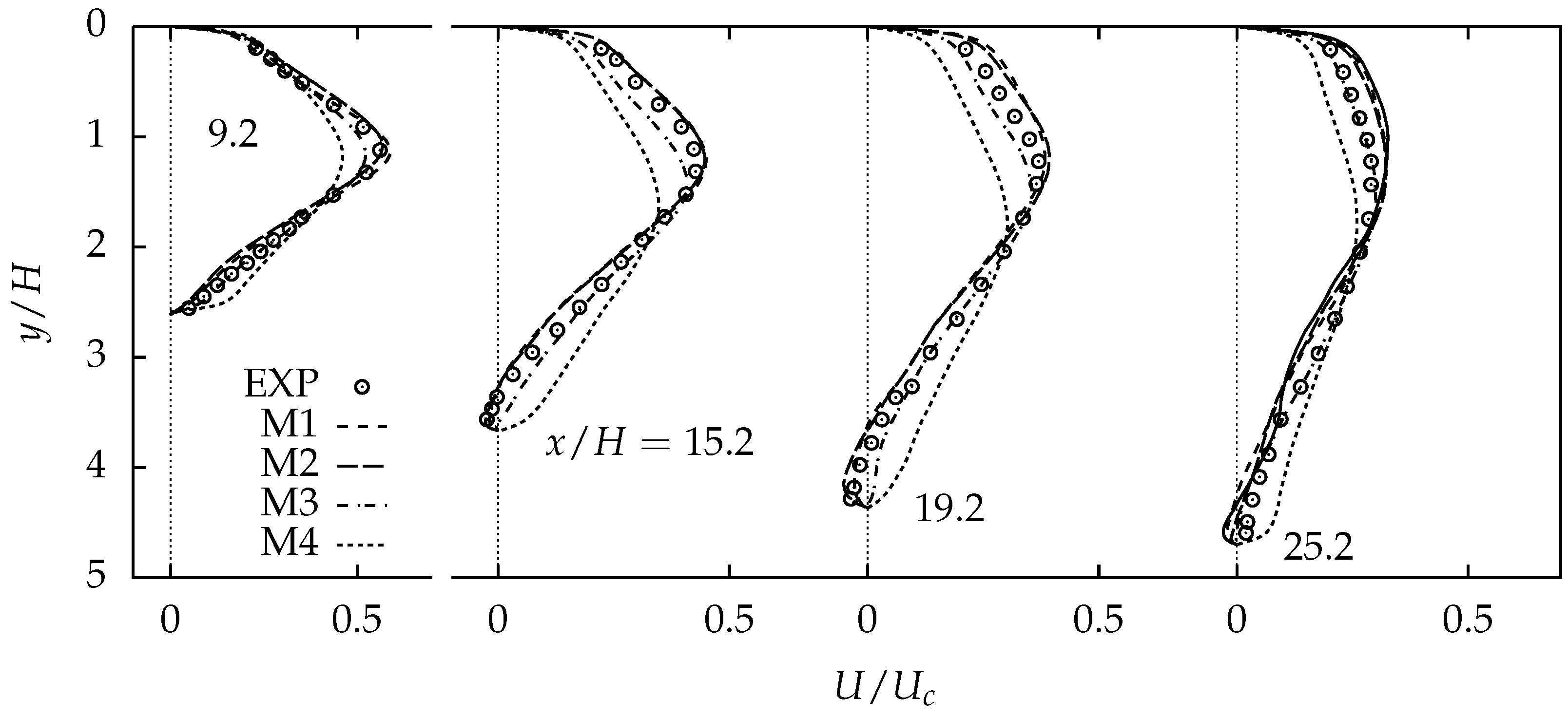
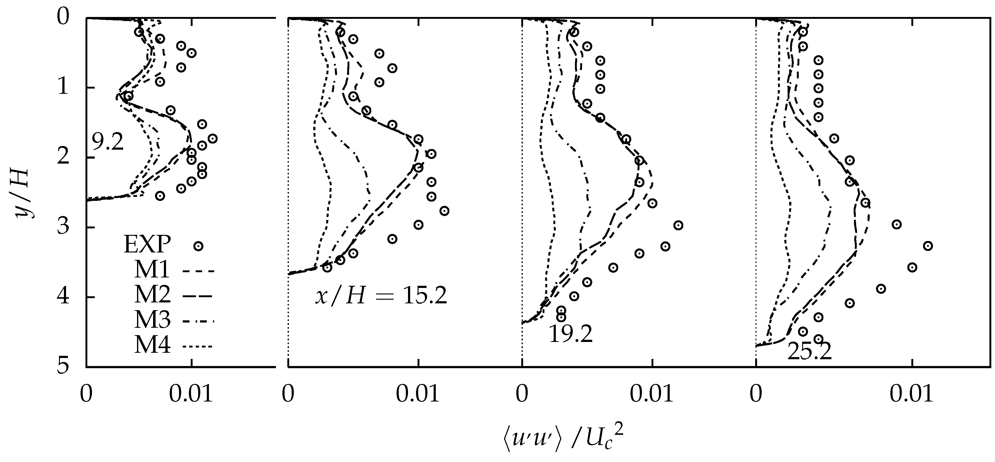
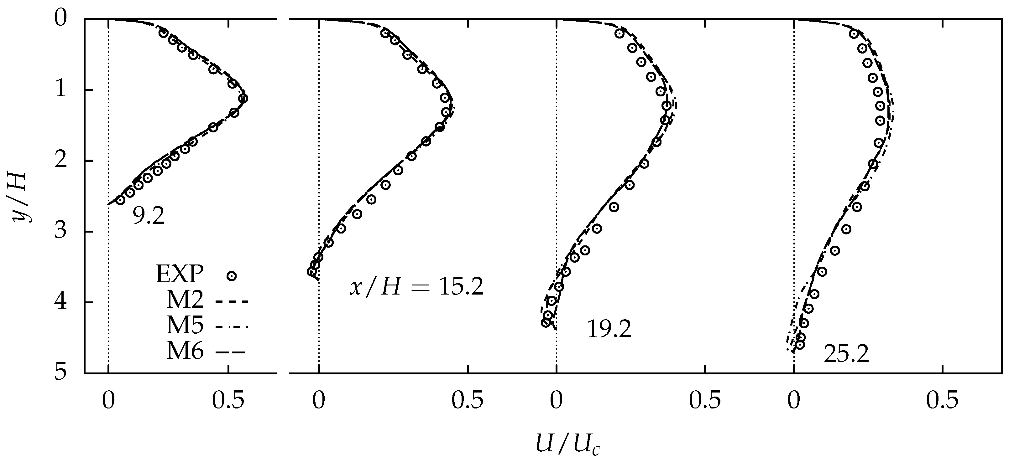
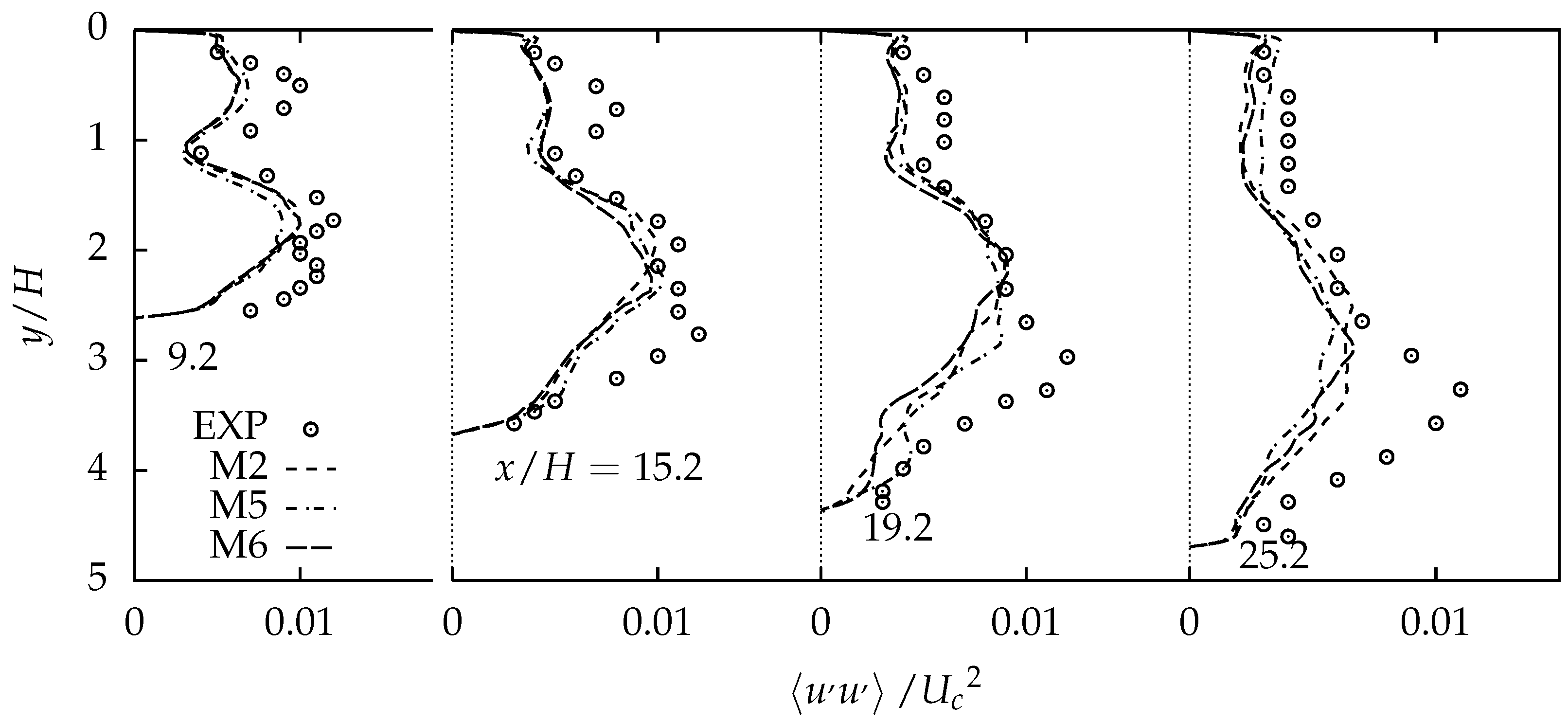
4.1. Comparison of Mesh Resolution

Figure 3, Figure 4, Figure 5 and Figure 6 show the axial mean velocity and axial Reynolds stress profiles for the mesh sensitivity study. All simulations used the LES with the standard Smagorinsky model due to its low computational cost. In Figure 3 and Figure 4, profiles of U and u u agree well with the measurement for the mesh resolution of M1 and M2, while the situation for the mesh resolution of M3 and M4 is reversed, i.e., the deviation between simulations and experiment is large. Thus, the mesh resolution of M1 and M2 rather than M3 and M4 is acceptable for the LES of the diffuser. Furthermore, differences between M1 and M2 are not apparent, although mesh of M2 is relatively coarser than M1. In Figure 4, M1 and M2 both underpredict the peak value of Reynolds stress u u and represent a large deviation in the region close to the inclined wall compared with the experimental data. Since this deviation does not decrease much with increasing mesh resolution, we suspect the standard Smagorinsky model itself and the blocking effect of the sidewall boundary layers in the experiment to contribute to this disagreement. Through the previous analysis mesh resolution of M2 and the grid spacing Δ x + = 50.38 is therefore used as a benchmark mesh and a benchmark axial grid spacing in the inlet of the diffuser, respectively. Based on the benchmark mesh and axial grid spacing, a nonuniform mesh (that is, M6) is designed and tested. In Figure 5 and Figure 6, we compare the profiles of U and u u from simulation and experiment for the different wall-normal mesh resolution and the nonuniform mesh, which shows a similar trend with M1 and M2 in Figure 3 and Figure 4. With increasing wall-normal mesh refinement from M2 and M5 an increasing agreement of the LES with the experimental data can be stated, especially in the region close to the walls, while this improvement is quite small. Even the coarsest mesh simulation, i.e., M6, demonstrates a good overall agreement with the experimental data. Thus, for the study of different SGS model performance for separating flow in the diffuser, the coarsest mesh M6 is used since the influence of the SGS model on the results is largest on this mesh.

4.2. Comparison of Subgrid Modeling

The DNS as well as five sets of LESs, i.e., SM, DSM, OM, ODM, and VOM, were computed on an NEC SX-8R supercomputer of Cybermedia Center (CMC), Osaka University. The great mass of the total effort of calculation was spent on solving the Poisson equation through the residual cutting method [33]. The time step used for these computation is about d t = 0.0495 H / U c . On a node of CMC, 13.188 s CPU time are needed to advance the computation one time step for the DNS, 1.071 s CPU time for the LES with SM model, 1.254 s CPU time for the LES with DSM model, 1.278 s CPU time for the LES with OM model, 1.391 s CPU time for the LES with ODM model, and 1.288 s CPU time for the LES with VOM model.

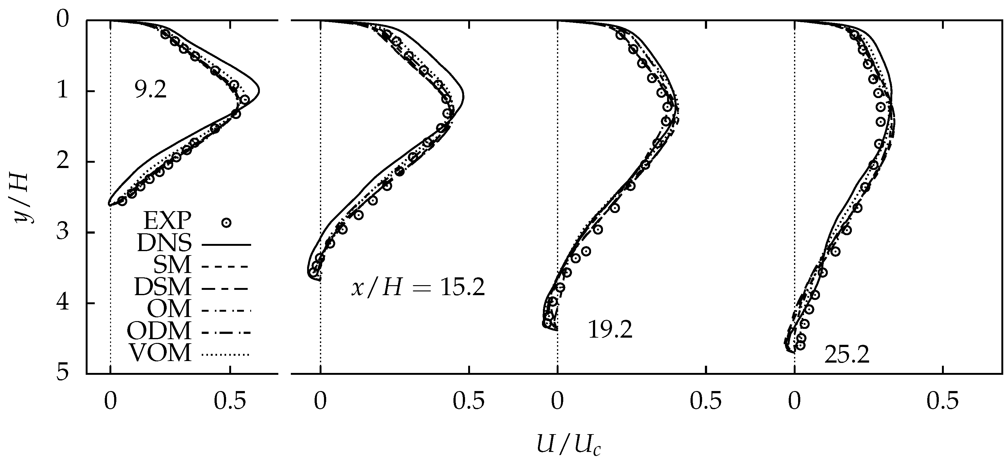
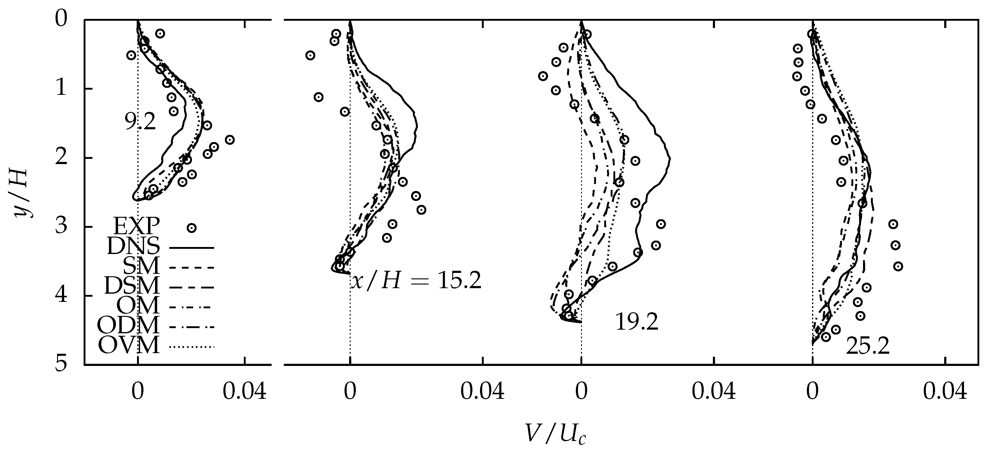
4.2.1. Comparison of Mean Properties

The profiles of the mean velocity for the streamwise direction and the wall-normal direction non-dimensionalized by the mean center velocity at the inlet duct are shown in Figure 7 and Figure 8, respectively, where five sets of LESs corresponding to the SM model, DSM model, OM model, ODM model and our OVM model are compared with DNS and experimental data of Obi. Overall, in Figure 7, the agreement of profiles of streamwise mean velocity between five LESs and experiment is quite good at all locations. The slight advance of LES velocity profile corresponding to OVM model in comparison with experimental values exists in the vicinity of the flat wall, whereas the situation adjacent to the inclined wall is reversed, i.e., the LES velocity profiles exhibit the slight lag in comparison with the measurement. This situation of velocity profiles for OVM model compared with the experiment is similar to that of DNS, but the latter exhibits more obvious difference. It seems the SM, DSM, OM and ODM models show a better overall agreement with the measurement than OVM model and DNS. Meanwhile, LESs exhibit better overall match with experiment than DNS. However, as discussed previously, agreement with the measurement is not a first priority. The results of DNS are should be used as benchmarks for SGS eddy viscosity models as well. From this perspective, the performance of OVM model in the prediction of mean streamwise velocity is slightly better than the four other SGS models since the OVM model agrees well with DNS database. Actually, the blocking effect of the sidewall boundary layers in experiment is much more pronounced for mean velocity in the wall-normal direction and turbulent stresses, which are discussed below. According to the mean velocity in the wall-normal direction from DNS and LESs, see Figure 8, the mean flow is directed from the straight (upper) wall towards the inclined wall in the flow filed except for some small regions adjacent to the inclined wall. Furthermore, the peak velocity V m a x of DNS and LESs is located in the center region of the flow filed. However, the strong flows toward the inclined wall and the straight wall are both observed in experimental data. It has been shown [34] that the influence of the side wall of the channel on the flow generated a secondary flow in the laboratory experiment, being markedly so especially in the case of a low Reynolds number. However, the agreement between simulations and measurement is good in the vicinity of the inclined wall. Compared with DNS, five SGS eddy viscosity models overpredict the mean velocity V near the diffuser throat x / H = 9.2 and underpredict V in the other regions x / H = 15.2 , 19.2 and 25.2 , except for the location at 25.2 corresponding to the DSM, ODM and OVM models. Clearly, overall, the best agreement is observed between the OVM model and DNS among five SGS eddy viscosity models.

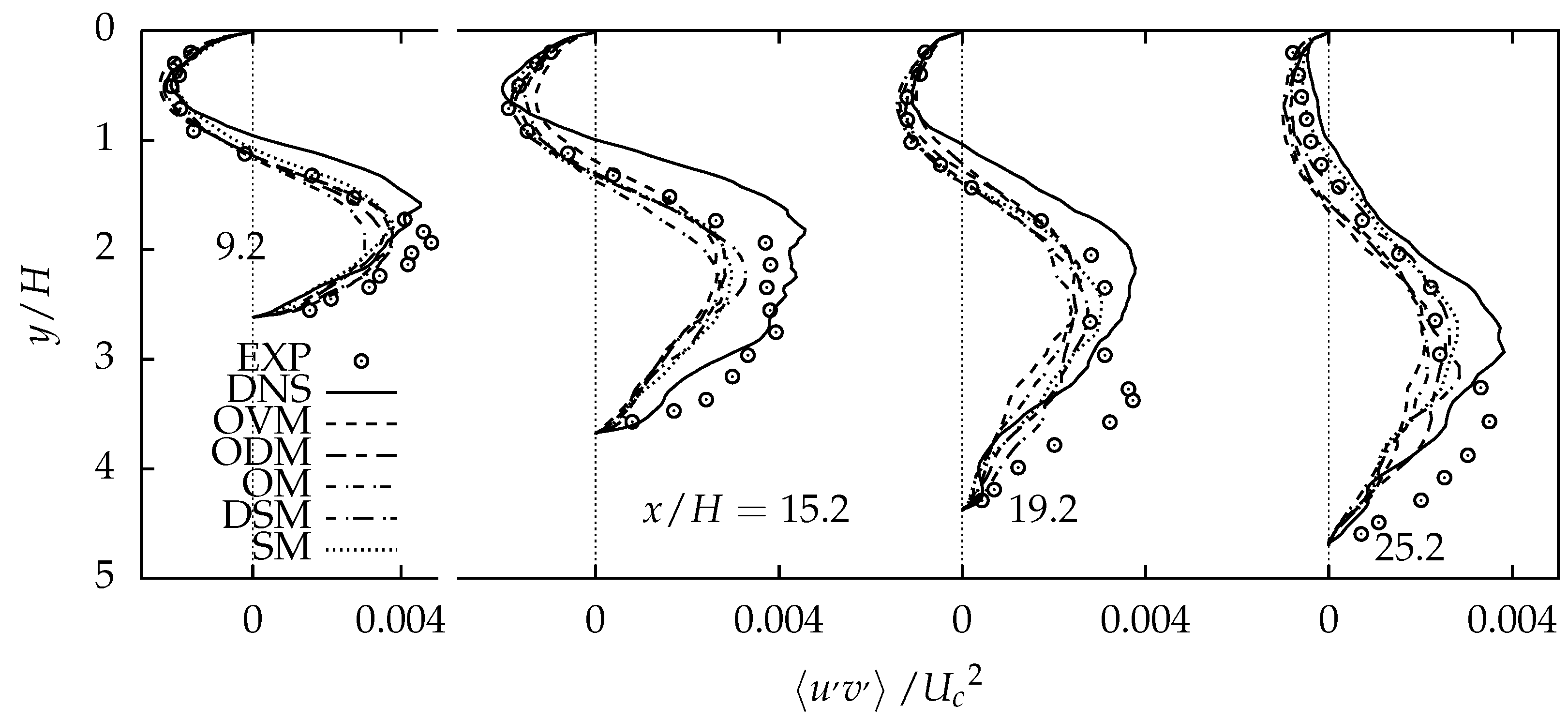
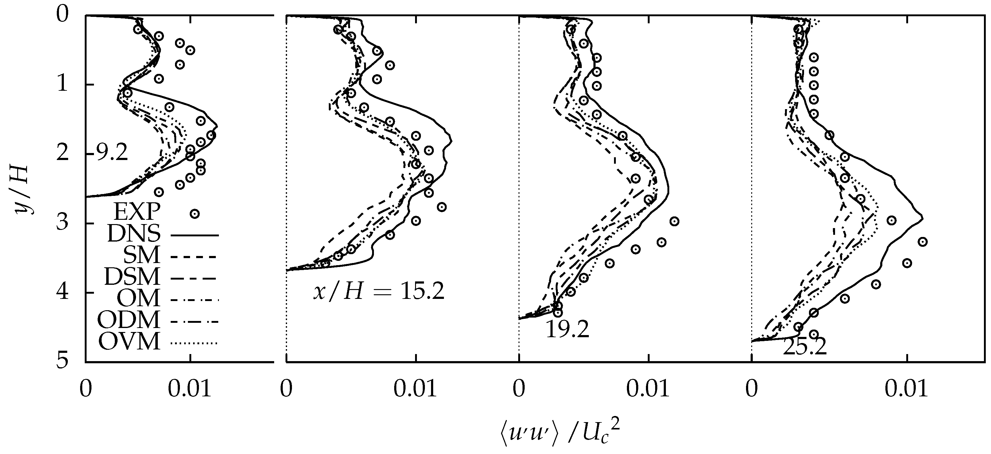
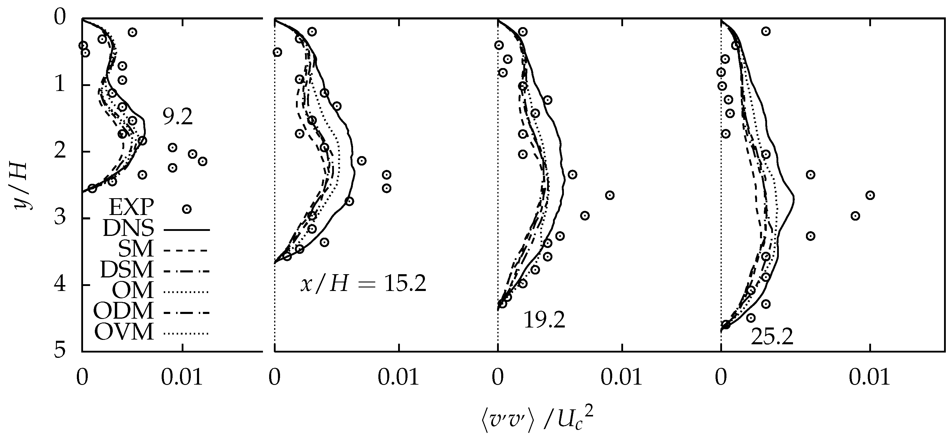
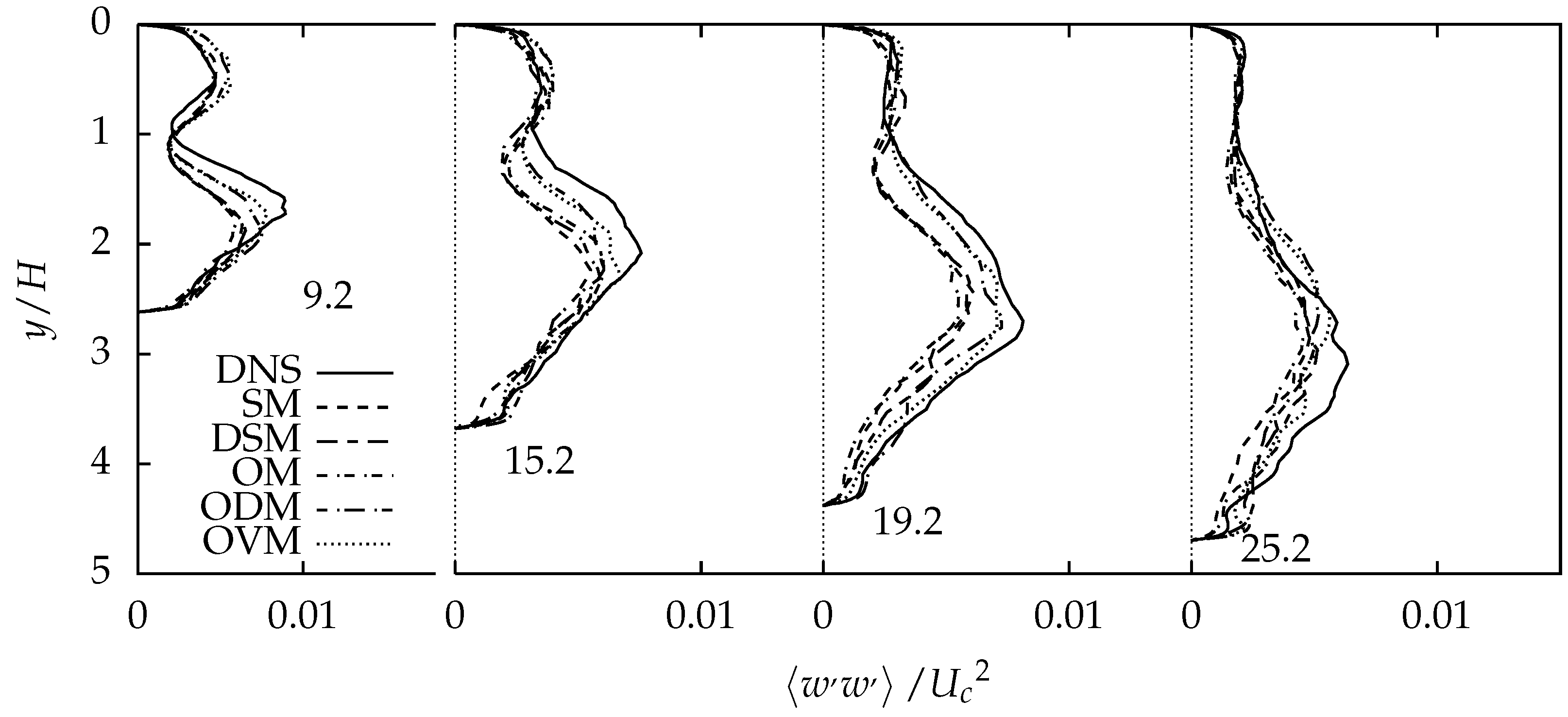
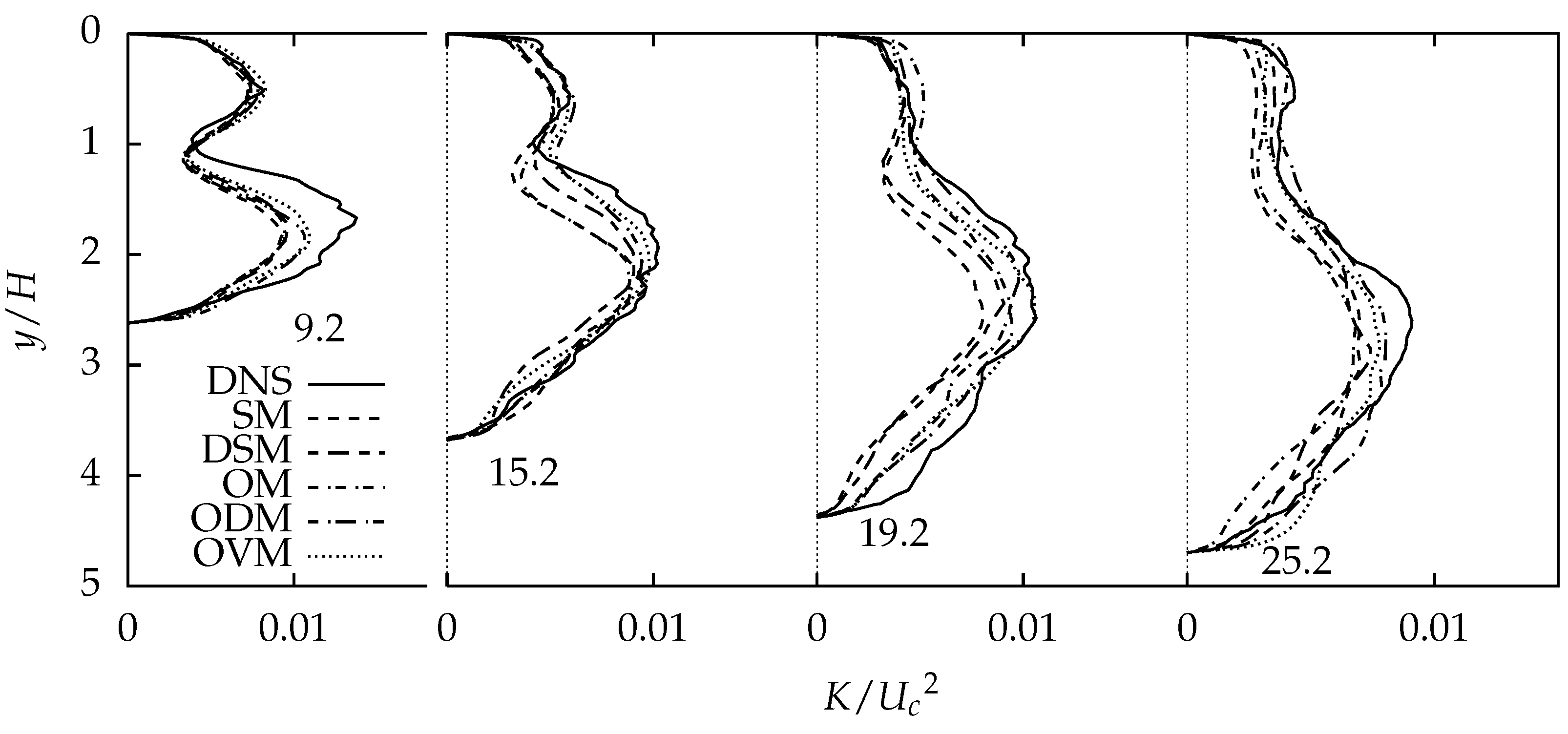
4.2.2. Comparison of Turbulent Stresses and Resolved Turbulent Kinetic Energy

In Figure 9, Figure 10, Figure 11 and Figure 12, we compare the corresponding profiles of the turbulent shear stress u v , and turbulent normal stresses u u , v v , w w from simulations and experiment, where the turbulent stresses normalized by the square of mean center velocity U c , < > refers to time averaging and spatial averaging in the homogenous direction. Note that the simulation results of three SGS eddy viscosity models are the summation of the resolvable portion and SGS portion, which coincides with the DNS and experiment. It has been shown [6] that experimental errors are higher for turbulent stresses than the mean flow velocities, in particular at the regions in which measurement volumes are large in comparison with the local gradients of turbulent stresses. However, overall, good agreement between the computations and experiment is observed at locations in the vicinity of either walls. As shown in Figure 9, turbulent shear stresses from three SGS eddy viscosity models, the DNS and experiment all exhibit a characteristic shape with a double peak. The locations of the peak value of all three SGS eddy viscosity models agree well with the DNS, whereas they are higher compared with measurement. All five SGS eddy viscosity models underpredict the peak value of turbulent shear stress compared with DNS, in which the performance of the DSM and ODM models are better than that of the SM and OM models, the OVM model demonstrates the best agreement. This can be seen especially at the location of x / H = 15.2 and 19.2 . Compared with measurement, all five SGS eddy viscosity models show a better agreement in the region close to the straight wall than the inclined wall. In the center region of the diffuser, the SM, OM, DSM and ODM models underpredict the turbulent shear stress in comparison with experiment, whereas the performance of the OVM model is a little bit of opposite. As shown in Figure 10, profiles of u u for the five SGS eddy viscosity models exhibit more prominent difference in the center region of the diffuser than adjacent to either walls, where the deviation between the SM model and the DNS or measurement is largest. Compared with the DNS as well as measurement, the SM, OM and DSM models underpredict the value of u u at all locations, except for some of small regions near the diffuser throat and further downstream. The slight advance of u u from the OVM model compared with experiment is observed in the region of flow interior. Obviously, not only the overall but also the local agreement between the OVM and ODM models and DNS / experiment is better than other three SGS eddy viscosity models. With respect to profiles of v v and w w , an overall better agreement between the LESs and the DNS is observed compared with that of turbulent shear stress and normal stress u u . A characteristic double-peak shape can still be seen for profiles in Figure 11 and Figure 12. The location of the peak value moves away from the wall into the flow interior with increasing distance from the diffuser throat. While the peak value of the turbulent stress v v from DNS as well as LESs gravely deviates from the measurement, locations of the peak value are close to each other and coincide with the measurement, except for the location at x / H = 9.2 . In comparison with the DNS, SM model, DSM model, OM model and ODM model underpredict v v and w w at all locations, except for some of small regions adjacent to straight wall, whereas the OVM model slightly overpredicts both of them in the vicinity of the inclined wall. Overall, the OVM model agree better with the DNS than other four SGS eddy viscosity models. Figure 13 shows the profiles of the resolved turbulent kinetic energy K non-dimensionalized by the square of the mean center velocity. All five SGS eddy viscosity models capture the locations as well as the magnitude of the double-peak in K. Compared with the DNS, the five SGS models accurately predict the near-wall peak of the straight wall except for the location at x / H = 25.2 , but underpredict the larger peak value at all location. In particular, the SM model and the OM model do not correctly capture the location of the larger peak for the locations at x / H = 15.2 . The OVM model agrees well with the DNS with respect to the location as well as the value of the double-peak in the resolved turbulent kinetic energy.

5. Conclusions

The turbulent flow through a planar asymmetric diffuser was investigated numerically using LES with a high-order finite difference method to solve the equations for the resolved scales. Six resolutions were conducted for investigating the influence of mesh resolution in the turbulent diffuser flow. Four existing SGS models, a new one-equation dynamic model and a DNS were performed for LES of turbulent diffuser flow. The performance of five different SGS models was compared with published experiments and our DNS results. Firstly, LES on a coarse grid using the standard Smagorinsky model and well-designed wall-functions is able to predict the three-dimensional separated diffuser flow with fair accuracy at reasonable cost. Secondly, the ODM model and OVM model gave better agreement with experiments and DNS than the SM model, OM model and DSM model. Thirdly, unlike the ODM model, our OVM model, which does not require any test filtering and is not more expensive in terms of computational cost than the standard one-equation model, gave considerable improvement of the prediction accuracy even with moderate grid resolution in comparison with the four other SGS models.

Author Contributions

H.T. and Y.L. conceived the original ideal; H.T. wrote and edited the manuscript; and Y.L., X.L. and Y.F. supervised the study.

Funding

This research was funded by the project of Chinese National Natural Science Foundation (grant number: 51575220), the project of the Key Scientific and Technological Project of Jilin Province (grant numbers: 20160519008JH and 20170204073GX), and the project of National Key R&D Program of China (grant number: 2016YFB0101402).

Acknowledgments

The authors thank Takeo Kajishima and Kei Okabayashi for their help with the numerical method proposed and simulations conducted.

Conflicts of Interest

The authors declare no conflict of interest.

Abbreviations

The following abbreviations are used in this manuscript:
CFDComputational fluid dynamics
DNSDirect numerical simulation
DSMStandard dynamic Smagorinsky model
LESLarge eddy simulation
N-SNavier–Stokes
ODMOne-equation dynamic model
OMStandard one-equation model
OVMOne-equation Vreman model
RANSReynolds-averaged Navier–Stokes simulation
SGSsubgrid scale
SMSmagorinsky model

Appendix A. Determination of the Distance from the Wall Measured in Wall Units in the Diffuser Flow for Smagorinsky Model

Using a linear interpolation, let us assume the friction velocity u τ ( x ) in the diffuser is as follows:
u τ ( x ) = u τ 0 , x 0 u τ 0 + x ( u τ e u τ 0 ) / H , 0 < x 21 H u τ e , x > 21 H ,
where u τ 0 denotes the inlet friction velocity, 407; and u τ e denotes the friction velocity in down stream extension.
Reynolds number R e m based on the bulk velocity U m is constant in the diffuser because of the continuity:
U m H ν = U m 4.7 4.7 H ν .
Thus, R e τ is also constant due to the Dean’s suggested correction [35] R e τ = 0.191 R e m 0.875 , which was validated by Kim et al. [4] in fully developed channel flow. Then, R e τ in diffuser can be approximately expressed as:
R e τ 0 = u τ 0 · H ν = u τ e · 4.7 H ν = 407 ,
thus we get u τ e = u τ 0 / 4.7 . Using Equation (A1), y + can be approximately defined as:
y + ( x , y ) = R e τ 0 · min ( y , 1 y ) / H , x 0 R e τ 0 · ( 1 3.7 / 4.7 · x / H ) · min [ y , Y ( x ) y ] / H , 0 < x 21 H R e τ 0 / 4.7 · min ( y , 4.7 H y ) / H , x > 21 H .

References

  1. Sayles, E.L.; Eaton, J.K. Sensitivity of an asymmetric, three-dimensional diffuser to inlet condition perturbations. Int. J. Heat Fluid Flow 2014, 49, 100–107. [Google Scholar] [CrossRef]
  2. Azad, R.S. Turbulent flow in a conical diffuser: A review. Exp. Fluid Sci. 1996, 13, 318–337. [Google Scholar] [CrossRef]
  3. Obi, S.; Aoki, K.; Masuda, S. Experimental and computational study of turbulent separating flow in an asymmetric plane diffuser. In Proceedings of the Ninth Symposium on Turbulent Shear Flows, Hyoto, Japan, 16–18 August 1993; p. 305-1. [Google Scholar]
  4. Kim, J.; Moin, P.; Moser, R. Turbulence statistics in fully developed channel flow at low Reynolds number. J. Fluid Mech. 1987, 177, 133–166. [Google Scholar] [CrossRef] [Green Version]
  5. Ohta, T.; Kajishima, T. Analysis of non-steady separated turbulent flow in an asymmetric plane diffuser by direct numerical simulations. J. Fluid Sci. Technol. 2010, 5, 515–527. [Google Scholar] [CrossRef]
  6. Kaltenbach, H.J.; Fatica, M.; Mittal, R.; Lund, T.S.; Moin, P. Study of flow in a planar asymmetric diffuser using large-eddy simulation. J. Fluid Mech. 1999, 390, 151–185. [Google Scholar] [CrossRef]
  7. Durbin, P.A. Separated flow computations with the k-epsilon-v-squared model. AIAA J. 1995, 33, 659–664. [Google Scholar] [CrossRef]
  8. Iaccarino, G. Predictions of a turbulent separated flow using commercial CFD codes. J. Fluids Eng. 2001, 123, 819–828. [Google Scholar] [CrossRef]
  9. El-Behery, S.M.; Hamed, M.H. A comparative study of turbulence models performance for separating flow in a planar asymmetric diffuser. Comput. Fluids 2011, 44, 248–257. [Google Scholar] [CrossRef]
  10. Schneider, H.; von Terzi, D.; Bauer, H.J.; Rodi, W. Reliable and accurate prediction of three-dimensional separation in asymmetric diffusers using large-eddy simulation. J. Fluids Eng. 2010, 132, 031101. [Google Scholar] [CrossRef]
  11. Abe, K.I.; Ohtsuka, T. An investigation of LES and Hybrid LES/RANS models for predicting 3-D diffuser flow. Int. J. Heat Fluid Flow 2010, 31, 833–844. [Google Scholar] [CrossRef]
  12. Schluter, J.; Wu, X.; Pitsch, H. Large-Eddy Ssimulations of a Separated Plane Diffuser. In Proceedings of the 43rd AIAA Aerospace Sciences Meeting and Exhibit, Reno, NV, USA, 10–13 January 2005; p. 672. [Google Scholar]
  13. Kobayashi, H.; Ham, F.; Wu, X. Application of a local SGS model based on coherent structures to complex geometries. Int. J. Heat Fluid Flow 2008, 29, 640–653. [Google Scholar] [CrossRef]
  14. Taghinia, J.; Rahman, M.M.; Siikonen, T.; Agarwal, R.K. One-equation sub-grid scale model with variable eddy-viscosity coefficient. Comput. Fluids 2015, 107, 155–164. [Google Scholar] [CrossRef]
  15. Shuai, S.; Agarwal, R.K. A One-Equation Turbulence Model Based on k-kL Closure. In Proceedings of the AIAA Scitech 2019 Forum, San Diego, CA, USA, 7–11 January 2019; p. 1879. [Google Scholar]
  16. Sagaut, P. Large Eddy Simulation for Incompressible Flows: An Introduction; Springer Science & Business Media: Berlin/Heidelberg, Geramny, 2006. [Google Scholar]
  17. Smagorinsky, J. General circulation experiments with the primitive equations: I. The basic experiment. Mon. Weather Rev. 1963, 91, 99–164. [Google Scholar] [CrossRef]
  18. Germano, M.; Piomelli, U.; Moin, P.; Cabot, W.H. A dynamic subgrid-scale eddy viscosity model. Phys. Fluids A 1991, 3, 1760–1765. [Google Scholar] [CrossRef]
  19. Lilly, D.K. A proposed modification of the Germano subgrid-scale closure method. Phys. Fluids A 1992, 4, 633–635. [Google Scholar] [CrossRef]
  20. Yoshizawa, A. A statistically-derived subgrid model for the large-eddy simulation of turbulence. Phys. Fluids 1982, 25, 1532–1538. [Google Scholar] [CrossRef]
  21. Kajishima, T.; Nomachi, T. One-equation subgrid scale model using dynamic procedure for the energy production. J. Appl. Mech. 2006, 73, 368–373. [Google Scholar] [CrossRef]
  22. Yoshizawa, A.; Horiuti, K. A statistically-derived subgrid-scale kinetic energy model for the large-eddy simulation of turbulent flows. J. Phys. Soc. Jpn. 1985, 54, 2834–2839. [Google Scholar] [CrossRef]
  23. Horiuti, K. Large eddy simulation of turbulent channel flow by one-equation modeling. J. Phys. Soc. Jpn. 1985, 54, 2855–2865. [Google Scholar] [CrossRef]
  24. Okamoto, M.; Shima, N. Investigation for the One-Eaquation-Type Subgrid Model with Eddy-Viscosity Expression Including the Shear-Damping Effect. JSME Int. J. Ser. B 1999, 42, 154–161. [Google Scholar] [CrossRef]
  25. Vreman, A.W. An eddy-viscosity subgrid-scale model for turbulent shear flow: Algebraic theory and applications. Phys. Fluids 2004, 16, 3670–3681. [Google Scholar] [CrossRef]
  26. Park, N.; Lee, S.; Lee, J.; Choi, H. A dynamic subgrid-scale eddy viscosity model with a global model coefficient. Phys. Fluids 2006, 18, 125109. [Google Scholar] [CrossRef]
  27. You, D.; Moin, P. A dynamic global-coefficient subgrid-scale eddy-viscosity model for large-eddy simulation in complex geometries. Phys. Fluids 2007, 19, 065110. [Google Scholar] [CrossRef] [Green Version]
  28. You, D.; Moin, P. A dynamic global-coefficient subgrid-scale model for large-eddy simulation of turbulent scalar transport in complex geometries. Phys. Fluids 2009, 21, 045109. [Google Scholar] [CrossRef] [Green Version]
  29. Obi, S.; Ohizumi, H.; Aoki, K.; Masuda, S. Turbulent separation control in a plane asymmetric diffuser by periodic perturbation. Eng. Turbul. Model. Exp. 1993, 633–642. [Google Scholar] [CrossRef]
  30. Kajishima, T.; Ohta, T.; Okazaki, K.; Miyake, Y. High-order finite-difference method for incompressible flows using collocated grid system. JSME Int. J. Ser. B 1998, 41, 830–839. [Google Scholar] [CrossRef]
  31. Ohta, T. DNS of turbulent channel flow subjected to the acceleration. Trans. Jpn. Soc. Mech. Eng. Ser. B 2004, 70, 1–8. [Google Scholar] [CrossRef]
  32. Tang, H.; Lei, Y.; Fu, Y. Noise Reduction Mechanisms of an Airfoil with Trailing Edge Serrations at Low Mach Number. Appl. Sci. 2019, 9, 3784. [Google Scholar] [CrossRef]
  33. Tamura, A.; Kikuchi, K.; Takahashi, T. Residual cutting method for elliptic boundary value problems. J. Comput. Phys. 1997, 137, 247–264. [Google Scholar] [CrossRef]
  34. Buice, C.U.; Eaton, J.K. Experimental Investigation of Flow Through an Asymmetric Plane Diffuser. Center for Turbulence Research Annual Research Briefs 1995, 117–120. [Google Scholar] [CrossRef]
  35. Dean, R.B. Reynolds number dependence of skin friction and other bulk flow variables in two-dimensional rectangular duct flow. J. Fluids Eng. 1978, 100, 215–223. [Google Scholar] [CrossRef]
Figure 1. Schematic of an asymmetric plane diffuser.
Symmetry 11 01337 g001
Figure 2. Three-dimensional schematic of Obi et al. diffuser.
Symmetry 11 01337 g002
Figure 3. Comparison of LES with different mesh resolution in the streamwise direction and experimental results of Obi in terms of mean streamwise velocity profiles.
Symmetry 11 01337 g003
Figure 4. Comparison of LES with different mesh resolution in streamwise direction and experimental results of Obi in terms of axial Reynolds stress profiles.
Symmetry 11 01337 g004
Figure 5. Comparison of LES with different mesh resolution and experimental results of Obi in terms of axial mean velocity profiles.
Symmetry 11 01337 g005
Figure 6. Comparison of LES with different mesh resolution and experimental results of Obi in terms of axial Reynolds stress profiles.
Symmetry 11 01337 g006
Figure 7. Comparison of LES with different SGS models, DNS and experimental results of Obi in terms of axial mean velocity profiles.
Symmetry 11 01337 g007
Figure 8. Comparison of LES with different SGS models, DNS and experimental results of Obi in terms of wall-normal mean velocity profiles.
Symmetry 11 01337 g008
Figure 9. Comparison of LES with different SGS models, DNS and experimental results of Obi in terms of Reynolds shear stress profiles.
Symmetry 11 01337 g009
Figure 10. Comparison of LES with different SGS models, DNS and experimental results of Obi in terms of Reynolds stress u u / U c 2 profiles.
Symmetry 11 01337 g010
Figure 11. Comparison of LES with different SGS models, DNS and experimental results of Obi in terms of Reynolds stress v v / U c 2 profiles.
Symmetry 11 01337 g011
Figure 12. Comparison of LES with different SGS models, DNS and experimental results of Obi in terms of Reynolds stress w w / U c 2 profiles.
Symmetry 11 01337 g012
Figure 13. Comparison of LES with different SGS models, DNS and experimental results of Obi in terms of resolved turbulent kinetic energy profiles.
Symmetry 11 01337 g013
Table 1. Mesh resolution of simulations: N x , N y , and N z denote the number of cells in streamwise, wall-normal and spanwise direction, respectively. Δ x + , Δ y + , and Δ z + are grid spacing used in simulations normalized by ν / u τ . Super/subscripts of 1 and 2 represent driver and spatially-developing region, respectively.
Case N x 1 N x 2 N y N z Δ x 1 + Δ x 2 + Δ y min + Δ z +
DNS320120016032020.1520.150.509.77
M11606008016040.3040.301.0419.54
M21284808016050.3850.381.0419.54
M31283608016050.3867.171.0419.54
M41283008016050.3880.61.0419.54
M512848016016050.3850.380.5019.54
M61283728016050.3850.38–100.761.0419.54

