The Cauchy Conjugate Gradient Algorithm with Random Fourier Features


Abstract
:1. Introduction
2. Background
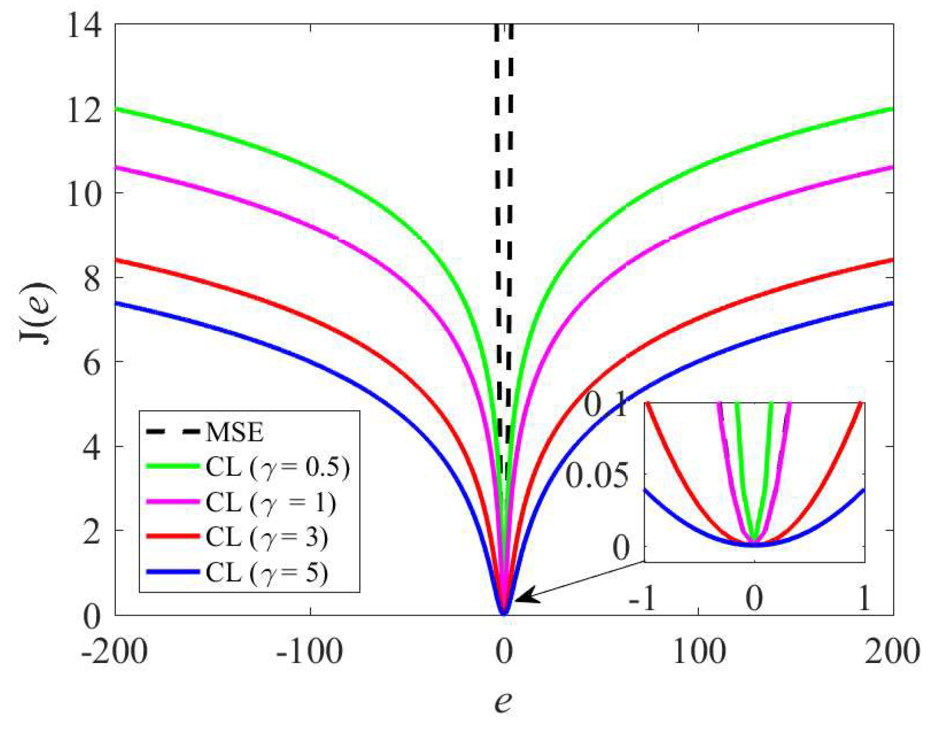
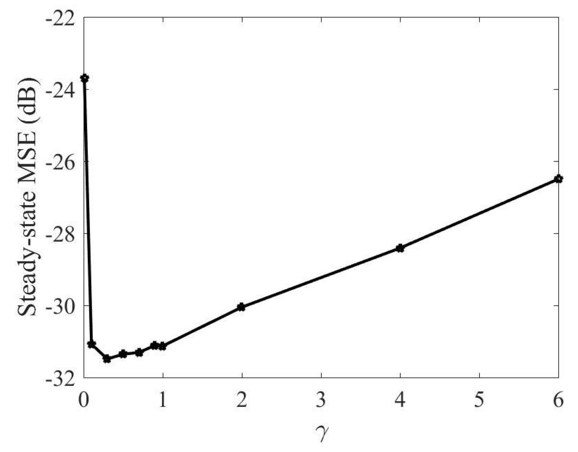
2.1. Minimum Cauchy Loss Criterion
2.2. Conjugate Gradient Algorithm
2.3. Online Conjugate Gradient Algorithm
3. Proposed Algorithm
3.1. Random Fourier Mapping
3.2. RFFCCG Algorithm
| Algorithm 1: The robust random Fourier features Cauchy conjugate gradient (RFFCCG) algorithm. |
| Input: Sequential input–output pairs , kernel bandwidth , forgetting factor , the dimension of RFF , and constant . Draw: i.i.d. , where the dimension of original data space . i.i.d. , where U denotes the uniform distribution. Initialization: , , , , , , , . Computation: while { is available, do 1. , 2. , 3. , 4. , 5. , 6. , 7. , 8. , 9. , 10. . end while |
3.3. Complexity
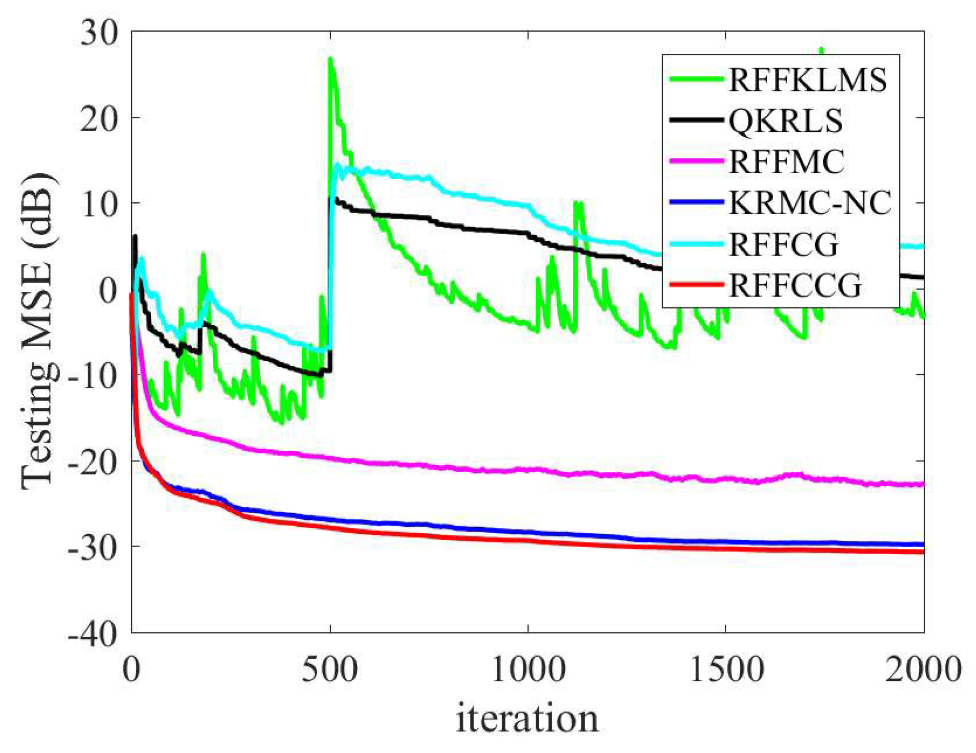
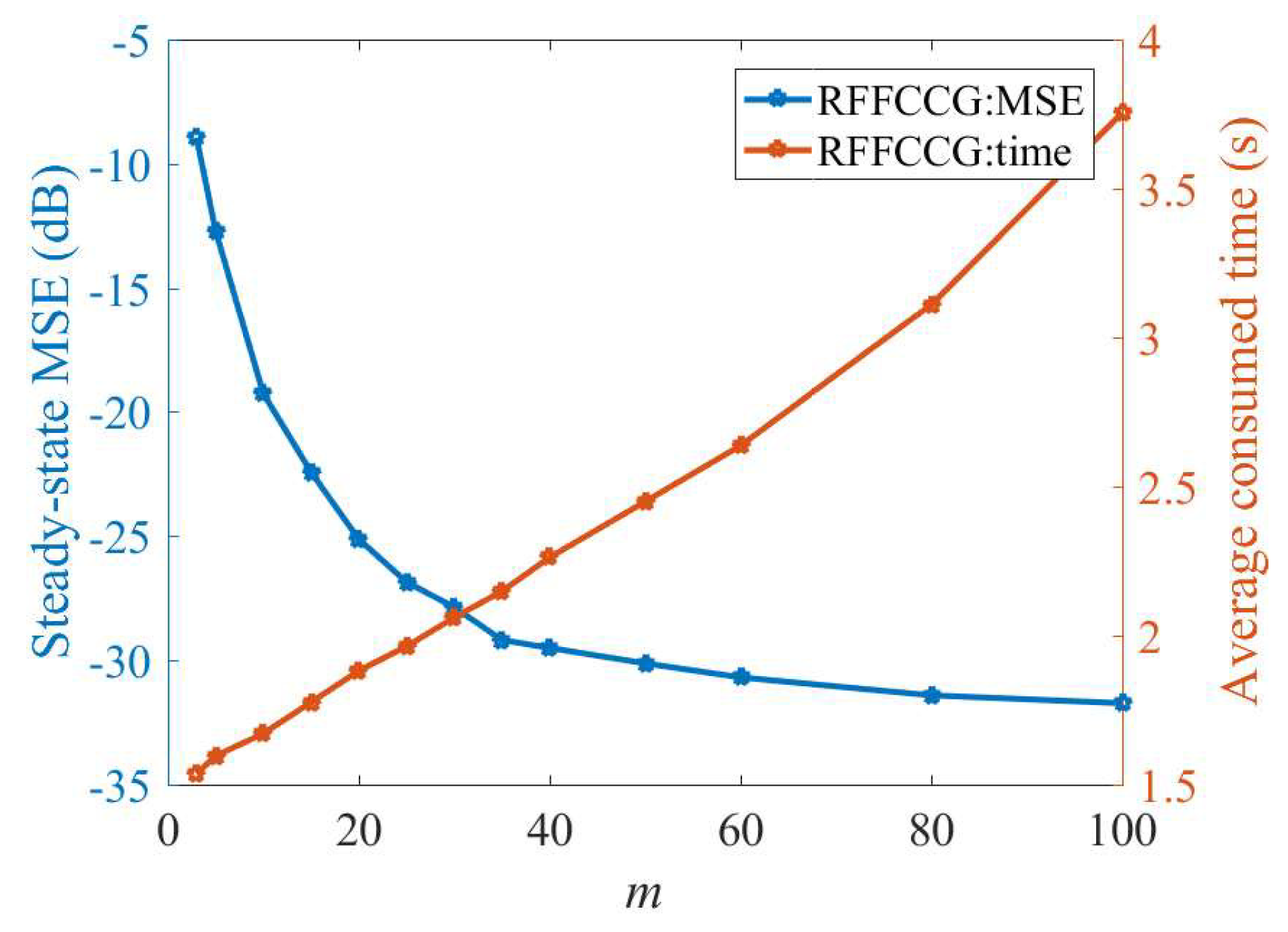
4. Simulation
4.1. Mackey–Glass Time Series
4.2. Nonlinear System Identification
5. Conclusions
Author Contributions
Funding
Conflicts of Interest
References
- Kivinen, J.; Smola, A.J.; Williamson, R.C. Online learning with kernels. IEEE Trans. Signal Process. 2004, 52, 1540–1547. [Google Scholar] [CrossRef]
- Liu, W.; Príncipe, J.C.; Haykin, S. Kernel Adaptive Filtering: A Comprehensive Introduction; John Wiley & Sons: Hoboken, NJ, USA, 2010. [Google Scholar]
- Liu, W.; Pokharel, P.P.; Príncipe, J.C. The kernel least mean square algorithm. IEEE Trans. Signal Process. 2008, 56, 543–554. [Google Scholar] [CrossRef]
- Liu, W.; Príncipe, J.C. Kernel affine projection algorithms. EURASIP J. Adv. Signal Process. 2008, 2008, 1–12. [Google Scholar]
- Engel, Y.; Mannor, S.; Meir, R. The kernel recursive least squares algorithm. IEEE Trans. Signal Process. 2004, 52, 2275–2285. [Google Scholar] [CrossRef]
- Liu, W.; Park, I.; Príncipe, J.C. An information theoretic approach of designing sparse kernel adaptive filters. IEEE Trans. Neural Netw. 2009, 20, 1950–1961. [Google Scholar] [CrossRef]
- Richard, C.; Bermudez, J.C.M.; Honeine, P. Online prediction of time series data with kernels. IEEE Trans. Signal Process. 2009, 57, 1058–1067. [Google Scholar] [CrossRef]
- Wang, S.; Zheng, Y.; Duan, S.; Wang, L.; Tan, T. Quantized kernel maximum correntropy and its mean square convergence analysis. Dig. Signal Process. 2017, 63, 164–176. [Google Scholar] [CrossRef]
- Zhao, S.; Chen, B.; Zhu, P.; Príncipe, J.C. Fixed budget quantized kernel least mean square algorithm. Signal Process. 2013, 93, 2759–2770. [Google Scholar] [CrossRef]
- Vaerenbergh, S.V.; Vía, J.; Santamaría, I. A sliding-window kernel RLS algorithm and its application to nonlinear channel identification. In Proceedings of the 2006 IEEE International Conference on Acoustics Speech and Signal Processing Proceedings (ICASSP), Toulouse, France, 14–19 May 2006; pp. 789–792. [Google Scholar]
- Wang, S.; Wang, W.; Dang, L.; Jiang, Y. Kernel least mean square based on the Nyström method. Circuits Syst. Signal Process. 2019, 38, 3133–3151. [Google Scholar] [CrossRef]
- Rahimi, A.; Recht, B. Random features for large-scale kernel machines. In Proceedings of the 21th Annual Conference on Neural Information Processing Systems (ACNIPS), Vancouver, BC, Canada, 3–6 December 2007; pp. 1177–1184. [Google Scholar]
- Singh, A.; Ahuja, N.; Moulin, P. Online learning with kernels: Overcoming the growing sum problem. In Proceedings of the 2012 IEEE International Workshop on Machine Learning for Signal Process (MLSP), Santander, Spain, 23–26 September 2012; pp. 1–6. [Google Scholar]
- Wang, S.; Dang, L.; Chen, B.; Duan, S.; Wang, L.; Tse, C.K. Random Fourier filters under maximum correntropy criterion. IEEE Trans. Circuits Syst. I Reg. Pap. 2018, 65, 3390–3403. [Google Scholar] [CrossRef]
- Xiong, K.; Wang, S. The online random Fourier features conjugate gradient algorithm. IEEE Signal Process. Lett. 2019, 26, 740–744. [Google Scholar] [CrossRef]
- Wu, Q.; Li, Y.; Xue, W. A kernel recursive maximum versoria-like criterion algorithm for nonlinear channel equalization. Symmetry 2019, 11, 1067. [Google Scholar] [CrossRef]
- Mathews, V.J.; Cho, S.H. Improved convergence analysis of stochastic gradient adaptive filters using the sign algorithm. IEEE Trans. Acoust. Speech Signal Process. 1987, 35, 450–454. [Google Scholar] [CrossRef]
- Walach, E.; Widrow, B. The least mean fourth (LMF) adaptive algorithm and its family. IEEE Trans. Inf. Theory 1984, 42, 275–283. [Google Scholar] [CrossRef]
- Príncipe, J.C. Information Theoretic Learning: Renyi’s Entropy and Kernel Perspectives; Springer: New York, NY, USA, 2010. [Google Scholar]
- Li, Y.; Wang, Y.; Sun, L. A proportionate normalized maximum correntropy criterion algorithm with correntropy induced metric constraint for identifying sparse systems. Symmetry 2018, 10, 683. [Google Scholar] [CrossRef]
- Gallagher, C.H.; Fisher, T.J.; Shen, J. A cauchy estimator test for autocorrelation. J. Stat. Comput. Simul. 2015, 85, 1264–1276. [Google Scholar] [CrossRef]
- Luenberger, D.G. Linear and Nonlinear Programming, 4th ed.; Prentice Hall: Englewood Cliffs, NJ, USA, 2016. [Google Scholar]
- Yang, J.; Ye, F.; Rong, H.J.; Chen, B. Recursive least mean p-Power extreme learning machine. Neural Netw. 2017, 91, 22–33. [Google Scholar] [CrossRef]
- Boray, G.K.; Srinath, M.D. Conjugate gradient techniques for adaptive filtering. IEEE Trans. Circuits Syst. I Fundam. Theory Appl. 1992, 39, 1–10. [Google Scholar] [CrossRef]
- Chang, P.S.; Willson, A.N. Analysis of conjugate gradient algorithms for adaptive filtering. IEEE Trans. Signal Process. 2008, 48, 409–418. [Google Scholar] [CrossRef]
- Hestenes, M.R.; Stiefel, E. Methods of conjugate gradients for solving linear systems. J. Res. Nat. Bur. Stand. 1952, 49, 409–436. [Google Scholar] [CrossRef]
- Dassios, I.; Fountoulakis, K.; Gondzio, J. A preconditioner for a primal-dual newton conjugate gradients method for compressed sensing problems. SIAM J. Sci. Comput. 2015, 37, 2783–2812. [Google Scholar] [CrossRef]
- Heravi, A.R.; Hodtani, G.A. A new correntropy-based conjugate gradient backpropagation algorithm for improving training in neural networks. IEEE Trans. Neural Netw. Learn. Syst. 2018, 29, 6252–6263. [Google Scholar] [CrossRef] [PubMed]
- Caliciotti, A.; Fasano, G.; Roma, M. Preconditioned nonlinear conjugate gradient methods based on a modified secant equation. Appl. Math. Comput. 2018, 318, 196–214. [Google Scholar] [CrossRef]
- Zhang, M.; Wang, X.; Chen, X.; Zhang, A. The kernel conjugate gradient algorithms. Trans. Signal Process. 2018, 66, 4377–4387. [Google Scholar] [CrossRef]
- Wu, Z.; Shi, J.; Zhang, X.; Ma, W.; Chen, B. Kernel recursive maximum correntropy. Signal Process. 2015, 117, 11–16. [Google Scholar] [CrossRef]
- Chen, B.; Zhao, S.; Zhu, P.; Príncipe, J.C. Quantized kernel recursive least squares algorithm. IEEE Trans. Neural Netw. Learn. Syst. 2013, 24, 1484–1491. [Google Scholar] [CrossRef]
- Chen, B.; Xing, L.; Zhao, H.; Zheng, N.; Príncipe, J.C. Generalized correntropy for robust adaptive filtering. IEEE Trans. Signal Process. 2016, 64, 3376–3387. [Google Scholar] [CrossRef]
- Weng, B.; Barner, K.E. Nonlinear system identification in impulsive environments. IEEE Trans. Signal Process. 2005, 53, 2588–2594. [Google Scholar] [CrossRef]
- Chen, S.; Billings, S.A.; Grant, P.M. Recursive hybrid algorithm for non-linear system identification using radial basis function networks. Int. J. Control 1992, 55, 1051–1070. [Google Scholar] [CrossRef]


| Algorithm | Addition | Multiplication | Division |
|---|---|---|---|
| 1-4KLMS [3] | k | k | 0 |
| KRLS [5] | 1 | ||
| KRMC [31] | 2 | ||
| KCG [30] | 3 | ||
| RFFCCG | 4 |
| Algorithm | Matrix | ||
|---|---|---|---|
| KLMS [3] | 0 | 1 | 0 |
| KRLS [5] | 0 | 1 | 1 |
| KRMC [31] | 0 | 1 | 1 |
| KCG [30] | 0 | 1 | 1 |
| RFFCCG | 1 | 0 | 0 |
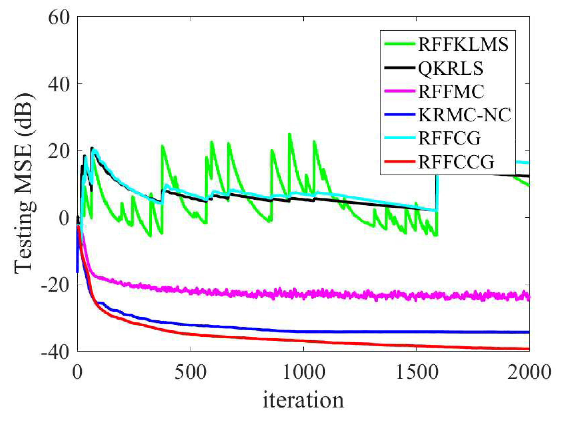
| Algorithm | Size | MSE | Consumed Time |
|---|---|---|---|
| RFFKLMS [13] | 60 | N/A | 2.6305 |
| QKRLS [32] | 182 | N/A | 8.2586 |
| RFFMC [14] | 60 | −22.3870 | 2.6282 |
| KRMC-NC [31] | 500 | −29.6680 | 3.6299 |
| RFFCG [15] | 60 | N/A | 2.6183 |
| RFFCCG | 60 | −30.5060 | 2.6750 |
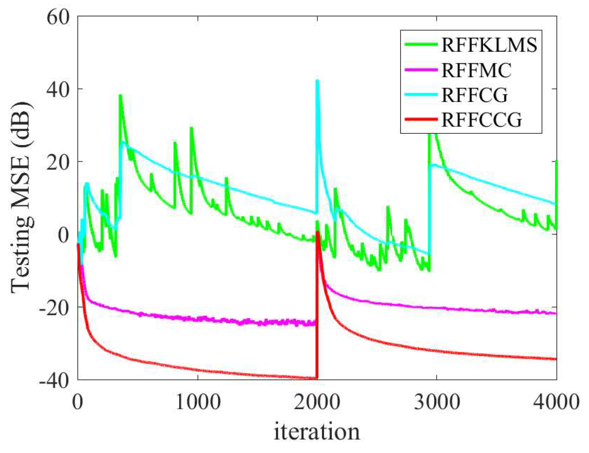
| Algorithm | Size | MSE | Consumed Time |
|---|---|---|---|
| RFFKLMS [13] | 50 | N/A | 2.2773 |
| QKRLS [32] | 160 | N/A | 7.1883 |
| RFFMC [14] | 50 | −23.6263 | 2.3359 |
| KRMC-NC [31] | 500 | −34.3570 | 2.9277 |
| RFFCG [15] | 50 | N/A | 2.3768 |
| RFFCCG | 50 | −38.9975 | 2.3390 |
© 2019 by the authors. Licensee MDPI, Basel, Switzerland. This article is an open access article distributed under the terms and conditions of the Creative Commons Attribution (CC BY) license (http://creativecommons.org/licenses/by/4.0/).
Share and Cite
Huang, X.; Wang, S.; Xiong, K. The Cauchy Conjugate Gradient Algorithm with Random Fourier Features. Symmetry 2019, 11, 1323. https://doi.org/10.3390/sym11101323
Huang X, Wang S, Xiong K. The Cauchy Conjugate Gradient Algorithm with Random Fourier Features. Symmetry. 2019; 11(10):1323. https://doi.org/10.3390/sym11101323
Chicago/Turabian StyleHuang, Xuewei, Shiyuan Wang, and Kui Xiong. 2019. "The Cauchy Conjugate Gradient Algorithm with Random Fourier Features" Symmetry 11, no. 10: 1323. https://doi.org/10.3390/sym11101323
APA StyleHuang, X., Wang, S., & Xiong, K. (2019). The Cauchy Conjugate Gradient Algorithm with Random Fourier Features. Symmetry, 11(10), 1323. https://doi.org/10.3390/sym11101323