1. Introduction, Definitions and Preliminaries
The subject of
q-calculus leads to a new method for computations and classifications of
q-series and
q-polynomials. In fact, the subject of
q-calculus was initiated in the 1920s. However, it has gained considerable popularity and importance during the last three decades or so. In the past decade,
q-calculus was developed into an interdisciplinary subject and it served as a bridge between mathematics and physics. The field has been expanded explosively due mainly to its applications in diverse areas of physics such as cosmic strings and black holes [
1], conformal quantum mechanics [
2], nuclear and high energy physics [
3], fluid mechanics, combinatorics, having connection with commutativity relations, number theory, and Lie algebra. The definitions and notations of the
q-calculus reviewed here are taken from [
4] (see also [
5,
6]).
The
q-analogue of the Pochhammer symbol
, which is also called the
q-shifted factorial, defined by
The
q-analogues of a complex number
and of the factorial function are defined as follows:
and
where
is the set of positive integers.
The
q-binomial coefficients
are defined by
The
q-analogue of the classical derivative
or
of a function
f at a point
is defined by
We also note that
The two familiar
q-analogues of the exponential function
are given by
and
The above-defined
q-exponential functions
and
satisfy the following properties:
The class of Appell polynomials was introduced and characterized completely by Appell [
7] in 1880. Further, Throne [
8], Sheffer [
9] and Varma [
10] studied this class of polynomials from different points of view. For some subsequent and recent developments associated with the Appell polynomials, one may refer to the works [
11,
12,
13,
14].
In the year 1954, Sharma and Chak [
15] introduced a
q-analogue of the Appell polynomials and called this sequence of polynomials as
q-Harmonics. Later, in the year 1967, Al-Salam [
16] introduced the class of the
q-Appell polynomials
and studied some of their properties. Some characterizations of the
q-Appell polynomials were presented by Srivastava [
17] in the year 1982. These polynomials arise in numerous problems of applied mathematics, theoretical physics, approximation theory and many other branches of the mathematical sciences [
7,
18,
19,
20]. The polynomials
(of degree
m) are called
q-Appell polynomials, provided that they satisfy the following
q-differential equation:
Recently, Keleshteri and Mahmudov [
21] introduced the 2D
q-Appell polynomials (2DqAP)
which are defined by means of the following generating function:
where
We write
where
denotes the 2D
q-Appell numbers.
For
, the 2DqAP
reduce to the
q-Appell polynomials
(see, for example, [
16,
17,
22]), that is,
where
are defined by
and
given by
denotes the
q-Appell numbers.
The explicit form of the 2DqAP
in terms qAP
is given as follows (see [
21]):
The function may be called the determining function for the set . Based on suitable selections for the function , the following different members belonging to the family of the 2D q-Appell polynomials can be obtained:
- I.
If
, the 2DqAP
reduce to the 2D
q-Bernoulli polynomials (2DqBP)
(see [
23,
24]), that is,
where
are defined by
and
given by
denotes the 2D
q-Bernoulli numbers.
- II.
If
, the 2DqAP
reduce to the 2D
q-Euler polynomials (2DqEP)
(see [
23,
24]), that is,
where
are defined by
and
given by
denotes the 2D
q-Euler numbers.
- III.
If
, the 2DqAP
reduce to the 2D
q-Genocchi polynomials (2DqGP)
(see [
23,
24]; see also [
25]), that is,
where
are defined by
and
denotes the 2D
q-Genocchi numbers.
We recall here that, in a recent paper, Khan and Riyasat [
26] introduced the twice-iterated
q-Appell polynomials
which are defined by means of the following generating function:
In this paper, the class of the twice-iterated 2D
q-Appell polynomials is introduced by means of generating functions, recurrence relations, partial
q-difference equations, and series and determinant expressions. Further, several results are obtained for the members corresponding to this polynomial family. In
Section 2, the twice-iterated 2D
q-Appell polynomials are introduced by means of the generating functions and series definition. Also, the recurrence relation and
q-difference equations involving the twice-iterated 2D
q-Appell polynomials are derived. In
Section 3, a determinant expression for the twice-iterated 2D
q-Appell polynomials is established. In
Section 4, the determinant expressions and some other properties of the members belonging to the family of the twice-iterated 2D
q-Appell polynomials are obtained.
Section 5 provides several graphical representations and surface plots associated with several members of families of
q-polynomials which have investigated in this paper. Finally, in
Section 6, we present some concluding remarks and observations.
2. Twice-Iterated 2D q-Appell Polynomials
In order to introduce the twice-iterated 2D
q-Appell polynomials (2I2DqAP), we consider two different sets of the 2D
q-Appell polynomials
and
such that
where
where
The generating function for the 2I2DqAP is asserted by the following result.
Theorem 1. The generating function for the twice-iterated 2D
q-Appell polynomials is given by Proof. By expanding the first
q-exponential function
in the left-hand side of the Equation (
20) and then replacing the powers of
x, that is,
by the polynomials
in the left-hand side and
by
in the right-hand side of the resultant equation, we have
Moreover, by summing up the series in the left-hand side and then using the Equation (
24) in the resulting equation, we get
Finally, denoting the resulting 2I2DqAP in the right-hand side of the above equation by
, that is,
the assertion (
25) of Theorem 1 is proved. □
Remark 1. For , the 2I2DqAP reduce to the twice-iterated q-Appell polynomials (see [26]) such thatIt is also noted that We next give the series definition for the 2I2DqAP by proving the following result.
Theorem 2. The twice-iterated 2D
q-Appell polynomials are given by the following series expression: Proof. In view of the Equations (
21) and (
22), the Equation (
25) can be written as follows:
which, on using the Cauchy product rule, gives
Equating the coefficients of like powers of
t in both sides of the above equation, we arrive at the assertion (
31) of Theorem 2. □
Remark 2. For
, the series expression (
31) becomes
which is a known result [
26] (p. 5, Equation (2.8)).
We now state and prove the following result.
Theorem 3. The following relation between the twice-iterated 2D q-Appell polynomials and the twice-iterated q-Appell polynomials holds true: Proof. Using the Equations (
7) and (
19) in the left-hand side of the generating function (
25), we get
which, on applying the Cauchy product rule in the left-hand side, yields
Finally, equating the coefficients of like powers of
t on both sides of this last equation, we obtain the assertion (
35) of Theorem 3. □
Remark 3. By taking in the result (35), we get Remark 4. The following statements are equivalent:and In order to derive the q-recurrence relations and the q-difference equations for the twice-iterated 2D q-Appell polynomials by using the lowering operators that are, in fact, the q-derivative operator , we first prove the following lemma.
Lemma 1. The twice-iterated 2D
q-Appell polynomials satisfy the following operational relations:and Proof. In view of the Equation (
25), the proof of the above lemma requires a direct use of the identity (
5). We, therefore, skip the details involved. □
We now derive the q-recurrence relations for the 2I2DqAP .
Theorem 4. The twice-iterated 2D
q-Appell polynomials satisfy the following linear homogeneous recurrence relation:where Proof. Consider the following generating function:
By taking the
q-derivative of the Equation (
47) partially with respect to
t, we get
Thus, upon factorizing
occurring in the left-hand side and multiplying both sides of the identity (
48) by
t, we find that
In view of the assumption (
46) and the Equation (
47), the Equation (
49) becomes
which, on using the Cauchy product rule, gives
Finally, upon equating the coefficients of like powers of
t on both sides of the above equation and dividing both sides of the resulting equation by
, we get the assertion (
45) of Theorem 4. □
We now state and prove the following result.
Theorem 5. The following recurrence relation for the twice-iterated 2D
q-Appell polynomials holds true: Proof. We first use the Equation (
47) in both sides of the Equation (
49). Then, after some simplification, by equating the coefficients of like powers of
t on both sides of the resulting equation, we arrive at the assertion (
52) of Theorem 5. □
We next derive the q-difference equations which are satisfied by the twice-iterated 2D q-Appell polynomials.
Theorem 6. The twice-iterated 2D
q-Appell polynomials are the solutions of the following q-difference equations:or Proof. The proof of the assertions (
53) and (
54) of Theorem 6 would follow directly upon using the Equations (
43) and (
44), respectively, in the recurrence relation (
45). □
In the next section (
Section 3 below), the determinant forms for the 2I2DqAP are established.
4. Several Members of the Twice-Iterated 2D -Appell Polynomials
During the last two decades, much research work has been done for different members of the family of the q-Appell polynomials and the 2D q-Appell polynomials. By making suitable selections for the functions and , the members belonging to the family of the twice-iterated 2D q-Appell polynomials can be obtained. The 2D q-Bernoulli polynomials , the 2D q-Euler polynomials and the 2D q-Genocchi polynomials are important members of the 2D q-Appell family. Therefore, in this section, we first introduce the 2D q-Euler based Bernoulli polynomials (2DqEBP) and the 2D q-Genocchi based Bernoulli polynomials (2DqGBP) by means of their respective generating functions and series definitions. We then explore other properties of these members.
4.1. The 2D q-Euler–Bernoulli Polynomials
Since, for
the 2DqAP
reduce to the 2DqEP
and the 2DqBP
, respectively. Therefore, for the same choices of
, that is,
the 2I2DqAP reduce to 2DqEBP
and are defined by means of generating functions as follows:
The 2DqEBP
of degree
m are defined by the following series:
The following relation between the 2DqEBP
and the qEBP
holds true:
which, for
, yields
The 2DqEBP
satisfy the following recurrence relation:
Further, by taking
and
in the Equation (56), we obtain the determinant definition of the 2DqEBP
as given below.
Definition 1. The 2D q-Euler–Bernoulli polynomials of degree m are defined bywhere are the 2D q-Euler polynomials of degree m. 4.2. The 2D q-Genocchi–Bernoulli Polynomials
Since, for
the 2DqAP
reduce to the 2DqGP
and the 2DqBP
, respectively. Therefore, for the same choices of
, that is,
the 2I2DqAP reduce to 2DqGBP
and are defined by means of generating functions as follows:
The 2DqGBP
of degree
m are defined by the following series:
The following relation between the 2DqGBP
and the qGBP
holds true:
which, for
, gives
The 2DqGBP
satisfy the following recurrence relation:
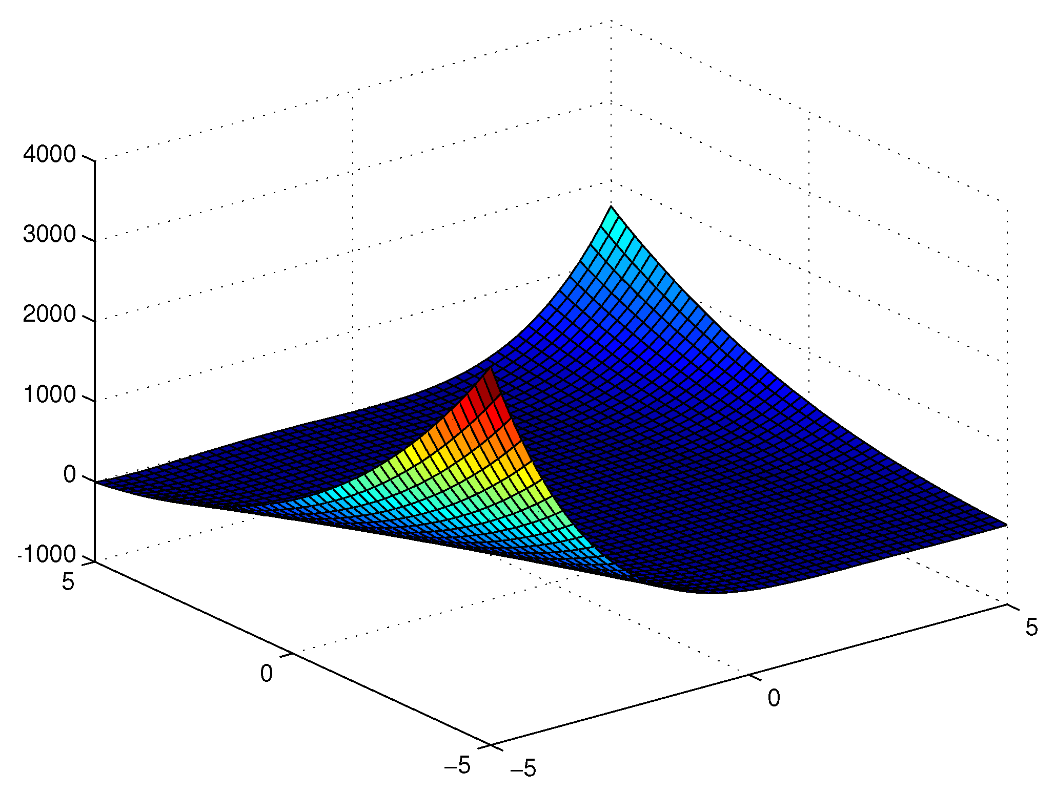
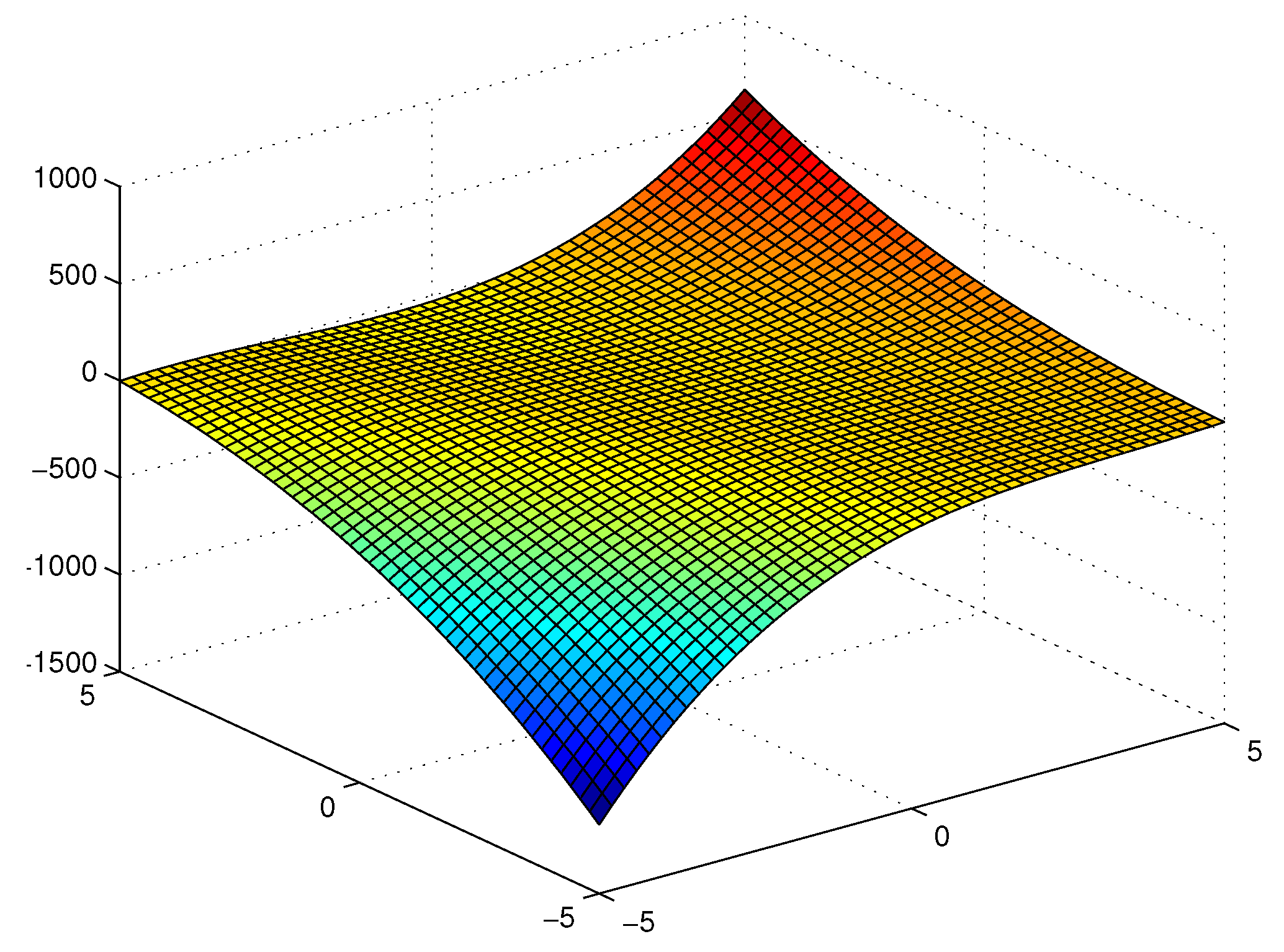
In the next section (
Section 5 below), we give some graphical representations and the surface plots of some of the members of the twice-iterated 2D
q-Appell polynomials.
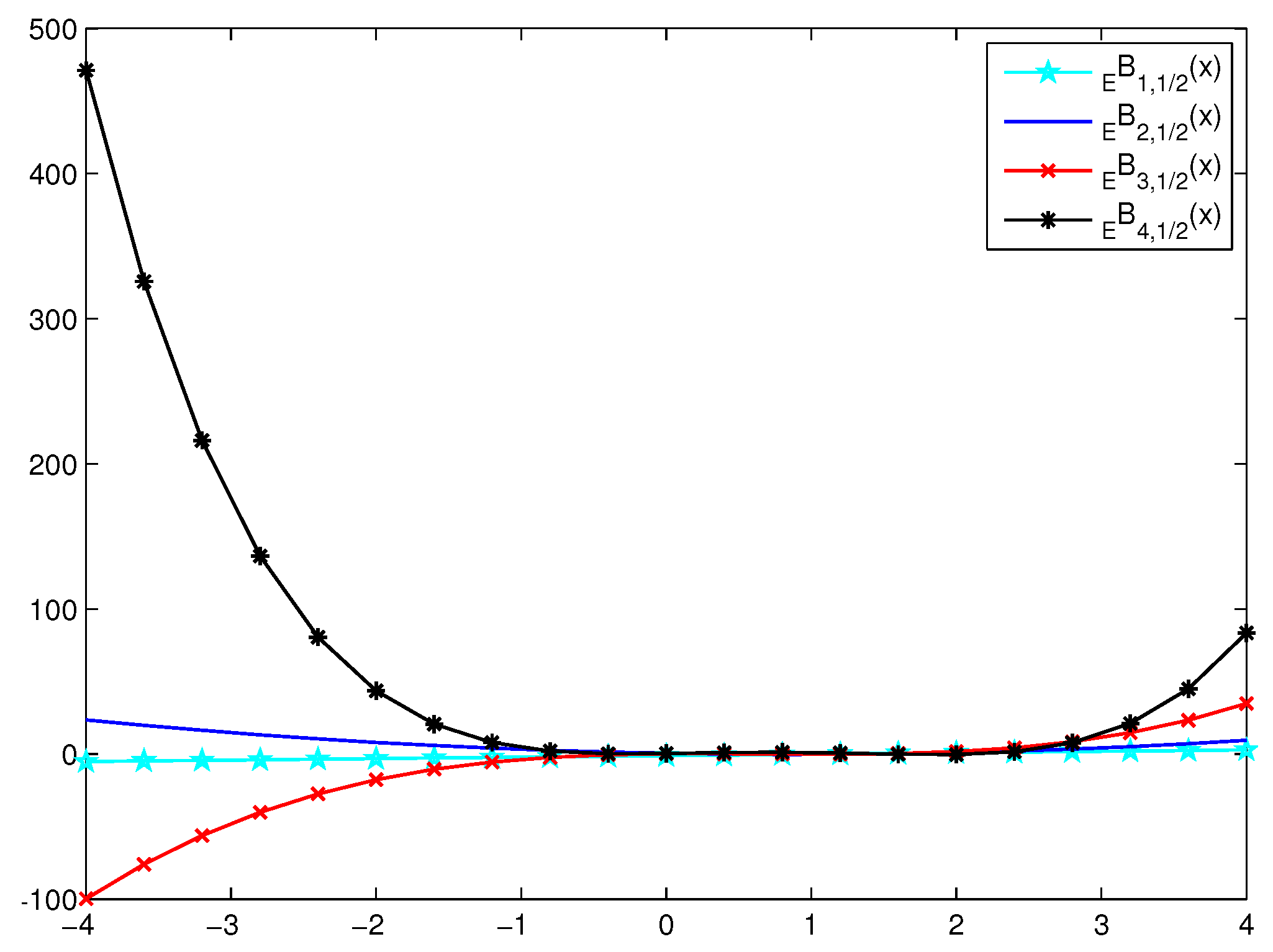
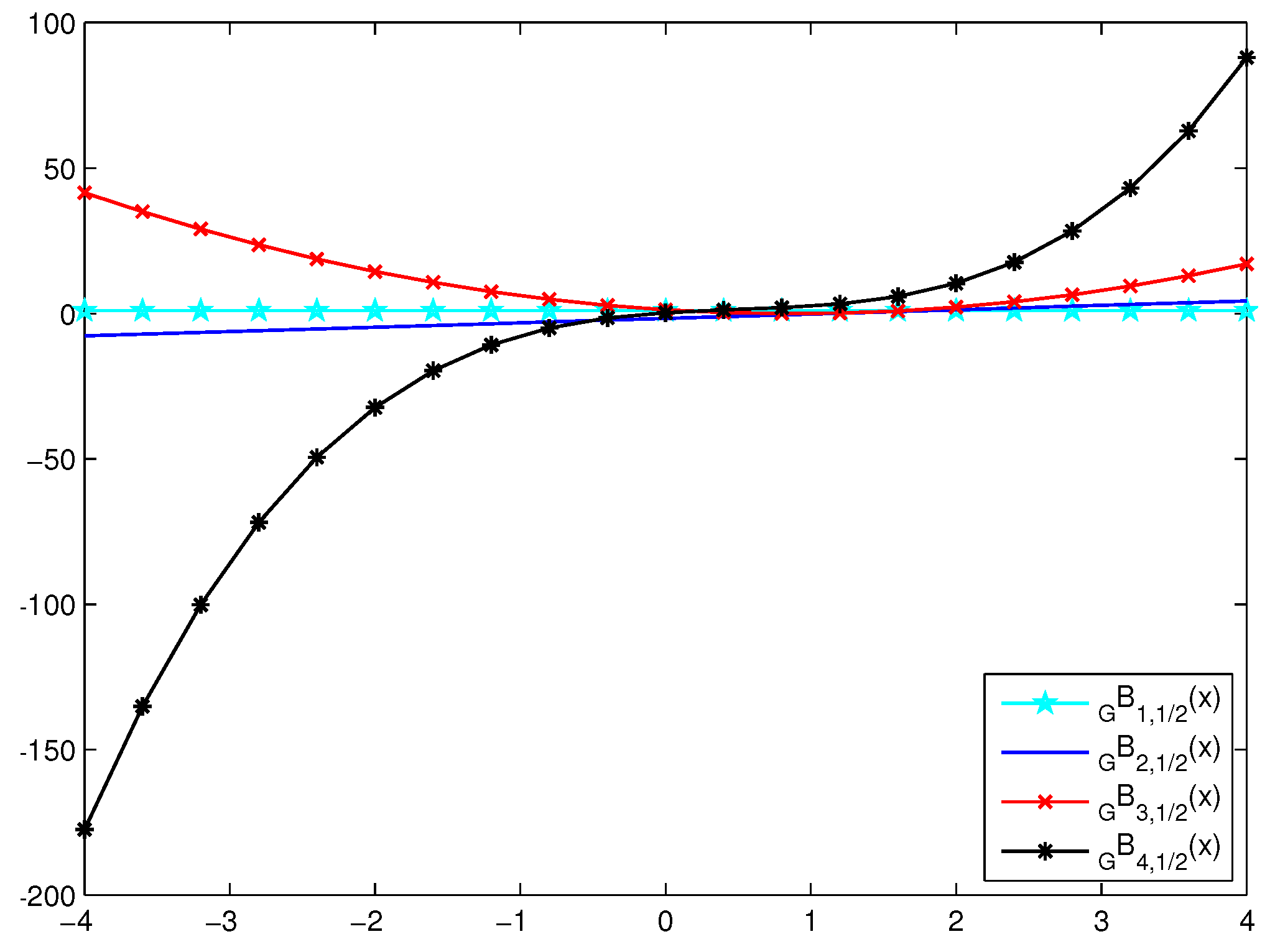
5. Graphical Representations and Surface Plots
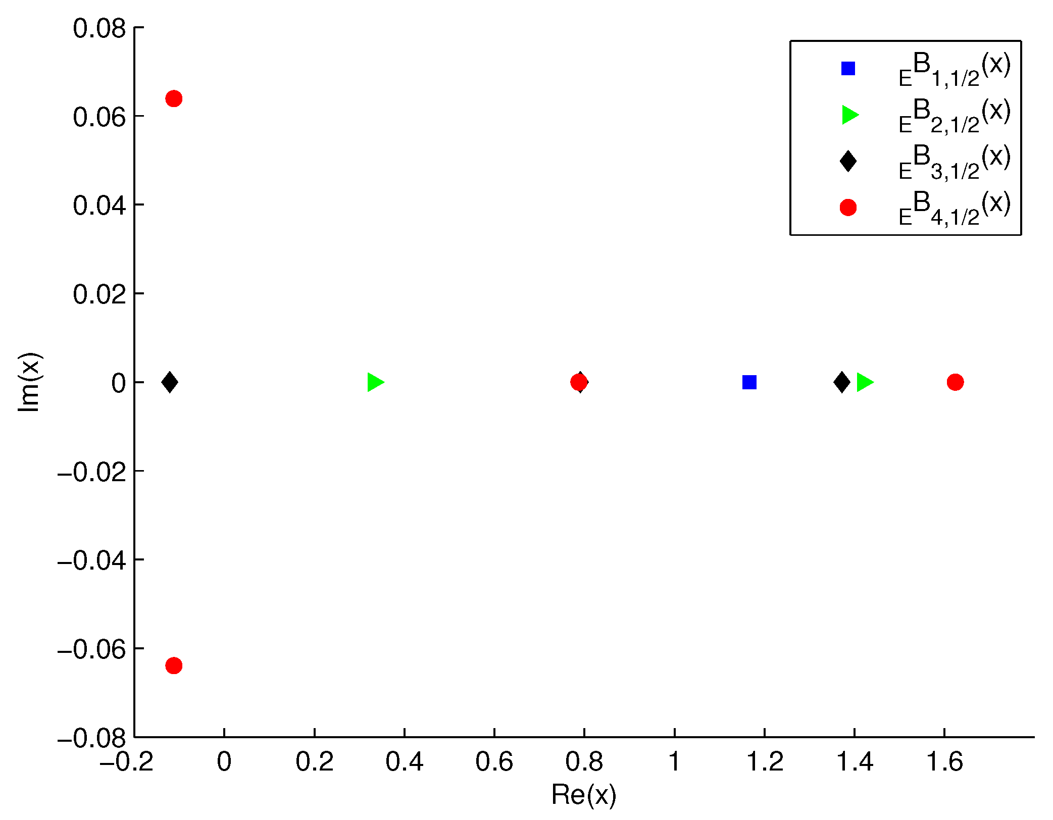
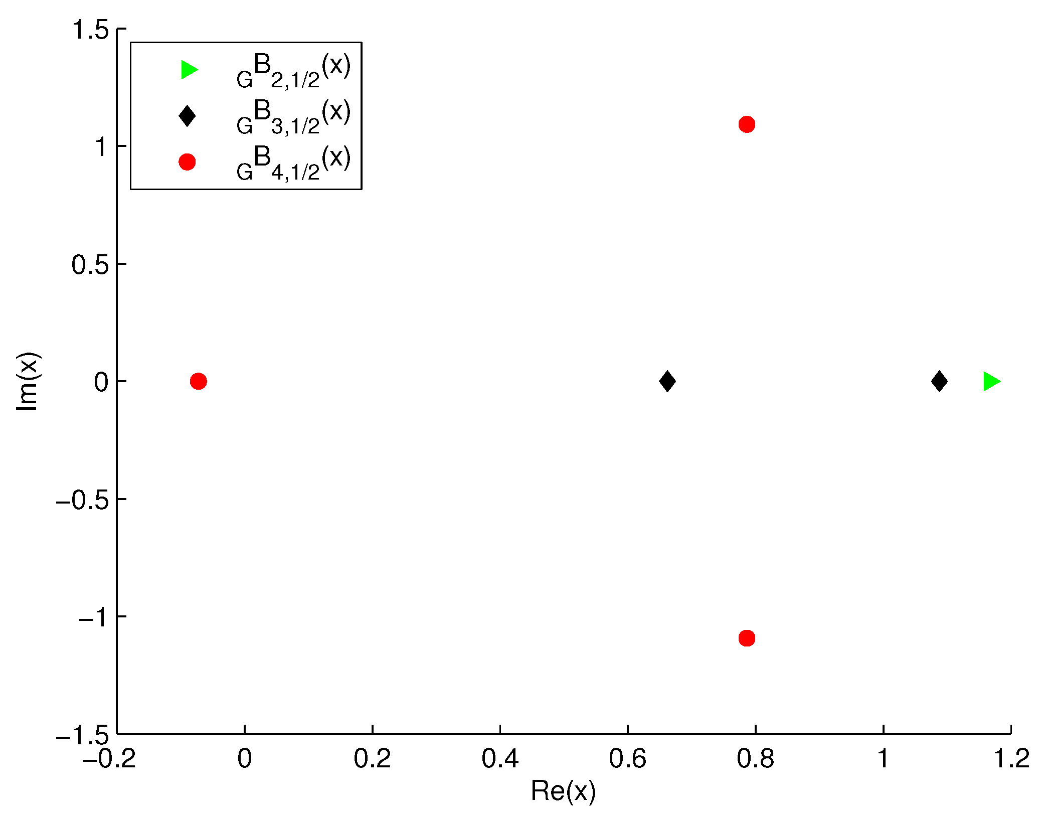
Here, in this section, the graphs of the q-Euler–Bernoulli polynomials (qEBP) , q-Genocchi- Bernoulli polynomials (qGBP) and the surface plots of the 2DqEBP and the 2DqGBP are presented.
To draw the plot of the qEBP
and the qGBP
, we choose
and consider the values of the first four
q-Euler–Bernoulli polynomials and of the first four
q-Genocchi–Bernoulli polynomials, the expressions of these polynomials are given in
Table 1.
Further, by setting
and
in the series definitions (
72) and (
79) of
and
and using the particular values of
and
from
Table 1, we find that
and
Further, with the help of Matlab, we compute the real and complex zeros of
and
for
and
. These zeros are mentioned in
Table 2 and
Table 3.
6. Concluding Remarks and Observations
As long ago as 1910, Jackson [
27] studied the
q-definite integral of an arbitrary function
, which is defined as follows:
and
Applying the double
q-integral to both sides of the Equation (
42), that is,
we have
In view of the Equation (
41), the above Equation (
88) yields
which, on using the Equations (
13) and (
39), becomes
Further, in view of the Equations (
31) and (
34), the Equations (
90) yields
In conclusion, we choose to reiterate the now well-understood fact that the results for the
q-analogues, which we have considered in this article for
, can easily be translated into the corresponding results for the so-called
-analogues (with
) by applying some obviously trivial parametric and argument variations, the additional parameter
p being redundant. In fact, the so-called
-number
is given (for
) by (see also [
28])
where, for the classical
q-number
, we have
Consequently, any claimed extensions of most (including the present) investigations involving the classical q-calculus to the corresponding obviously straightforward investigations involving the -calculus are truly inconsequential.
Further investigations along the lines presented in this paper, which are associated with the various recent generalizations and extensions of the Apostol type Bernoulli, Euler and Genocchi polynomials introduced by, for example, Srivastava et al. (see [
29,
30]) may be worthy of consideration by the targeted readers.


