Lossless Image Compression Techniques: A State-of-the-Art Survey


Abstract
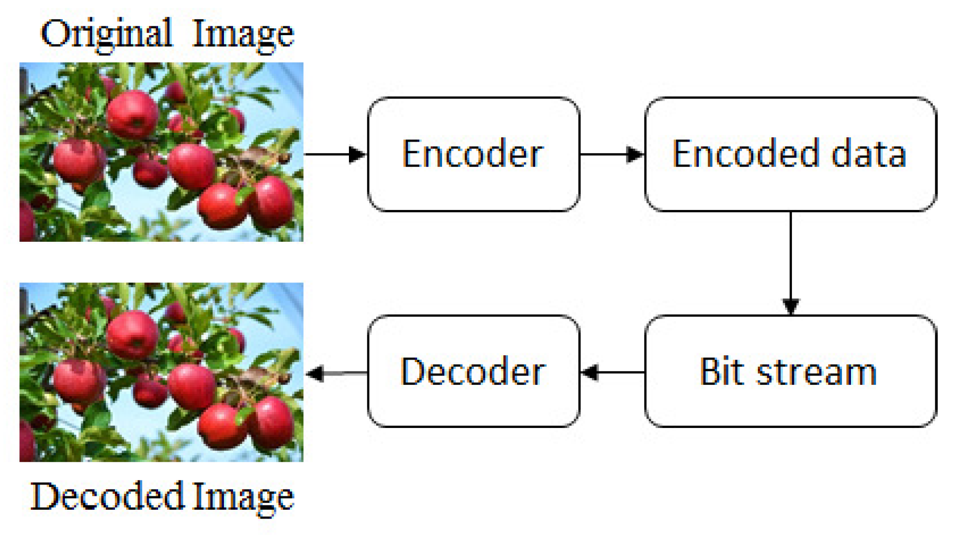
:1. Introduction
2. The State-of-the-Art Techniques
2.1. Run-Length Coding
2.1.1. Run-Length Encoding Procedure
- Calculate the difference (B = [1 −1 0 0 1 0 0 0 0 0 0 0 0 −2 −1 0 0 0 3 0 0 0 0 0 0 0 0 −2 0 0 2 0 −4 0 0 −1 0 0 3 0 0 0 0 0 0 0 0 −4 0 1]) using .
- Assign 1 to each non-zero data of B and we get B = [1 1 0 0 1 0 0 0 0 0 0 0 0 1 1 0 0 0 1 0 0 0 0 0 0 0 0 1 0 0 1 0 1 0 0 1 0 0 1 0 0 0 0 0 0 0 0 1 0 1].
- Save the positions of all ones into an array (position = [1 2 5 14 15 19 28 31 33 36 39 48 50]) and the corresponding data into (items = [6 7 6 7 5 4 7 5 7 3 2 5 1]) from A. The array position and items are stored or sent as the encoded list of the original 50 elements.
2.1.2. Run-Length Decoding Procedure
- Read each element from the array items and write the element repeatedly until its corresponding number in the position array is found.
2.1.3. Analysis of Run-Length Coding Procedure
2.2. Shannon–Fano Coding
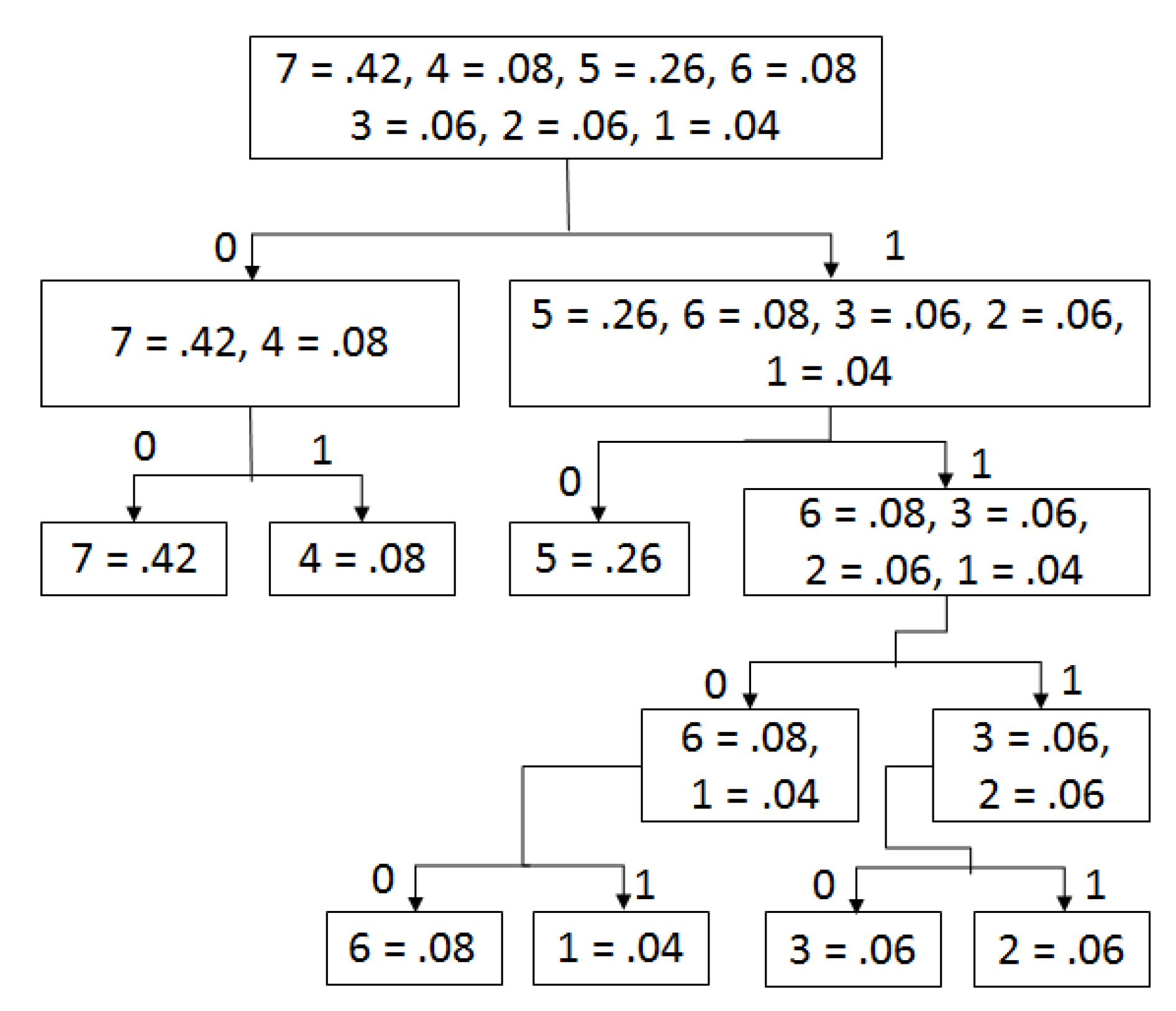
2.2.1. Shannon–Fano Encoding Style
- Find the distinct symbols (N) and their corresponding probabilities.
- Sort the probabilities in descending order.
- Divide them into two groups so that the entire sum of each group is as equal as possible, and make a tree.
- Assign 0 and 1 to the left and right group, respectively.
- Repeat steps 3 and 4 until each element becomes a leaf node on a tree.
2.2.2. Shannon–Fano Decoding Style
- Read each bit from an encoded bitstream and scan the tree until a leaf node is found. At the point when a leaf hub is discovered, read the symbol of the node as decoded value, and the process will proceed until scanning of the encoded bitstream is finished.
2.2.3. Analysis of Shannon–Fano Coding
2.3. Huffman Coding
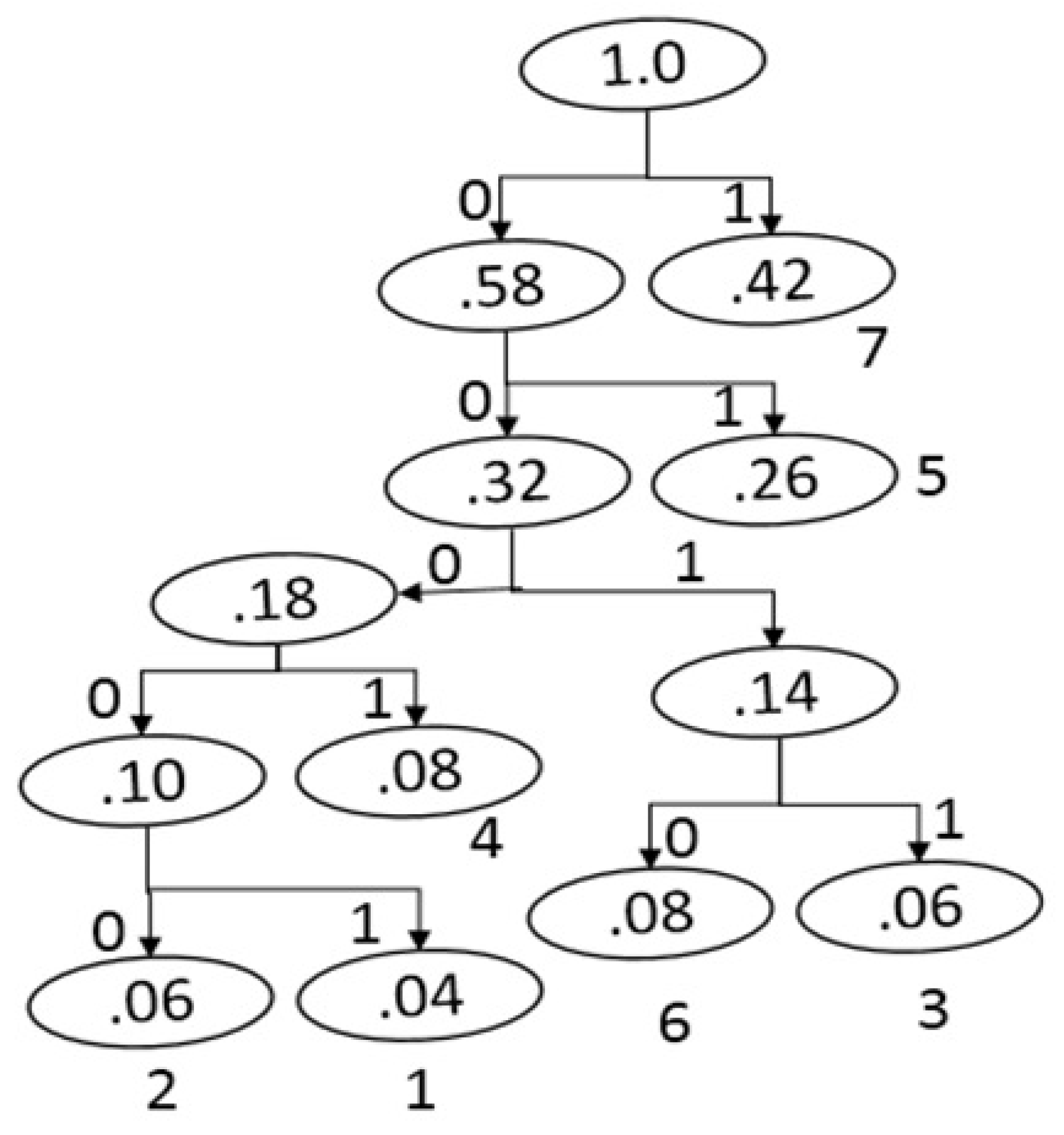
2.3.1. Huffman Encoding Style
- List the probabilities of a gray-scale image in descending order.
- Form a new node of a tree with the sum of the two lowest probabilities on the list and rearrange them in the same order for the proceeding process. This process will continue until the end.
- Assign 0 and 1 to each left and right branch of the tree, respectively.
2.3.2. Huffman Decoding Style
- Recreates the equivalent Huffman tree built in the encoding step using the probabilities.
- Each bit is scanned from the encoded bitstream and traverses the tree node by node until a leaf node is reached. At the point when a leaf node is discovered, the symbol is predicted from the node. This process will proceed until finished.
2.3.3. Analysis of Huffman Coding
2.4. Lempel–Ziv–Welch (LZW) Coding
2.4.1. LZW Encoding Procedure
- Assign 0–255 in a table and set the first data from the input file to FD,
- Repeat steps 3 to 4 until reading is finished,
- ND = Read the next data,
- IF FD + ND is in the table,
- FD = FD + ND,
ELSE- Store the code for FD as encoded data and insert FD + ND to the table. In addition, set FD = ND.
2.4.2. LZW Decoding Procedure
- Assign 0–255 in a table and scan the first encoded value and assign it to FEV. Later, send the translation of FEV to the output.
- Repeat steps 3 to 4 until the reading of the encoded file ends.
- NC = read next code from encoded file.
- IF (NC is not found in the table).
- Assign the translation of FEV to DS and perform DS = DS + NC
ELSE- Assign the translation of NC to DS, the first code of DS to NC, NC to FEV and add FEV+NC into the table. Furthermore, send DS to the output.
2.4.3. Analysis of LZW Coding
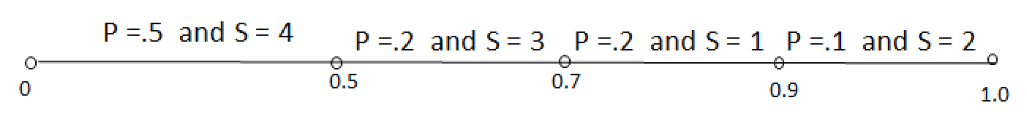
2.5. Arithmetic Coding
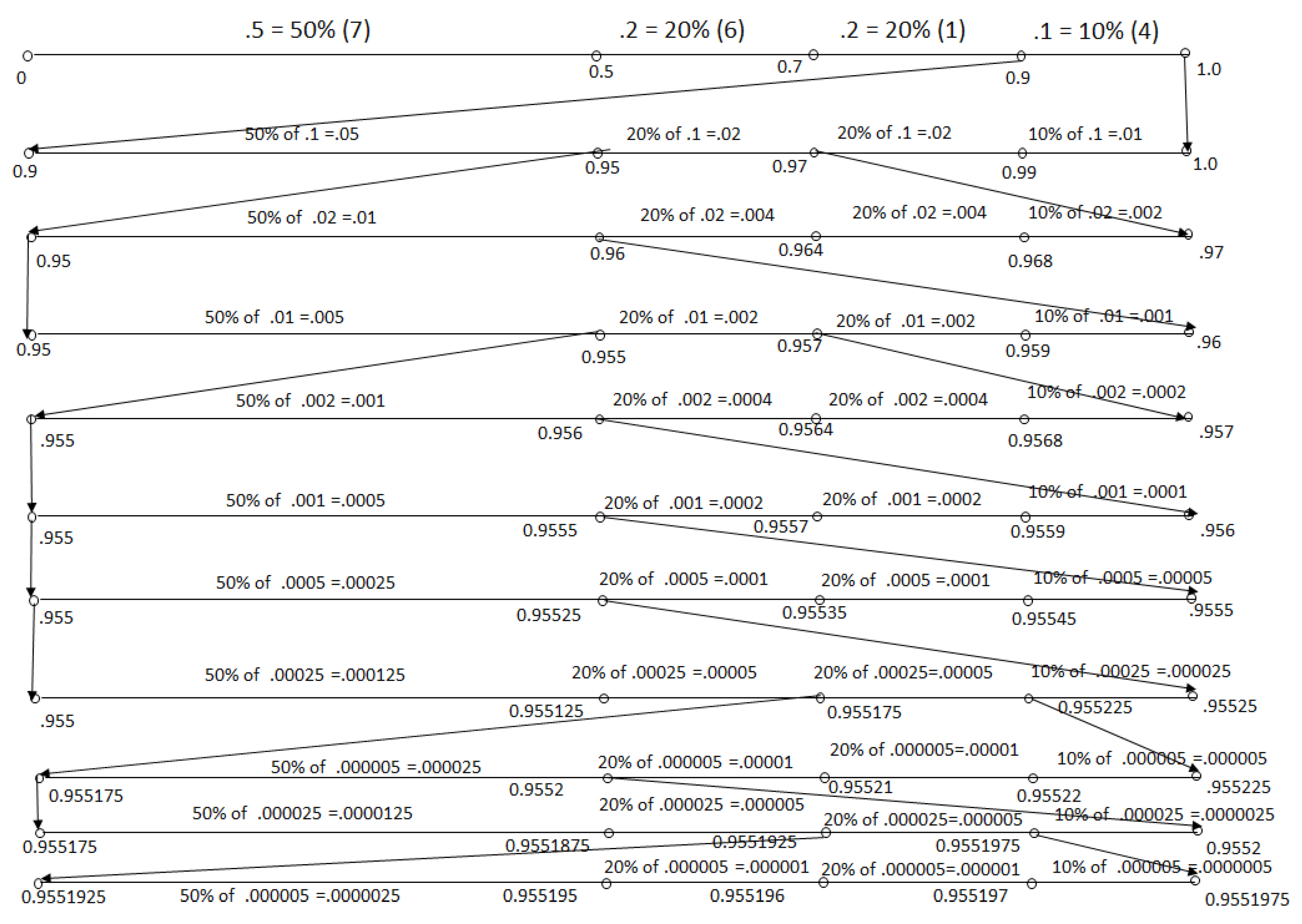
2.5.1. Arithmetic Encoding Procedure
- limit = UL − LL,
- UL = LL + limit * CF[N − 1],
- LL = LL + limit * CF[N].
2.5.2. Arithmetic Decoding Procedure
- if(CF[N] < = (tag − LL)/(UL − LL) < CF[N − 1]),
- (a)
- limit = UL − LL,
- (b)
- UL = LL + limit*CF[N − 1],
- (c)
- LL = LL + limit*CF[N],
- (d)
- return N.
- tag = 0.955195. Since 0.9 < = tag < = 1.0, Thus, decoded value is 2 because the symbol 2 is in range.
- NT1 = (tag − LL)/r = 0.55195 and it is in between 0.5 and 0.7, so the decoded value is 3.
- NT2 = (NT1 − LL)/r = 0.25975 and it is in between 0 and 0.5, so the decoded value is 4.
- NT3 = (NT2 − LL)/r = 0.5195 and it is in between 0.5 and 0.7, so the decoded value is 3.
- NT4 = (NT3 − LL)/r = 0.0975 and it is in between 0 and 0.5, so the decoded value is 4.
- NT5 = (NT4 − LL)/r = 0.195 and it is in between 0 and 0.5, so the decoded value is 4.
- NT6 = (NT5 − LL)/r = 0.39 and it is in between 0 and 0.5, so the decoded value is 4.
- NT7 = (NT6 − LL)/r = 0.78 and it is in between 0.7 and 0.9, so the decoded value is 1.
- NT8 = (NT7 − LL)/r = 0.4 and it is in between 0 and 0.5, so the decoded value is 4.
- NT9 = (NT8 − LL)/r = 0.8 and it is in between 0.7 and 0.9, so the decoded value is 1.
2.5.3. Analysis of Arithmetic Coding Procedure
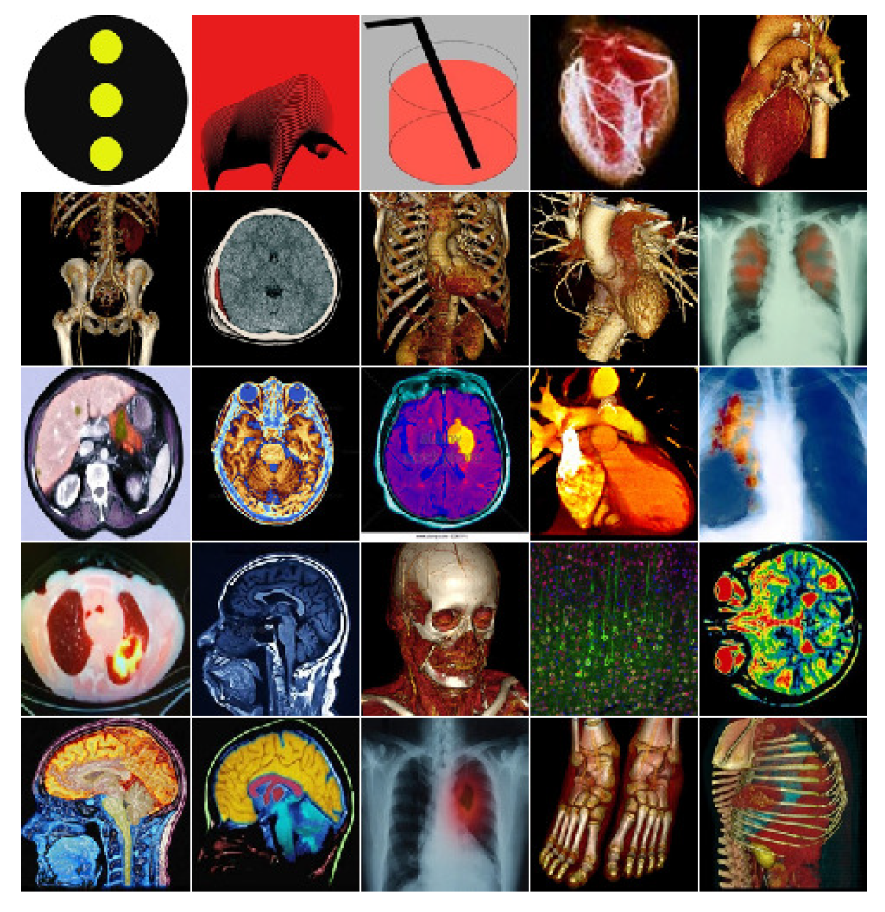
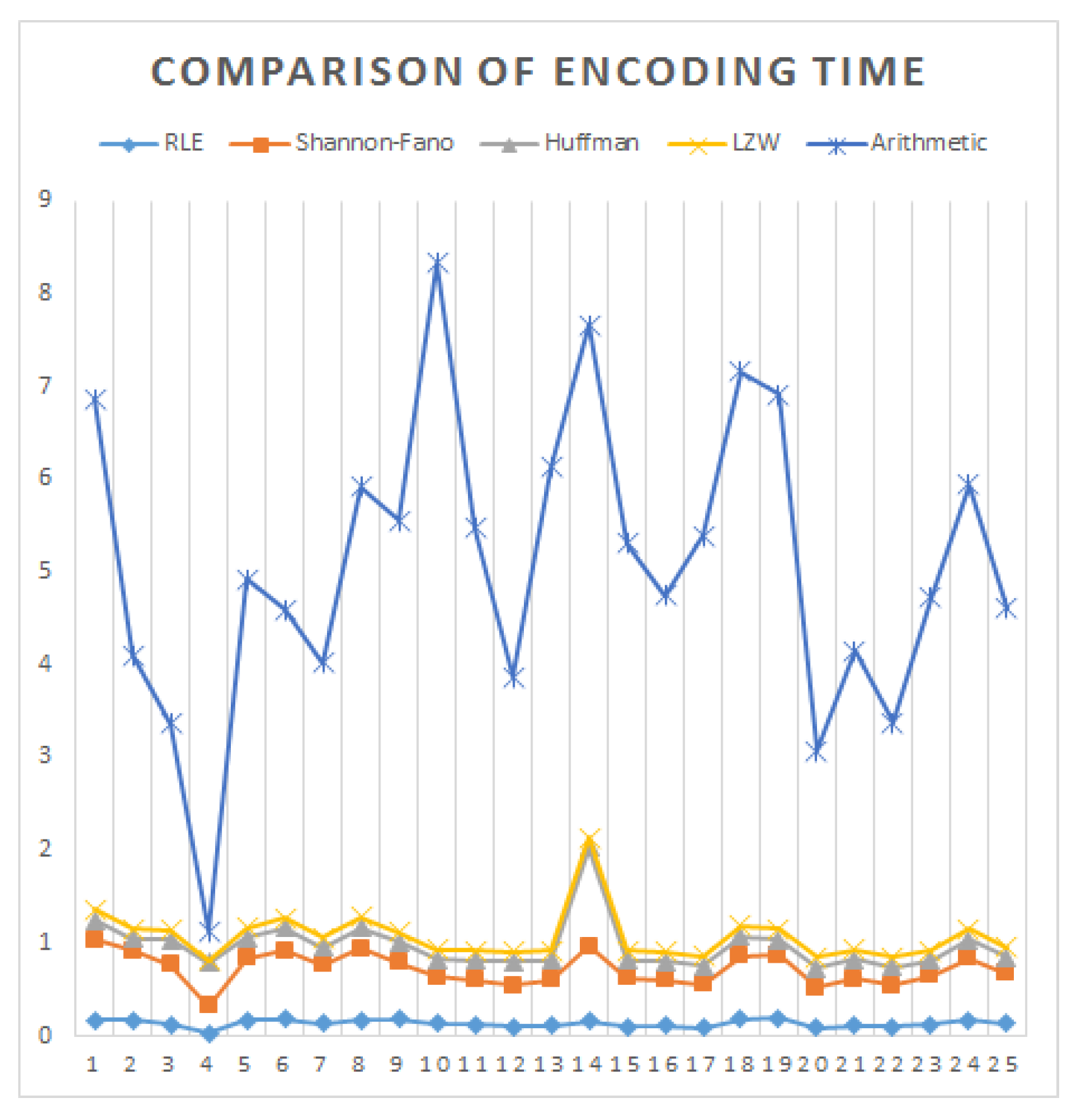
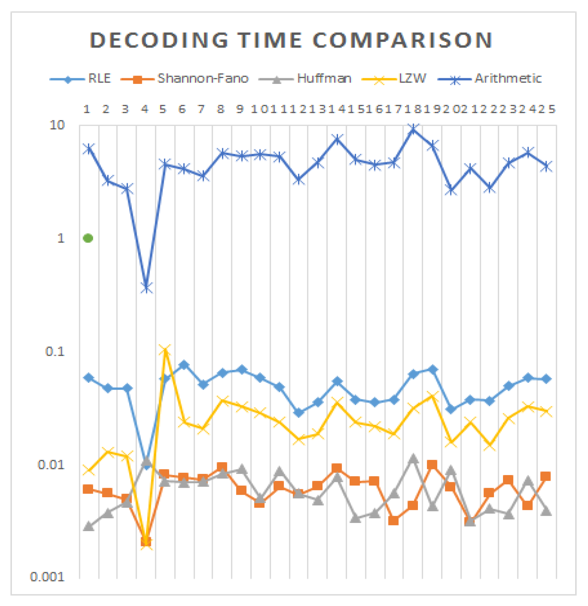
3. Experimental Results and Analysis
4. Conclusions
Author Contributions
Funding
Conflicts of Interest
References
- Bovik, A.C. Handbook of Image and Video Processing; Academic Press: Cambridge, MA, USA, 2010. [Google Scholar]
- Sayood, K. Introduction to Data Compression; Morgan Kaufmann: Burlington, MA, USA, 2017. [Google Scholar]
- Salomon, D.; Motta, G. Handbook of Data Compression; Springer Science & Business Media: Berlin, Germnay, 2010. [Google Scholar]
- Ding, J.; Furgeson, J.C.; Sha, E.H. Application specific image compression for virtual conferencing. In Proceedings of the International Conference on Information Technology: Coding and Computing (Cat. No.PR00540), Las Vegas, NV, USA, 27–29 March 2000; pp. 48–53. [Google Scholar] [CrossRef]
- Bhavani, S.; Thanushkodi, K. A survey on coding algorithms in medical image compression. Int. J. Comput. Sci. Eng. 2010, 2, 1429–1434. [Google Scholar]
- Kharate, G.K.; Patil, V.H. Color Image Compression Based on Wavelet Packet Best Tree. arXiv 2010, arXiv:1004.3276. [Google Scholar]
- Haque, M.R.; Ahmed, F. Image Data Compression with JPEG and JPEG2000. Available online: http://eeweb.poly.edu/~yao/EE3414_S03/Projects/Loginova_Zhan_ImageCompressing_Rep.pdf (accessed on 1 October 2019).
- Clarke, R.J. Digital Compression of still Images And Video; Academic Press, Inc.: Orlando, FL, USA, 1995. [Google Scholar]
- Joshi, M.A. Digital Image Processing: An Algorithm Approach; PHI Learning Pvt. Ltd.: New Delhi, India, 2006. [Google Scholar]
- Golomb, S. Run-length encodings (Corresp). IEEE Trans. Inform. Theory 1966, 12, 399–401. [Google Scholar] [CrossRef]
- Nelson, M.; Gailly, J.L. The Data Compression Book; M & t Books: New York, NY, USA, 1996; Volume 199. [Google Scholar]
- Sharma, M. Compression using Huffman coding. IJCSNS Int. J. Comput. Sci. Netw. Secur. 2010, 10, 133–141. [Google Scholar]
- Burger, W.; Burge, M.J. Digital Image Processing: An Algorithmic Introduction Using Java; Springer: Berlin, Germany, 2016. [Google Scholar]
- Kim, S.D.; Lee, J.H.; Kim, J.K. A new chain-coding algorithm for binary images using run-length codes. Comput. Vis. Graphics Image Process. 1988, 41, 114–128. [Google Scholar] [CrossRef]
- Žalik, B.; Mongus, D.; Lukač, N. A universal chain code compression method. J. Vis. Commun. Image Represent. 2015, 29, 8–15. [Google Scholar] [CrossRef]
- Benndorf, S.; Siemens, A.G. Method for the Compression of Data Using a Run-Length Coding. U.S. Patent 8,374,445, 12 February 2013. [Google Scholar]
- Shanmugasundaram, S.; Lourdusamy, R. A comparative study of text compression algorithms. Int. J. Wisdom Based Comput. 2011, 1, 68–76. [Google Scholar]
- Kodituwakku, S.R.; Amarasinghe, U.S. Comparison of lossless data compression algorithms for text data. Indian J. Comput. Sci. Eng. 2010, 1, 416–425. [Google Scholar]
- Rahman, M.A.; Islam, S.M.S.; Shin, J.; Islam, M.R. Histogram Alternation Based Digital Image Compression using Base-2 Coding. In Proceedings of the 2018 Digital Image Computing: Techniques and Applications (DICTA), Canberra, Australia, 10–13 December 2018; pp. 1–8. [Google Scholar] [CrossRef]
- Drozdek, A. Elements of Data Compression; Brooks/Cole Publishing Co.: Pacific Grove, CA, USA, 2001. [Google Scholar]
- Howard, P.G.; Vitter, J.S. Parallel lossless image compression using Huffman and arithmetic coding. Data Compr. Conf. 1992. [Google Scholar] [CrossRef]
- Pujar, J.H.; Kadlaskar, L.M. A new lossless method of image compression and decompression using Huffman coding techniques. J. Theor. Appl. Inform. Technol. 2010, 15, 15–21. [Google Scholar]
- Mathur, M.K.; Loonker, S.; Saxena, D. Lossless Huffman coding technique for image compression and reconstruction using binary trees. Int. J. Comput. Technol. Appl. 2012, 1, 76–79. [Google Scholar]
- Vijayvargiya, G.; Silakari, S.; Pandey, R. A Survey: Various Techniques of Image Compression. arXiv 2013, arXiv:1311.6877. [Google Scholar]
- Rahman, M.A.; Shin, J.; Saha, A.K.; Rashedul Islam, M. A Novel Lossless Coding Technique for Image Compression. In Proceedings of the 2018 Joint 7th International Conference on Informatics, Electronics & Vision (ICIEV) and 2018 2nd International Conference on Imaging, Vision & Pattern Recognition (ic4PR), Kitakyushu, Japan, 25–29 June 2018; pp. 82–86. [Google Scholar] [CrossRef]
- Rufai, A.M.; Anbarjafari, G.; Demirel, H. Lossy medical image compression using Huffman coding and singular value decomposition. In Proceedings of the 2013 21st Signal Processing and Communications Applications Conference (SIU), Haspolat, Turkey, 24–26 April 2013; pp. 1–4. [Google Scholar] [CrossRef]
- Jasmi, R.P.; Perumal, B.; Rajasekaran, M.P. Comparison of image compression techniques using huffman coding, DWT and fractal algorithm. In Proceedings of the 2015 International Conference on Computer Communication and Informatics (ICCCI), Coimbatore, India, 8–10 January 2015; pp. 1–5. [Google Scholar]
- Xue, T.; Zhang, Y.; Shen, Y.; Zhang, Z.; You, X.; Zhang, C. Adaptive Spatial Modulation Combining BCH Coding and Huffman Coding. In Proceedings of the 2018 IEEE 23rd International Conference on Digital Signal Processing (DSP), Shanghai, China, 19–21 November 2018; pp. 1–5. [Google Scholar] [CrossRef]
- Witten, I.H.; Neal, R.M.; Cleary, J.G. Arithmetic Coding for Data Compression. Commun. ACM 1987, 30, 520–540. [Google Scholar] [CrossRef]
- Masmoudi, A.; Masmoudi, A. A new arithmetic coding model for a block-based lossless image compression based on exploiting inter-block correlation. Signal Image Video Process. 2015, 9, 1021–1027. [Google Scholar] [CrossRef]
- Masmoudi, A.; Puech, W.; Masmoudi, A. An improved lossless image compression based arithmetic coding using mixture of non-parametric distributions. Multimed. Tools Appl. 2015, 74, 10605–10619. [Google Scholar] [CrossRef]
- Weinberger, M.J.; Seroussi, G.; Sapiro, G. The LOCO-I lossless image compression algorithm: Principles and standardization into JPEG-LS. IEEE Trans. Image Process. 2000, 9, 1309–1324. [Google Scholar] [CrossRef]
- Li, X.; Orchard, M.T. Edge directed prediction for lossless compression of natural images. IEEE Trans. Image Proc. 2001, 6, 813–817. [Google Scholar]
- Sasilal, L.; Govindan, V.K. Arithmetic Coding-A Reliable Implementation. Int. J. Comput. Appl. 2013, 73, 7. [Google Scholar] [CrossRef]
- Ding, J.J.; Wang, I.H. Improved frequency table adjusting algorithms for context-based adaptive lossless image coding. In Proceedings of the 2016 IEEE International Conference on Consumer Electronics-Taiwan (ICCE-TW), Nantou, Taiwan, 27–29 May 2016; pp. 1–2. [Google Scholar]
- Rahman, M.A.; Fazle Rabbi, M.M.; Rahman, M.M.; Islam, M.M.; Islam, M.R. Histogram modification based lossy image compression scheme using Huffman coding. In Proceedings of the 2018 4th International Conference on Electrical Engineering and Information & Communication Technology (iCEEiCT), Dhaka, Bangladesh, 13–15 September 2018; pp. 279–284. [Google Scholar] [CrossRef]
- Pennebaker, W.B.; Mitchell, J.L. JPEG: Still Image Data Compression Standard; Springer Science & Business Media: New York, NY, USA, 1992. [Google Scholar]
- Clunie, D.A. Lossless compression of grayscale medical images: effectiveness of traditional and state-of-the-art approaches. In Proceedings of the Medical Imaging 2000: PACS Design and Evaluation: Engineering and Clinical Issues, San Diego, CA, USA, 12–18 February 2000; pp. 74–85. [Google Scholar] [CrossRef]
- Kim, J.; Kyung, C.M. A lossless embedded compression using significant bit truncation for HD video coding. IEEE Trans. Circuits Syst. Video Technol. 2010, 20, 848–860. [Google Scholar]
- Kato, M.; Sony Corp. Motion Video Coding with Adaptive Precision for DC Component Coefficient Quantization and Variable Length Coding. U.S. Patent 5,559,557, 24 September 1996. [Google Scholar]
- Lamorahan, C.; Pinontoan, B.; Nainggolan, N. Data Compression Using Shannon–Fano Algorithm. Jurnal Matematika dan Aplikasi 2013, 2, 10–17. [Google Scholar] [CrossRef]
- Yokoo, H. Improved variations relating the Ziv-Lempel and Welch-type algorithms for sequential data compression. IEEE Trans. Inform. Theory 1992, 38, 73–81. [Google Scholar] [CrossRef]
- Saravanan, C.; Surender, M. Enhancing efficiency of huffman coding using Lempel Ziv coding for image compression. Int. J. Soft Comput. Eng. 2013, 6, 2231–2307. [Google Scholar]
- Pu, I.M. Fundamental Data Compression; Butterworth-Heinemann: Oxford, UK, 2005. [Google Scholar]
- Shannon, C.E. A mathematical theory of communication. ACM SIGMOBILE Mobile Comput. Commun. Rev. 2001, 5, 3–55. [Google Scholar] [CrossRef]
- Huffman, D.A. A method for the construction of minimum-redundancy codes. Proc. IRE 1952, 40, 1098–1101. [Google Scholar] [CrossRef]
- Hussain, A.J.; Al-Fayadh, A.; Radi, N. Image compression techniques: A survey in lossless and lossy algorithms. Neurocomputing 2018, 300, 44–69. [Google Scholar] [CrossRef]
- Zhou, Y.-L.; Fan, X.-P.; Liu, S.-Q.; Xiong, Z.-Y. Improved LZW algorithm of lossless data compression for WSN. In Proceedings of the 2010 3rd International Conference on Computer Science and Information Technology, Chengdu, China, 9–11 July 2010; pp. 523–527. [Google Scholar] [CrossRef]
- Ziv, J.; Lempel, A. A universal algorithm for sequential data compression. IEEE Trans. Inform. Theory 1977, 23, 337–343. [Google Scholar] [CrossRef]
- Rahman, M.A.; Jannatul Ferdous, M.; Hossain, M.M.; Islam, M.R.; Hamada, M. A lossless speech signal compression technique. In Proceedings of the 1st International Conference on Advances in Science, Engineering and Robotics Technology, Dhaka, Bangladesh, 3–5 May 2019. [Google Scholar]
- Langdon, G.G. An introduction to arithmetic coding. IBM J. Res. Dev. 1984, 28, 135–149. [Google Scholar] [CrossRef]
- Osirix-viewer.com. 2019. OsiriX DICOM Viewer | DICOM Image Library. Available online: https://www.osirix-viewer.com/resources/dicom-image-library/ (accessed on 10 April 2019).

| i | CR | BPP | |||||
|---|---|---|---|---|---|---|---|
| 7 | 0.42 | 00 | 2 | 0.84 | −0.526 | 3.226 | 0.31 |
| 4 | 0.08 | 01 | 2 | 0.52 | −0.292 | ||
| 5 | 0.26 | 10 | 2 | 0.16 | −0.505 | ||
| 6 | 0.08 | 1100 | 4 | 0.32 | −0.292 | ||
| 3 | 0.06 | 1110 | 4 | 0.24 | −0.244 | ||
| 2 | 0.06 | 1111 | 4 | 0.24 | −0.244 | ||
| 1 | 0.04 | 1101 | 4 | 0.16 | −0.186 | ||
| ACL = 2.48 | Entropy = 2.289 |
| i | CR | BPP | |||||
|---|---|---|---|---|---|---|---|
| 7 | 0.42 | 1 | 1 | 0.42 | −0.526 | 3.448 | 0.29 |
| 5 | 0.26 | 01 | 2 | 0.52 | −0.505 | ||
| 4 | 0.08 | 0001 | 4 | 0.32 | −0.292 | ||
| 6 | 0.08 | 0010 | 4 | 0.32 | −0.292 | ||
| 3 | 0.06 | 0011 | 4 | 0.24 | −0.244 | ||
| 2 | 0.06 | 00000 | 5 | 0.3 | −0.244 | ||
| 1 | 0.04 | 00001 | 5 | 0.2 | −0.186 | ||
| ACL = 2.32 | Entropy = 2.289 |
| Row Number | Encoded Output | Dictionary | |
|---|---|---|---|
| Index | Entry | ||
| 1 | - | 1 | 1 |
| 2 | - | 2 | 2 |
| 3 | - | 3 | 3 |
| 4 | - | 4 | 4 |
| 5 | - | 5 | 5 |
| 6 | - | 6 | 6 |
| 7 | - | 7 | 7 |
| 8 | 1 | 8 | 16 |
| 9 | 6 | 9 | 67 |
| 10 | 7 | 10 | 76 |
| 11 | 6 | 11 | 66 |
| 12 | 9 | 12 | 677 |
| 13 | 7 | 13 | 77 |
| 14 | 7 | 14 | 74 |
| 15 | 4 | 15 | 47 |
| 16 | 13 | 16 | 777 |
| 17 | 13 | 17 | 775 |
| 18 | 5 | 18 | 57 |
| 19 | 14 | 19 | 744 |
| 20 | 15 | 20 | 474 |
| 21 | 15 | 21 | 477 |
| 22 | 16 | 22 | 7777 |
| 23 | 16 | 23 | 7775 |
| 24 | 18 | 24 | 577 |
| 25 | 7 | 25 | 75 |
| 26 | 5 | 26 | 55 |
| 27 | 24 | 27 | 5773 |
| 28 | 3 | 28 | 33 |
| 29 | 3 | 29 | 32 |
| 30 | 2 | 30 | 23 |
| 31 | 29 | 31 | 322 |
| 32 | 2 | 32 | 25 |
| 33 | 26 | 33 | 555 |
| 34 | 26 | 34 | 556 |
| 35 | 6 | 35 | 65 |
| 36 | 33 | 36 | 5555 |
| 37 | 26 | 37 | 551 |
| 38 | 1 | - | - |
| 39 | 0 | Stop Code | |
| Encoded Data | Encoded Bit’s Stream (6 Bits Each) | ACL | CR |
|---|---|---|---|
| 1 6 7 6 9 7 7 4 13 13 5 14 15 15 16 16 18 7 5 24 3 3 2 29 2 26 26 6 33 26 1 0 | 0000010001100001110001100010 0100011100011100010000110100 1101000101001110001111001111 0100000100000100100001110001 0101100000001100001100001001 1101000010011010011010000110 100001011010000001000000 | 3.84 | 2.083 |
| Initial Dictionary | |
|---|---|
| Index | Entry |
| 1 | 1 |
| 2 | 2 |
| 3 | 3 |
| 4 | 4 |
| 5 | 5 |
| 6 | 6 |
| 7 | 7 |
| Row Number | Code | Output | Full | Conjecture |
|---|---|---|---|---|
| 1 | 1 | 1 | 8: 1? | |
| 2 | 6 | 6 | 8: 16 | 9: 6? |
| 3 | 7 | 7 | 9: 67 | 10: 7? |
| 4 | 6 | 6 | 10: 76 | 11: 6? |
| 5 | 9 | 67 | 11:66 | 12: 67? |
| 6 | 7 | 7 | 12: 677 | 13: 7? |
| 7 | 7 | 7 | 13:77 | 14: 7? |
| 8 | 4 | 4 | 14:74 | 15: 4? |
| 9 | 13 | 77 | 15:47 | 16: 77? |
| 10 | 13 | 77 | 16: 777 | 17: 77? |
| 11 | 5 | 5 | 17:775 | 18:5? |
| 12 | 14 | 74 | 18:57 | 19:74? |
| 13 | 15 | 47 | 19:744 | 20:47? |
| 14 | 15 | 47 | 20:474 | 21:47? |
| 15 | 16 | 777 | 21:477 | 22:777? |
| 16 | 16 | 777 | 22:7777 | 23:777? |
| 17 | 18 | 57 | 23:7775 | 24: 57? |
| 18 | 7 | 7 | 24:577 | 25:7? |
| 19 | 5 | 5 | 25:75 | 26: 5? |
| 20 | 24 | 577 | 26:55 | 27:577? |
| 21 | 3 | 3 | 27:5773 | 28:3? |
| 22 | 3 | 3 | 28:33 | 29:3? |
| 23 | 2 | 2 | 29: 32 | 30: 2? |
| 24 | 29 | 32 | 30:23 | 31: 32? |
| 25 | 2 | 2 | 31:322 | 32:2? |
| 26 | 26 | 55 | 32:25 | 33:55? |
| 27 | 26 | 55 | 33:555 | 34:55? |
| 28 | 6 | 6 | 34:556 | 35:6? |
| 29 | 33 | 555 | 35:65 | 36:555? |
| 30 | 26 | 55 | 37:5555 | 38:55? |
| 31 | 1 | 1 |
| Images | RLE | Shannon–Fano | Huffman | LZW | Arithmetic |
|---|---|---|---|---|---|
| 1 | 0.171 | 0.8667 | 0.2056 | 0.123 | 5.5032 |
| 2 | 0.167 | 0.7524 | 0.1304 | 0.105 | 2.9515 |
| 3 | 0.121 | 0.6455 | 0.2673 | 0.109 | 2.223 |
| 4 | 0.027 | 0.2983 | 0.4699 | 0.022 | 0.3101 |
| 5 | 0.167 | 0.6735 | 0.215 | 0.106 | 3.7628 |
| 6 | 0.187 | 0.7304 | 0.2534 | 0.106 | 3.3215 |
| 7 | 0.141 | 0.6262 | 0.1925 | 0.105 | 2.9568 |
| 8 | 0.165 | 0.7816 | 0.2183 | 0.118 | 4.6419 |
| 9 | 0.186 | 0.6002 | 0.2252 | 0.107 | 4.4352 |
| 10 | 0.137 | 0.5079 | 0.1816 | 0.106 | 7.3937 |
| 11 | 0.126 | 0.4753 | 0.2182 | 0.106 | 4.5515 |
| 12 | 0.096 | 0.449 | 0.2545 | 0.106 | 2.9656 |
| 13 | 0.113 | 0.4942 | 0.2034 | 0.11 | 5.2077 |
| 14 | 0.161 | 0.8058 | 1.0607 | 0.108 | 5.525 |
| 15 | 0.102 | 0.5208 | 0.1932 | 0.106 | 4.3877 |
| 16 | 0.112 | 0.4978 | 0.1979 | 0.106 | 3.8302 |
| 17 | 0.092 | 0.4684 | 0.1939 | 0.106 | 4.5352 |
| 18 | 0.186 | 0.6756 | 0.2139 | 0.118 | 5.9698 |
| 19 | 0.189 | 0.687 | 0.166 | 0.116 | 5.7538 |
| 20 | 0.086 | 0.4395 | 0.2088 | 0.111 | 2.227 |
| 21 | 0.112 | 0.5085 | 0.2059 | 0.106 | 3.217 |
| 22 | 0.103 | 0.4413 | 0.2007 | 0.11 | 2.5256 |
| 23 | 0.122 | 0.5298 | 0.1617 | 0.105 | 3.8022 |
| 24 | 0.172 | 0.6697 | 0.2004 | 0.107 | 4.7927 |
| 25 | 0.132 | 0.5369 | 0.1818 | 0.106 | 3.6537 |
| Average | 0.1349 | 0.5873 | 0.2488 | 0.1054 | 4.0178 |
| Images | RLE | Shannon–Fano | Huffman | LZW | Arithmetic |
|---|---|---|---|---|---|
| 1 | 0.059 | 0.0061 | 0.0029 | 0.009 | 6.2899 |
| 2 | 0.048 | 0.0056 | 0.0038 | 0.013 | 3.273 |
| 3 | 0.048 | 0.005 | 0.0047 | 0.012 | 2.774 |
| 4 | 0.01 | 0.0021 | 0.011 | 0.002 | 0.3718 |
| 5 | 0.058 | 0.0082 | 0.0072 | 0.106 | 4.5912 |
| 6 | 0.078 | 0.0077 | 0.007 | 0.024 | 4.1704 |
| 7 | 0.052 | 0.0075 | 0.0071 | 0.021 | 3.6072 |
| 8 | 0.066 | 0.0096 | 0.0084 | 0.037 | 5.7222 |
| 9 | 0.07 | 0.0059 | 0.0093 | 0.033 | 5.4118 |
| 10 | 0.059 | 0.0046 | 0.0051 | 0.029 | 5.6243 |
| 11 | 0.049 | 0.0065 | 0.0089 | 0.024 | 5.347 |
| 12 | 0.029 | 0.0055 | 0.0056 | 0.017 | 3.3815 |
| 13 | 0.036 | 0.0065 | 0.0049 | 0.019 | 4.7372 |
| 14 | 0.055 | 0.0094 | 0.0078 | 0.036 | 7.6486 |
| 15 | 0.038 | 0.0071 | 0.0034 | 0.024 | 5.0222 |
| 16 | 0.036 | 0.0072 | 0.0038 | 0.022 | 4.5165 |
| 17 | 0.038 | 0.0032 | 0.0056 | 0.019 | 4.7644 |
| 18 | 0.064 | 0.0044 | 0.0116 | 0.032 | 9.3636 |
| 19 | 0.071 | 0.0101 | 0.0043 | 0.041 | 6.7193 |
| 20 | 0.031 | 0.0064 | 0.0092 | 0.016 | 2.7133 |
| 21 | 0.038 | 0.0031 | 0.0032 | 0.024 | 4.2221 |
| 22 | 0.037 | 0.0056 | 0.0041 | 0.015 | 2.8519 |
| 23 | 0.05 | 0.0074 | 0.0037 | 0.026 | 4.696 |
| 24 | 0.059 | 0.0043 | 0.0074 | 0.033 | 5.7915 |
| 25 | 0.058 | 0.0079 | 0.004 | 0.03 | 4.4087 |
| Average | 0.0495 | 0.0063 | 0.0062 | 0.0266 | 4.7208 |
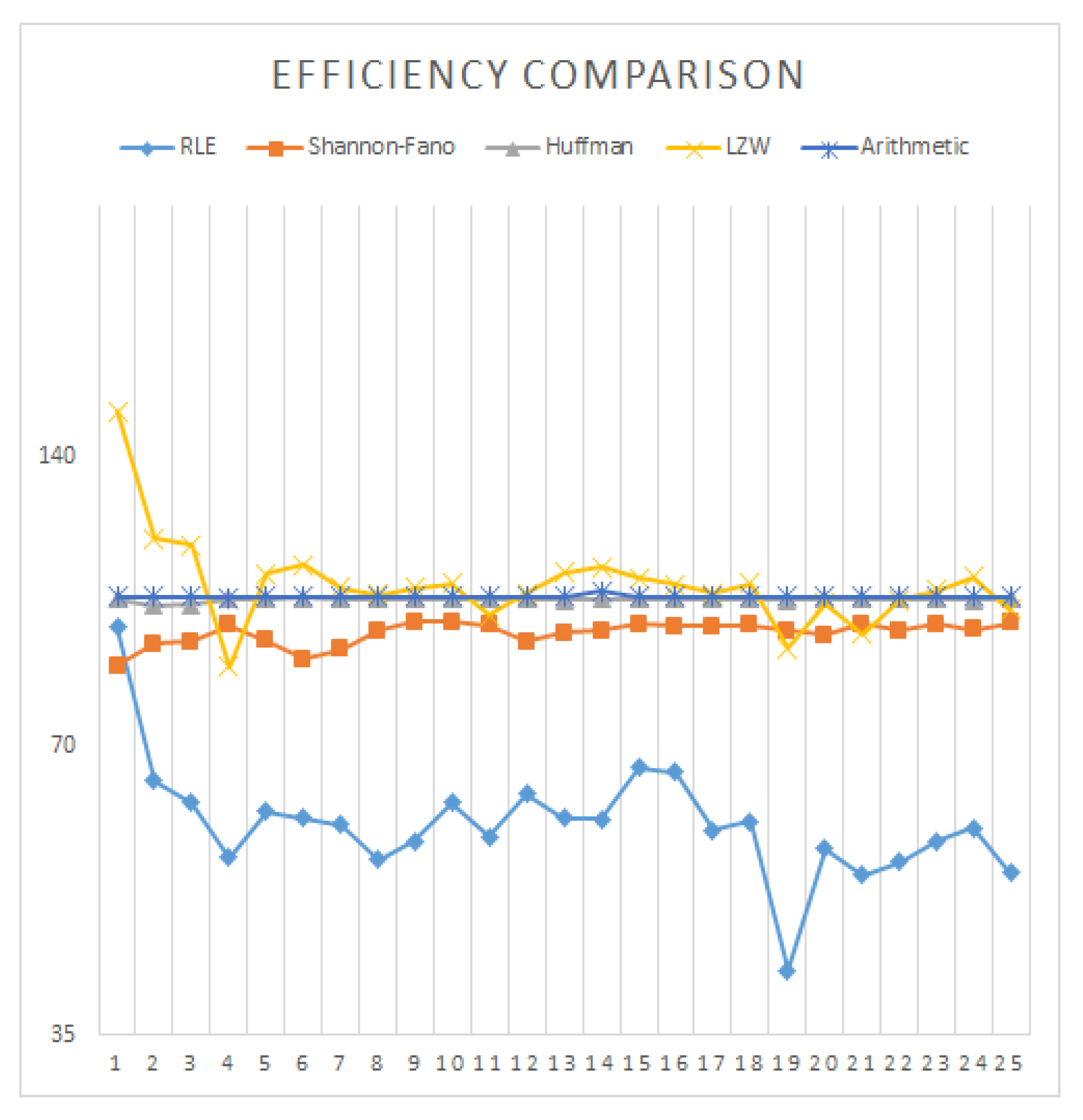
| Images | RLE | Shannon–Fano | Huffman | LZW | Arithmetic |
|---|---|---|---|---|---|
| 1 | 2.6114 | 2.861 | 2.4394 | 1.554 | 2.4265 |
| 2 | 5.0743 | 3.649 | 3.3302 | 2.8331 | 3.264 |
| 3 | 5.9338 | 4.035 | 3.6893 | 3.2044 | 3.6267 |
| 4 | 11.6135 | 6.652 | 6.2437 | 7.3533 | 6.2264 |
| 5 | 8.8868 | 5.904 | 5.349 | 5.0304 | 5.3195 |
| 6 | 7.9404 | 5.429 | 4.6825 | 4.3298 | 4.672 |
| 7 | 8.5559 | 5.614 | 4.9738 | 4.8468 | 4.9537 |
| 8 | 12.194 | 7.04 | 6.529 | 6.4582 | 6.4999 |
| 9 | 11.0768 | 6.557 | 6.1968 | 6.0463 | 6.1744 |
| 10 | 12.1297 | 7.857 | 7.4268 | 7.1652 | 7.3972 |
| 11 | 12.8617 | 7.733 | 7.2676 | 7.5491 | 7.2354 |
| 12 | 8.4888 | 5.887 | 5.3107 | 5.2507 | 5.2929 |
| 13 | 10.3832 | 6.661 | 6.1475 | 5.7646 | 6.1093 |
| 14 | 11.4108 | 7.272 | 6.7362 | 6.2315 | 6.6092 |
| 15 | 11.2102 | 7.936 | 7.4703 | 7.1055 | 7.4378 |
| 16 | 11.1044 | 7.825 | 7.3288 | 7.0915 | 7.3002 |
| 17 | 11.5137 | 7.056 | 6.6154 | 6.5353 | 6.5865 |
| 18 | 10.7582 | 6.724 | 6.3173 | 6.0833 | 6.2888 |
| 19 | 15.3026 | 6.781 | 6.2937 | 7.0633 | 6.2509 |
| 20 | 11.6004 | 6.951 | 6.3686 | 6.4392 | 6.3459 |
| 21 | 14.3268 | 7.831 | 7.3847 | 8.0181 | 7.3486 |
| 22 | 11.5411 | 6.635 | 6.1382 | 6.1512 | 6.1147 |
| 23 | 13.2045 | 7.845 | 7.3723 | 7.2199 | 7.3443 |
| 24 | 10.4551 | 6.503 | 6.0551 | 5.7253 | 6.0129 |
| 25 | 13.8657 | 7.612 | 7.1845 | 7.3613 | 7.1488 |
| Average | 10.5618 | 6.514 | 6.0341 | 5.9365 | 5.9995 |
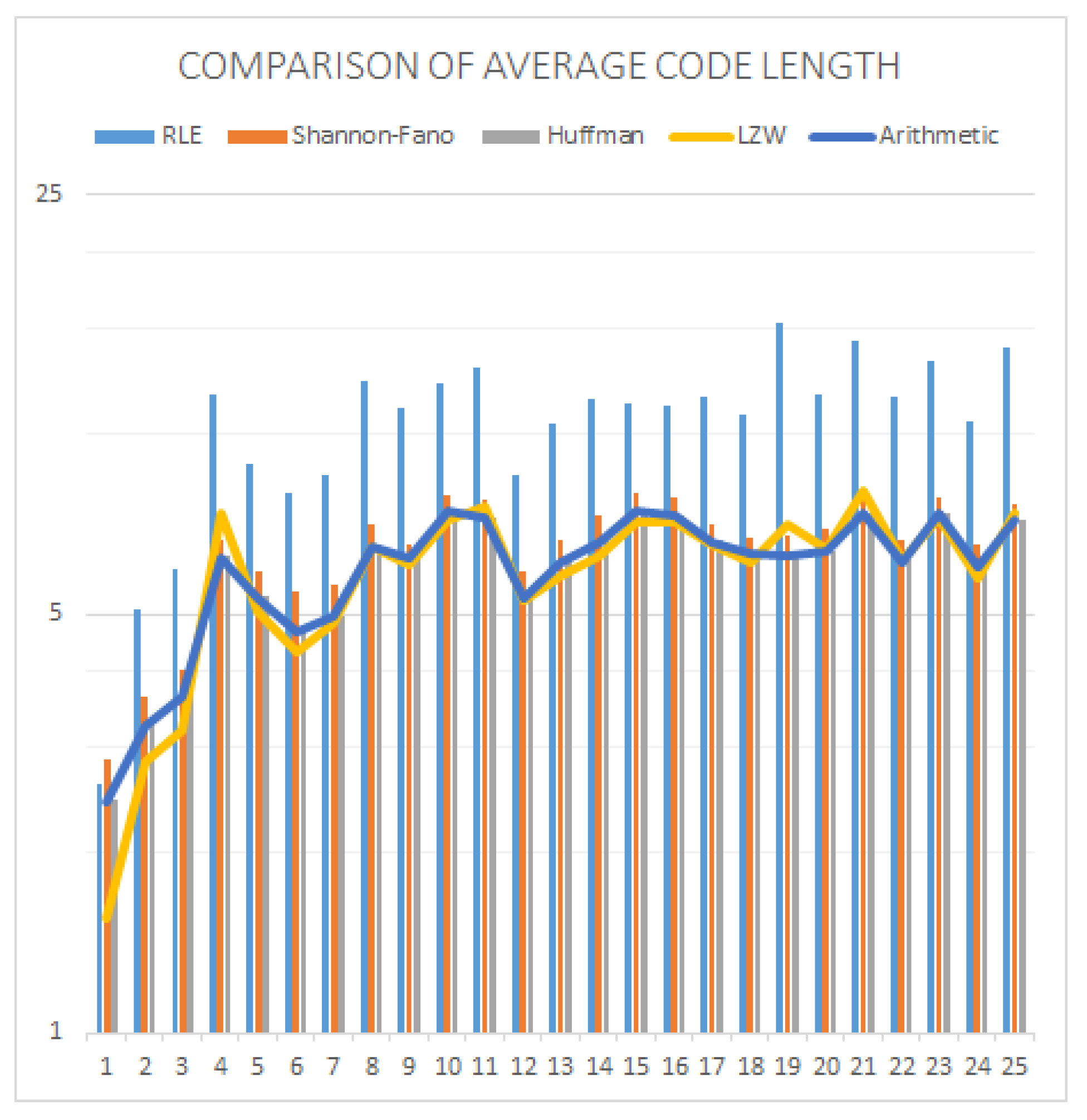
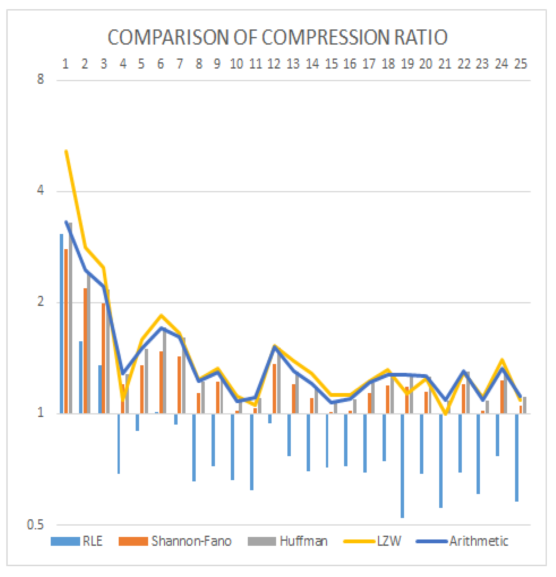
| Images | RLE | Shannon–Fano | Huffman | LZW | Arithmetic |
|---|---|---|---|---|---|
| 1 | 3.0635 | 2.7961 | 3.2795 | 5.1481 | 3.2969 |
| 2 | 1.5766 | 2.1924 | 2.4023 | 2.8237 | 2.451 |
| 3 | 1.3482 | 1.9825 | 2.1684 | 2.4966 | 2.2059 |
| 4 | 0.6889 | 1.2026 | 1.2813 | 1.0879 | 1.2849 |
| 5 | 0.9002 | 1.3551 | 1.4956 | 1.5903 | 1.5039 |
| 6 | 1.0075 | 1.4737 | 1.7085 | 1.8477 | 1.7123 |
| 7 | 0.935 | 1.425 | 1.6084 | 1.6506 | 1.615 |
| 8 | 0.6561 | 1.1364 | 1.2253 | 1.2387 | 1.2308 |
| 9 | 0.7222 | 1.2201 | 1.291 | 1.3231 | 1.2957 |
| 10 | 0.6595 | 1.0181 | 1.0772 | 1.1165 | 1.0815 |
| 11 | 0.622 | 1.0346 | 1.1008 | 1.0597 | 1.1057 |
| 12 | 0.9424 | 1.3589 | 1.5064 | 1.5236 | 1.5115 |
| 13 | 0.7705 | 1.201 | 1.3014 | 1.3878 | 1.3095 |
| 14 | 0.7011 | 1.1002 | 1.1876 | 1.2838 | 1.2104 |
| 15 | 0.7136 | 1.0081 | 1.0709 | 1.1259 | 1.0756 |
| 16 | 0.7204 | 1.0223 | 1.0916 | 1.1281 | 1.0959 |
| 17 | 0.6948 | 1.1337 | 1.2093 | 1.2241 | 1.2146 |
| 18 | 0.7436 | 1.1898 | 1.2664 | 1.3151 | 1.2721 |
| 19 | 0.5228 | 1.1798 | 1.2711 | 1.1326 | 1.2798 |
| 20 | 0.6896 | 1.1509 | 1.2562 | 1.2424 | 1.2607 |
| 21 | 0.5584 | 1.0216 | 1.0833 | 0.9977 | 1.0886 |
| 22 | 0.6932 | 1.2058 | 1.3033 | 1.3006 | 1.3083 |
| 23 | 0.6059 | 1.0198 | 1.0851 | 1.1081 | 1.0893 |
| 24 | 0.7652 | 1.2301 | 1.3212 | 1.3973 | 1.3305 |
| 25 | 0.577 | 1.0509 | 1.1135 | 1.0868 | 1.1191 |
| Average | 0.875128 | 1.30838 | 1.428224 | 1.545472 | 1.43798 |
© 2019 by the authors. Licensee MDPI, Basel, Switzerland. This article is an open access article distributed under the terms and conditions of the Creative Commons Attribution (CC BY) license (http://creativecommons.org/licenses/by/4.0/).
Share and Cite
Rahman, M.A.; Hamada, M. Lossless Image Compression Techniques: A State-of-the-Art Survey. Symmetry 2019, 11, 1274. https://doi.org/10.3390/sym11101274
Rahman MA, Hamada M. Lossless Image Compression Techniques: A State-of-the-Art Survey. Symmetry. 2019; 11(10):1274. https://doi.org/10.3390/sym11101274
Chicago/Turabian StyleRahman, Md. Atiqur, and Mohamed Hamada. 2019. "Lossless Image Compression Techniques: A State-of-the-Art Survey" Symmetry 11, no. 10: 1274. https://doi.org/10.3390/sym11101274
APA StyleRahman, M. A., & Hamada, M. (2019). Lossless Image Compression Techniques: A State-of-the-Art Survey. Symmetry, 11(10), 1274. https://doi.org/10.3390/sym11101274