Accurate Optic Disc and Cup Segmentation from Retinal Images Using a Multi-Feature Based Approach for Glaucoma Assessment

 ,
, 
Abstract
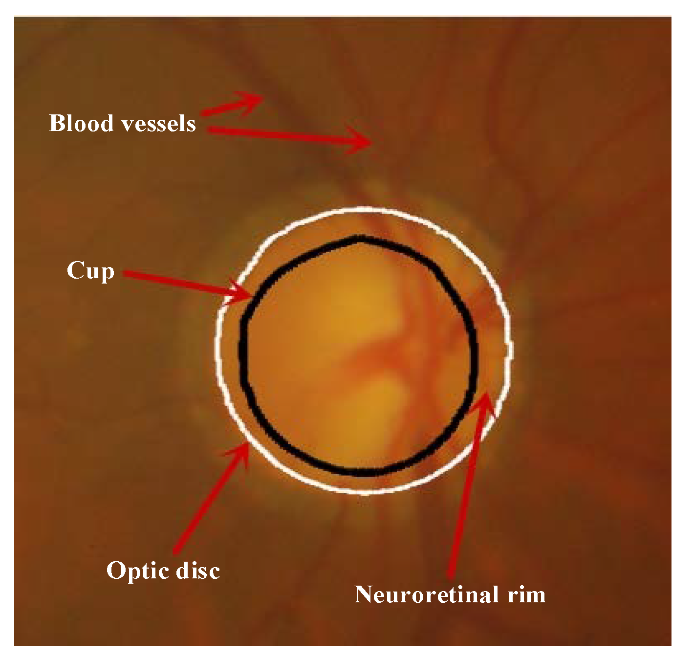
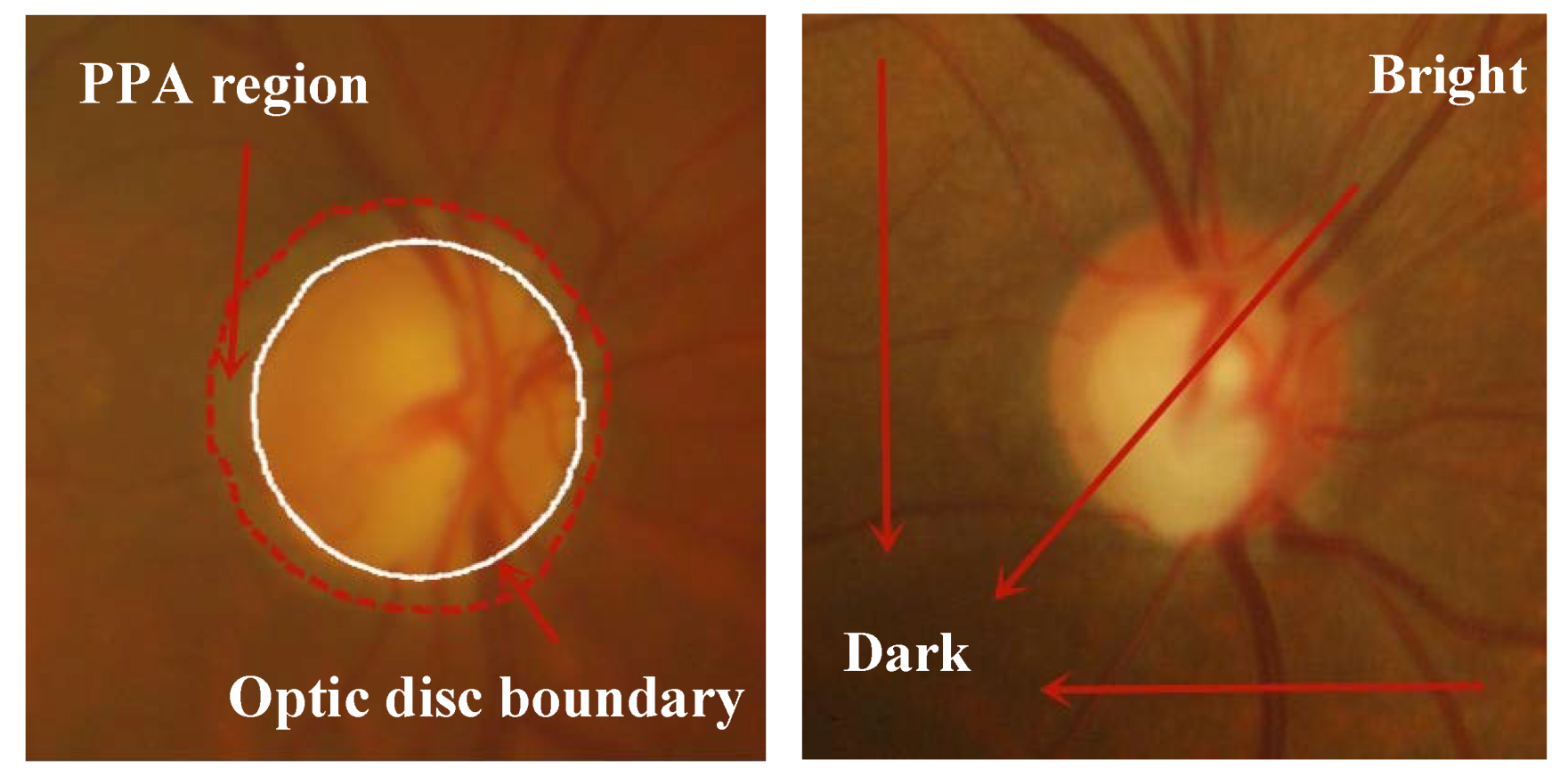
1. Introduction
2. Method
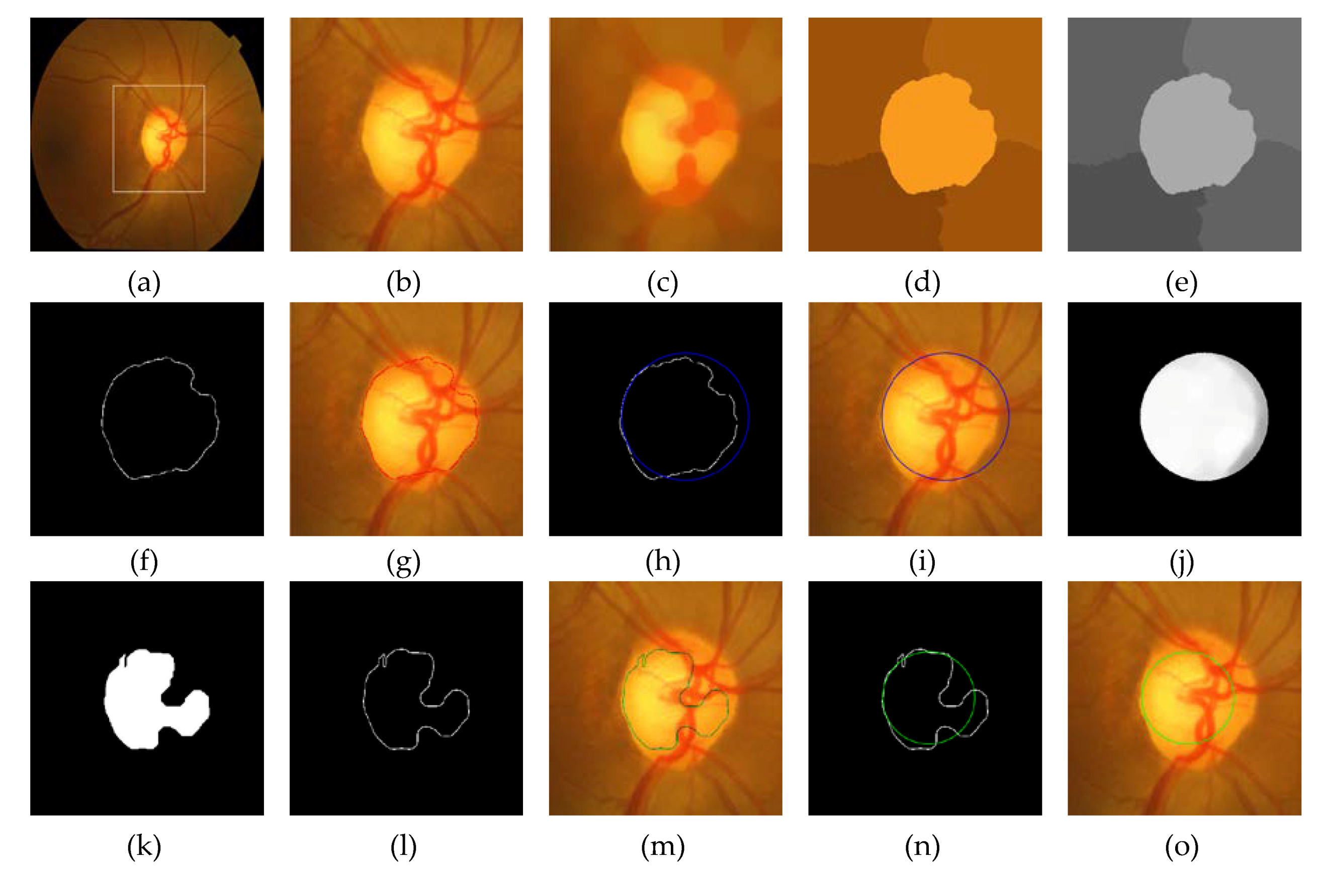
2.1. Rough Boundary Extraction
2.2. Accurate Boundary Curve Extraction of the OD
2.3. Accurate Boundary Curve Extraction of the OC
- Initialization: Input the set of multi-channel feature images including original red channel image, vessel-free red channel image, vessel-free green channel image, and value channel image from vessel-free HSV color space, , . The level set functions , . and are respectively initial level set function of the OD and the OC obtained in Section 2.1. and are respectively defined as iterations.
- Respectively update and , , , using (4)–(6).
- Evolve the level set functions, according to (7). If satisfies the stationary condition, stop; otherwise, and return to Step 2.
- Input level set function of the OD obtained in Step 3.
- Respectively update and , , , using (11)–(13).
- Evolve the level set functions, according to (14). If satisfies the stationary condition, stop; otherwise, and return to Step 5.
3. Experimental Results
3.1. Database
3.2. Evaluation Measures
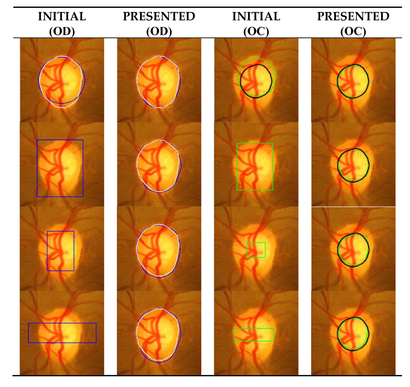
3.3. Segmentation Results with Different Initial Contour
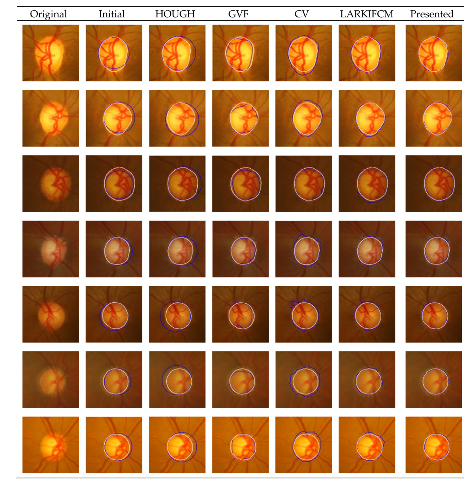
3.4. Optic Disc Segmentation Results
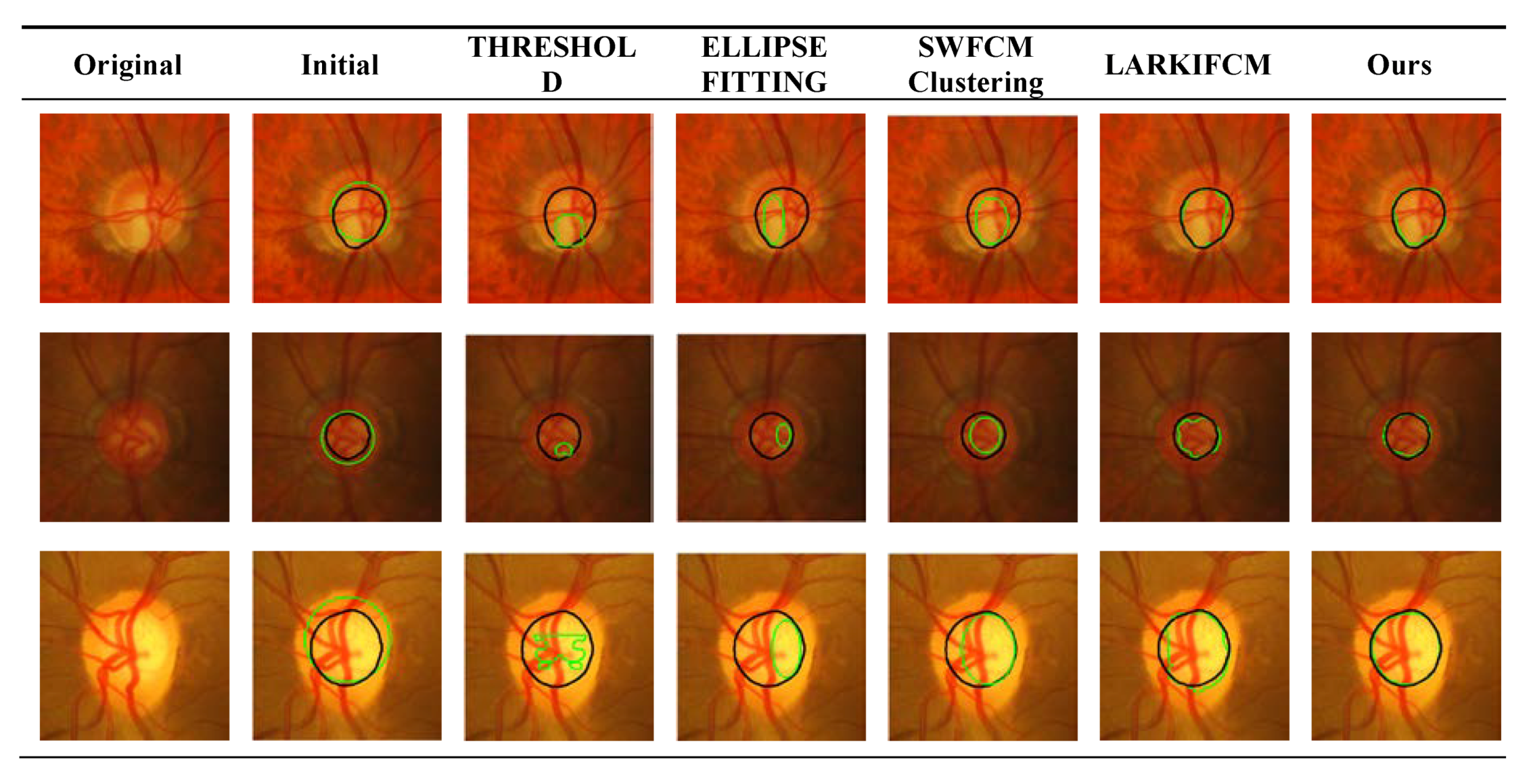
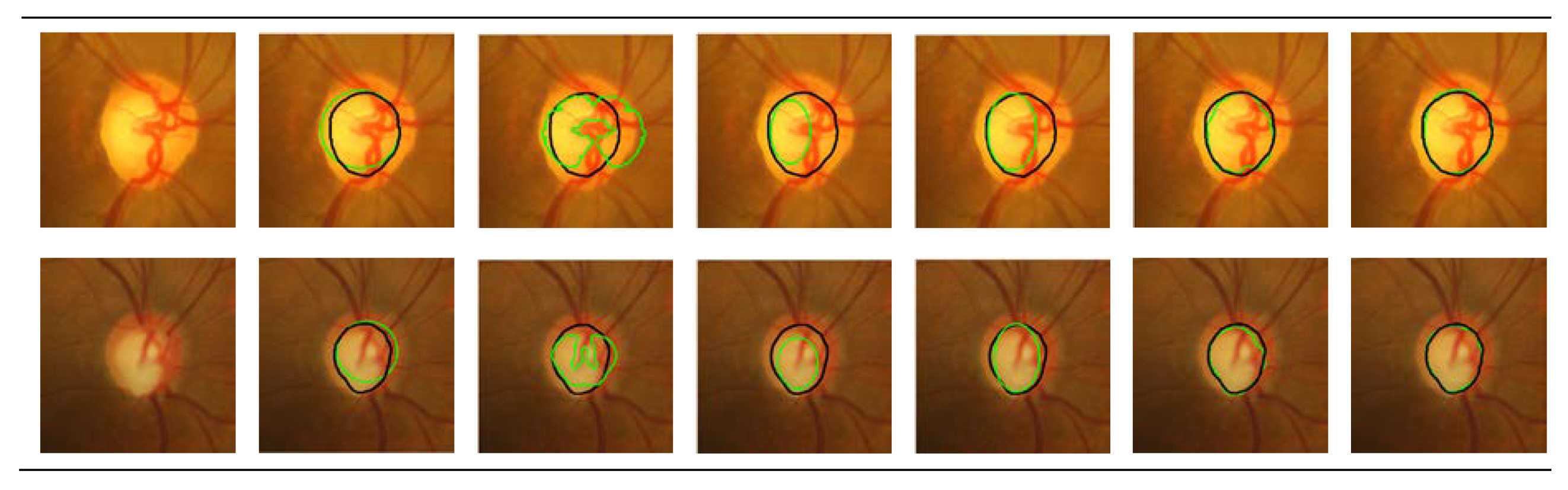
3.5. Optic Cup Segmentation Results
3.6. Glaucoma Assessment
4. Conclusions and Future Work
Author Contributions
Funding
Conflicts of Interest
References
- Lester, M.; Garway-Heath, D.; Lemij, H. Optic Nerve Head and Retinal Nerve Fibre Analysis; European Glaucoma Society: Editrice Dogma, Italy, 2005; pp. 121–149. [Google Scholar]
- Quigley, H.; Broman, A. The number of people with glaucoma worldwide in 2010 and 2020. Br. J. Ophthalmol. 2006, 90, 262–267. [Google Scholar] [CrossRef]
- Cheng, J.; Liu, J.; Xu, Y.; Yin, F.; Wong, D.; Tan, N. Superpixel classification based optic disc and optic cup segmentation for glaucoma screening. IEEE Trans. Med. Imaging 2013, 32, 1019. [Google Scholar] [CrossRef] [PubMed]
- Bock, R.; Meier, J.; Nyl, L.; Michelson, G. Glaucoma risk index: Automated glaucoma detection from color fundus images. Med. Image Anal. 2010, 14, 471–481. [Google Scholar] [CrossRef] [PubMed]
- Damms, T.; Dannheim, F. Sensitivity and specificity of optic disc parameters in chronic glaucoma. Invest. Ophth. Vis. Sci. 1993, 34, 2246–2250. [Google Scholar]
- Harizman, N.; Oliveira, C.; Chiang, A.; Tello, C.; Marmor, M.; Ritch, R.; Liebmann, J. The ISNT rule and differentiation of normal from glaucomatous eyes. Arch. Ophthalmol. 2006, 124, 1579–1583. [Google Scholar] [CrossRef] [PubMed]
- Pinz, A.; Bernogger, S.; Datlinger, P.; Kruger, A. Mapping the human retina. IEEE Trans. Med. Imaging 1988, 17, 606–619. [Google Scholar] [CrossRef] [PubMed]
- Li, H.; Chutatape, O. Automated feature extraction in color retinal images by a model based approach. IEEE Trans. Biomed. Eng. 2004, 51, 246–254. [Google Scholar] [CrossRef] [PubMed]
- Bhuiyan, A.; Kawasaki, R.; Wong, T.; Kotagiri, R. A new and efficient method for automatic optic disc detection using geometrical features. In Proceedings of the World Congress on Medical Physics and Biomedical Engineering, Munich, Germany, 7–12 September 2009; pp. 1131–1134. [Google Scholar]
- Aquino, A.; Gegúndez-Arias, M.; Marín, D. Detecting the optic disc boundary in digital fundus images using morphological, edge detection, and feature extraction techniques. IEEE Trans. Med. Imaging 2010, 29, 1860–1869. [Google Scholar] [CrossRef] [PubMed]
- Roychowdhury, S.; Koozekanani, D.; Kuchinka, S.; Parhi, K. Optic disc boundary and vessel origin segmentation of fundus images. IEEE J. Biomed. Health Inform. 2017, 20, 1562–1574. [Google Scholar] [CrossRef]
- Reza, A.; Eswaran, C.; Hati, S. Automatic tracing of optic disc and exudates from color fundus images using fixed and variable thresholds. J. Med. Syst. 2009, 33, 73–80. [Google Scholar] [CrossRef]
- Welfer, D.; Scharcanski, J.; Marinho, D. A morphologic two-stage approach for automated optic disk detection in color eye fundus images. Pattern Recognit. Lett. 2013, 34, 476–485. [Google Scholar] [CrossRef]
- Srivastava, R.; Cheng, J.; Wong, D.; Liu, J. Using deep learning for robustness to parapapillary atrophy in optic disc segmentation. In Proceedings of the 2015 IEEE 12th International Symposium on Biomedical Imaging, New York, NY, USA, 16–19 April 2015; pp. 768–771. [Google Scholar]
- Li, H.; Chutatape, O. Boundary detection of optic disk by a modified ASM method. Pattern Recognit. 2003, 36, 2093–2104. [Google Scholar] [CrossRef]
- Yin, F.; Liu, J.; Ong, S.; Sun, Y.; Wong, D.; Tan, N.; Cheung, C.; Baskaran, M.; Aung, T.; Wong, T. Model-based optic nerve head segmentation on retinal fundus images. In Proceedings of the International Conference of the IEEE Engineering in Medicine and Biology Society, Boston, MA, USA, 30 August–3 September 2011; pp. 2626–2629. [Google Scholar]
- Yin, F. Automated segmentation of optic disc and optic cup in fundus images for glaucoma diagnosis. In Proceedings of the 2012 25th IEEE International Symposium on Computer-Based Medical Systems (CBMS), Rome, Italy, 20–22 June 2012; pp. 1–6. [Google Scholar]
- Abràmoff, M.; Alward, W.; Greenlee, E.; Shuba, L.; Kim, C.; Fingert, J. Automated segmentation of the optic disc from stereo color photographs using physiologically plausible features. Investig. Ophthalmol. Visual Sci. 2007, 48, 1665–1673. [Google Scholar] [CrossRef] [PubMed]
- Dutta, M.; Mourya, A.; Singh, A.; Parthasarathi, M.; Burget, R.; Riha, K. Glaucoma detection by segmenting the super pixels from fundus colour retinal images. In Proceedings of the 2014 International Conference on Medical Imaging, m-Health and Emerging Communication Systems (Med Com), Greater Noida, India, 7–8 November 2014; pp. 86–90. [Google Scholar]
- Tan, N.; Xu, Y.; Goh, W.; Liu, J. Robust multi-scale superpixel classification for optic cup localization. Comput. Med. Imaging Graph. 2015, 40, 182–193. [Google Scholar] [CrossRef] [PubMed]
- Saeed, E.; Szymkowski, M.; Saeed, K.; Mariak, Z. An Approach to Automatic Hard Exudate Detection in Retina Color Images by a Telemedicine System Based on the d-Eye Sensor and Image Processing Algorithms. Sensors 2019, 19, 695. [Google Scholar] [CrossRef] [PubMed]
- Zhou, W.; Wu, C.; Chen, D.; Wang, Z.; Yi, Y.; Du, W. Automatic microaneurysm detection using the sparse principal component analysis based unsupervised classification method. IEEE Access 2017, 5, 2169–3536. [Google Scholar] [CrossRef]
- Zhou, W.; Wu, C.; Yi, Y.; Du, W. Automatic detection of exudates in digital color fundus images using superpixel multifeatured classification. IEEE Access 2017, 5, 17077–17088. [Google Scholar] [CrossRef]
- Mary, M.; Rajsingh, E.; Jacob, J. An empirical study on optic disc segmentation using an active contour model. Biomed. Signal Process. Control 2015, 18, 19–29. [Google Scholar] [CrossRef]
- Mendels, F. Identification of the optic disk boundary in retinal images using active contours. In Proceedings of the Irish Machine Vision and Image Processing Conference (IMVIP), Dublin, Ireland, 8–9 September 1999; pp. 103–115. [Google Scholar]
- Tang, Y.; Li, X.; von Freyberg, A.; Goch, G. Automatic segmentation of the papilla in a fundus image based on the C-V model and a shape restraint. In Proceedings of the 18th International Conference on Pattern Recognition (ICPR’06), Hong Kong, China, 20–24 August 2006; pp. 183–186. [Google Scholar]
- Wong, D.; Liu, J.; Lim, J. Level-set based automatic cup-to-disc ratio determination using retinal fundus images in ARGALI. In Proceedings of the 30th Annual International Conference of the IEEE Engineering in Medicine and Biology Society, Vancouver, BC, Canada, 20–25 August 2008; pp. 2266–2269. [Google Scholar]
- Yu, H.; Barriga, E.; Agurto, C.; Echegaray, S.; Pattichis, M.; Bauman, W.; Soliz, P. Fast localization and segmentation of optic disk in retinal images using directional matched filtering and level sets. IEEE Trans. Inf. Technol. Biomed. 2012, 16, 644–657. [Google Scholar] [CrossRef]
- Esmaeili, M.; Rabbani, H.; Dehnavi, A. Automatic optic disk boundary extraction by the use of curvelet transform and deformable variational level set model. Pattern Recognit. 2012, 45, 2832–2842. [Google Scholar] [CrossRef]
- Joshi, G.; Sivaswamy, J.; Karan, K.; Krishnadas, R. Optic disk and cup boundary detection using regional information. In Proceedings of the 2010 IEEE International Symposium on Biomedical Imaging: From Nano to Macro, Rotterdam, The Netherlands, 14–17 April 2010; pp. 948–951. [Google Scholar]
- Thakur, N.; Juneja, M. Optic disc and optic cup segmentation from retinal images using hybrid approach. Expert Syst. Appl. 2019, 127, 308–322. [Google Scholar] [CrossRef]
- Wong, D.; Liu, J.; Lim, J.; Li, H.; Jia, X.; Yin, F.; Wong, T. Automated detection of kinks from blood vessels for optic cup segmentation in retinal images. Proc. SPIE Med. Imaging 2009, 7260, 72601J. [Google Scholar]
- Liu, J.; Wong, D.; Lim, J.; Li, H.; Tan, N.; Wong, T. Argali—An automatic cup-to-disc ratio measurement system for glaucoma detection and analysis framework. Proc. SPIE Med. Imaging 2009, 7260, 72603K. [Google Scholar]
- Mittapalli, P.; Kande, G. Segmentation of optic disk and optic cup from digital fundus images for the assessment of glaucoma. Biomed. Signal Process. Control 2016, 24, 34–46. [Google Scholar] [CrossRef]
- Li, C.; Huang, R.; Ding, Z.; Gatenby, C.; Metaxas, C.; Gore, J. A level set method for image segmentation in the presence of intensity inhomogeneities with application to MRI. IEEE Trans. Image Process. 2011, 20, 2007–2016. [Google Scholar] [PubMed]
- Wang, L.; Li, C.; Sun, Q.; Xia, D.; Kao, C. Active contours driven by local and global intensity fitting energy with application to brain MR image segmentation. Comput. Med. Imaging Graph. 2009, 33, 520–531. [Google Scholar] [CrossRef]
- Li, C.; Kao, C.; Gore, J.; Ding, Z. Implicit active contours driven by local binary fitting energy. In Proceedings of the 2007 IEEE Conference on Computer Vision and Pattern Recognition, Minneapolis, MN, USA, 17–22 June 2007; pp. 1–7. [Google Scholar]
- Zhou, W.; Wu, C.; Gao, Y.; Yu, X. Automatic optic disc boundary extraction based on saliency object detection and modified local intensity clustering model in retinal images. IEICE Trans. Fundam. 2017, E100-A, 2069–2072. [Google Scholar] [CrossRef]
- Comaniciu, D.; Meer, P. A robust approach toward feature space analysis. IEEE Trans. Pattern Anal. Mach. Intell. 2002, 24, 603–619. [Google Scholar] [CrossRef]
- Liu, J.; Wong, D.; Lim, J.; Jia, X. Optic cup and disk extraction from retinal fundus images for determination of cup-to-disc ratio. In Proceedings of the IEEE Conference on Industrial Electronics and Applications, Singapore, 3–5 June 2008; pp. 1828–1832. [Google Scholar]
- Sivaswamy, J.; Krishnadas, S.; Joshi, G.; Jain, M.; Tabish, A. Drishti-GS: Retinal image dataset for optic nerve head (ONH) segmentation. In Proceedings of the 2014 IEEE 11th International Symposium on Biomedical Imaging (ISBI), Beijing, China, 29 April–2 May 2014; pp. 53–56. [Google Scholar]
- Chr´astek, R.; Wolf, M.; Donath, K.; Michelson, G.; Niemann, H. Optic disc segmentation in retinal images. In Bildverarbeitung für die Medizin; Springer-Verlag: Berlin, Germany, 2002; pp. 263–266. [Google Scholar]
- Osareh, A.; Mirmehdi, M.; Thomas, B.; Markham, R. Colour morphology and snakes for optic disc localization. In Proceedings of the 6th Medical Image Understanding and Analysis Conference, Portsmouth, UK, 22–23 July 2002; pp. 21–24. [Google Scholar]
- Joshi, G.; Sivaswamy, J.; Krishnadas, S. Optic disk and cup segmentation from monocular color retinal images for glaucoma assessment. IEEE Trans. Med. Imaging 2011, 30, 1192–1205. [Google Scholar] [CrossRef]


| Methods | F-Score for OD (Average) | Boundary-Based Distance for OD (Average) | F-Score for OC (Average) | Boundary-Based Distance for OC (Average) |
|---|---|---|---|---|
| Contour intersecting the OD or OC | 0.942 | 9.521 | 0.813 | 23.213 |
| Contour within the OD or OC | 0.944 | 9.281 | 0.815 | 23.152 |
| Contour outside the OD or OC | 0.945 | 9.162 | 0.818 | 22.965 |
| Adaptive contour | 0.947 | 8.885 | 0.826 | 21.980 |
| Methods | F-Score (Average) | Boundary-Based Distance (Average) |
|---|---|---|
| Hough [42] | 0.836 | 43.126 |
| GVF [43] | 0.862 | 39.561 |
| C-V [30] | 0.881 | 27.578 |
| LARKIFCM [31] | 0.940 | 9.882 |
| Ours | 0.947 | 8.885 |
| Method | F-Score (Average) | Boundary-Based Distance (Average) |
|---|---|---|
| Thresholding [30] | 0.616 | 51.347 |
| Ellipse Fitting [33] | 0.651 | 48.799 |
| SWFCM Clustering [34] | 0.765 | 27.376 |
| LARKIFCM [31] | 0.811 | 23.335 |
| Ours | 0.826 | 21.980 |
| Retinal Image | Cup-to-Disc Vertical Diameter Ratio | Cup-to-Disc Area Ratio | ||
|---|---|---|---|---|
| μError | σError | |||
| Normal Images (31) | 0.158 | 0.104 | 0.172 | 0.127 |
| Glaucoma Images (70) | 0.095 | 0.084 | 0.101 | 0.091 |
| Total Images (101) | 0.110 | 0.099 | 0.118 | 0.119 |
© 2019 by the authors. Licensee MDPI, Basel, Switzerland. This article is an open access article distributed under the terms and conditions of the Creative Commons Attribution (CC BY) license (http://creativecommons.org/licenses/by/4.0/).
Share and Cite
Gao, Y.; Yu, X.; Wu, C.; Zhou, W.; Wang, X.; Zhuang, Y. Accurate Optic Disc and Cup Segmentation from Retinal Images Using a Multi-Feature Based Approach for Glaucoma Assessment. Symmetry 2019, 11, 1267. https://doi.org/10.3390/sym11101267
Gao Y, Yu X, Wu C, Zhou W, Wang X, Zhuang Y. Accurate Optic Disc and Cup Segmentation from Retinal Images Using a Multi-Feature Based Approach for Glaucoma Assessment. Symmetry. 2019; 11(10):1267. https://doi.org/10.3390/sym11101267
Chicago/Turabian StyleGao, Yuan, Xiaosheng Yu, Chengdong Wu, Wei Zhou, Xiaonan Wang, and Yaoming Zhuang. 2019. "Accurate Optic Disc and Cup Segmentation from Retinal Images Using a Multi-Feature Based Approach for Glaucoma Assessment" Symmetry 11, no. 10: 1267. https://doi.org/10.3390/sym11101267
APA StyleGao, Y., Yu, X., Wu, C., Zhou, W., Wang, X., & Zhuang, Y. (2019). Accurate Optic Disc and Cup Segmentation from Retinal Images Using a Multi-Feature Based Approach for Glaucoma Assessment. Symmetry, 11(10), 1267. https://doi.org/10.3390/sym11101267