Improving Human Motion Classification by Applying Bagging and Symmetry to PCA-Based Features

Abstract

This paper proposes a method for improving human motion classification by applying bagging and symmetry to Principal Component Analysis (PCA)-based features. In contrast to well-known bagging algorithms such as random forest, the proposed method recalculates the motion features for each “weak classifier” (it does not randomly sample a feature set). The proposed classification method was evaluated on a challenging (even to a human observer) motion capture recording dataset of martial arts techniques performed by professional karate sportspeople. The dataset consisted of 360 recordings in 12 motion classes. Because some classes of these motions might be symmetrical (which means that they are performed with a dominant left or right hand/leg), an analysis was conducted to determine whether accounting for symmetry could improve the recognition rate of a classifier. The experimental results show that applying the proposed classifiers’ bagging procedure increased the recognition rate (RR) of the Nearest-Neighbor (NNg) and Support Vector Machine (SVM) classifiers by more than 5% and 3%, respectively. The RR of one trained classifier (SVM) was higher when we did not use symmetry. On the other hand, the application of symmetry information for bagged NNg improved its recognition rate compared with the results without symmetry information. We can conclude that symmetry information might be helpful in situations in which it is not possible to optimize the decision borders of the classifier (for example, when we do not have direct information about class labels). The experiment presented in this paper shows that, in this case, bagging and mirroring might help find a similar object in the training set that shares the same class label. Both the dataset that was used for the evaluation and the implementation of the proposed method can be downloaded, so the experiment is easily reproducible.

1. Introduction

Human motion analysis and recognition are among the most interesting and challenging applications of digital signal processing and classification. Depending on the motion capture (MoCap) technique, human activities are measured either by a set of time-varying positions of body joints in 3D space or a set of 3D rotations of the joints with a fixed distance between particular joints. In the second case, the set of vectors with fixed lengths that show the dependence of the spatial positions of the joints (joint hierarchy, also called a kinematic chain) is called a skeleton. Of course, it is possible to recalculate one of the previously mentioned motion representations to another. Modern vision-based and IMU-based (internal measurement units) motion capture hardware [1] enables precise measurement of the human body’s spatial position with a high-frequency rate and can be applied in many fields of science and industry, such as medicine and rehabilitation [2], computer graphics [3], and robotics [4]. Many institutions prepare their own private or publicly available databases that contain recordings of various human activities. When a database becomes large, there is a need to search these databases in order to find similar types of motions. To determine whether signals are similar, one has to define a metric that allows for the expression of similarity, preferably as a single real, non-negative value.

1.1. Challenges in Human Motion Comparison and Classification

Several factors make direct MoCap signal comparison a difficult task. Among the most important factors is the fact that the same types of motions can be performed at different speeds. Furthermore, people might differ in their flexibility, which causes variation in motion ranges. Additionally, people in the recordings might face different directions and perform the same motions in different planes (if the motions have a dominant plane of displacement). It should also be recalled that MoCap technology acquires data at a high frequency (80 Hz or more) as it registers the motions of many body parts simultaneously. For this reason, there are dozens of data samples that describe each motion frame and thousands of data samples for a whole motion sequence. The motion of each separate body joint is described by a multidimensional time-varying function. This description is either a three-dimensional position in space or a rotation angle in a kinematic chain: a three-dimensional vector of Euler angles or a four-dimensional vector of the quaternion. Finally, some motions might be very similar to each other; for example, recordings of martial arts techniques contain several types of blocks, kicks, and punches that have basically the same initial and final stands (starting and ending body positions) that differ only in the trajectories of the selected joints.

All these factors make motion compression and classification challenging and limit the number of techniques that can be successfully applied. Among the most important factors to overcome is a large number of motion features because it makes a direct frame-by-frame comparison of two motions inefficient. One of the most successful methods of feature selection that is discussed in this paper applies Principal Component Analysis (PCA).

1.2. Recent Work in the Application of PCA for Human Motion Analysis

The PCA-based representation of human faces has a well-known name (the eigenfaces algorithm [5]), but a similar technique for motion capture is reported with various names, or the authors do not mention the name at all. For example, in [6], the authors used so-called eigensequences. They defined the initial feature space using only angular data from a hierarchical kinematic model (however, they did not account for the singularities of Euler angles). In this model, motions are split into “atomic” motions, which are the objects of PCA. In [7], the authors created so-called signatures, which were PCA-compressed 3D trajectories of motions of a multimedia Wii controller. The authors of [8] performed a classification of motion patterns in fencing kinematic data. In consideration of the reliability of analyzing joint angles (the empirical observations and the PCA results), the authors used only coordinate variables of the arm and the lower limbs. In [9,10], the authors described a process for distinguishing a single class of motions from others using a combination of 11 various angles and distance-based features, which were compressed by PCA and then classified by Support Vector Machine (SVM). For the purpose of gait recognition, the authors of [11] performed PCA on six-dimensional data, which consisted of the left and right thigh angles, the inter-thigh angle, the inter-thigh angular velocity, the left knee angle, and the left knee angular velocities. Utilizing angular motion descriptions, the authors of [12] described a procedure for diagnosing motion pathologies on the basis of PCA-reduced kinematical data on gait. In [13], the authors used PCA to compare skilled and novice groups to determine the number of components required to account for the variance of aiming while on a force platform. In [14], the authors also compared the skill levels of participants using PCA dimensionality reduction, but they analyzed juggling actions. In [15], PCA was applied to compare lower-body kinematics during loaded walking compared with unloaded walking. The authors of [16] used PCA to reduce the feature space in the kinematic analysis of gait while the participants adapted to variable and asymmetric split-belt treadmill walking. In [17], radial basis functions (RBFs) and PCA were used to model and extract stylistic and affective features from motion data. The authors of [18] also described PCA as an important linear dimensionality reduction technique for MoCap.

A different approach for similar action retrieval (not strictly classification) was presented in [19], in which PCA was carried out on a set of motion frames rather than the whole motion (they used displacement data as the initial feature space). Then, the compressed motion data were divided into similar postures by using k-means clustering. Each motion in the database was a composition of those clustered fragments. In [20], the authors used PCA to minimize the feature space by taking into account each angle-based feature separately.

Besides classification, authors have reported using PCA-based features for walking motion synthesis [3,21,22], motion segmentation [23], keyframe extraction [24], mapping MoCap data to a servos system of a humanoid robot [4] (the authors named their approach Eigenposes), compensating for the effect of sensor position changes during a MoCap session [25], and the synchronization of motion sequences from different sources [26].

All the popular algorithms mentioned above use two main types of features derived from MoCap recordings that are later processed by PCA: three-dimensional trajectories of body joints approximated by MoCap marker positions [7,13,14,19] or angle-based features [6,8,9,10,11,12,15,20]. The number of features that are used for further processing depends on the motion capture hardware and the parts of the body that are analyzed. The analysis may consider an example of full-body motion, lower-limb kinematics, or the motion of a handheld device. After feature selection and calculation, authors often use well-known classifiers, such as SVM.

1.3. Contributions of This Research

This paper proposes the application of PCA, together with classifier bagging, for the generation of motion features [27]. In contrast to well-known bagging algorithms such as random forest, the proposed method recalculates motion features for each “weak classifier” (it does not randomly sample a feature set).

To date, the approach proposed in this paper has not been evaluated in recently published papers.

The proposed classification method was evaluated on a challenging (even to a human observer) motion capture recording dataset of martial arts techniques performed by professional karate sportspeople. The dataset consists of 360 recordings in 12 motion classes. Because some classes of these motions might be symmetrical (which means that they are performed with a dominant left or right hand/leg), an analysis was performed to determine whether accounting for symmetry could improve the recognition rate of a classifier.

To the best of the author’s knowledge, the application of symmetry to improve the recognition rate of motion capture data has not been evaluated yet.

The results obtained by applying information about symmetry for the augmentation of the training dataset [28] were compared. The proposed approach was validated on linear and nonlinear classifiers, namely, the Nearest-Neighbor classifier (NNg) and Support Vector Machine (SVM) with three types of kernels (linear, sigmoid, and radial). Both the dataset that was used for evaluation and the implementation of the proposed method can be downloaded, so the experiment is easily reproducible (see [29]).

2. Materials and Methods

This section describes the MoCap dataset that was used to conduct the experiment, the feature space definition, and the classification algorithm.

2.1. Dataset

The MoCap data used in this study were recorded with a Shadow 2.0 wireless motion capture system, which consists of 17 inertial measurement units that contain a three-axis accelerometer, gyroscope, and magnetometer. The tracking frequency was set to 100 Hz with 0.5 degrees of static accuracy and 2 degrees of dynamic accuracy.

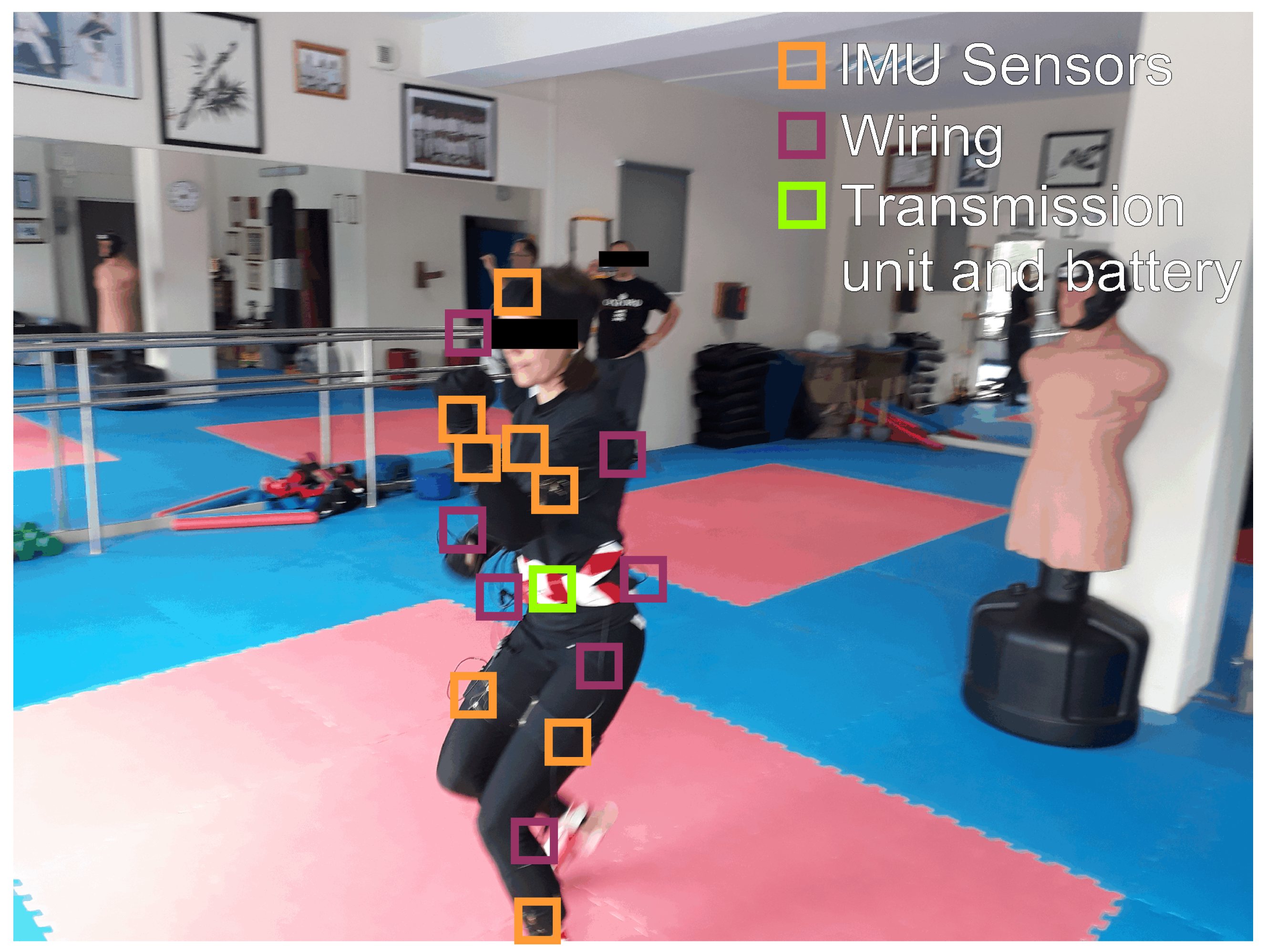
Data were collected in a dojo (training room) of a karate club. The environment was free of electromagnetic disturbances that could potentially affect the recordings. The persons taking part in the recording wore elastic clothing, to which the MoCap system was attached (see Figure 1). IMUs were attached either to a special vest or to elastic straps. The sensors were wired to a transmission unit that had a WiFi router. The sensor positions on the body were the same as those in [30]. The transmission unit and its battery were positioned on the waist. The data recorded during the session were transmitted via WiFi in real time to a dedicated application (Motion Monitor) that was installed on a laptop. With the Shadow system API (application programming interface), it was possible to convert the data from the raw format to BVH file format. The BVH files were used in this research.

All persons taking part in the experiment were volunteers. The physical effort exerted by the participants during the motion capture session did not exceed the karate training that the they typically underwent. All physical exercises were performed with the presence of a certificated karate trainer. They performed proper warm-up, thus the risk of injury was minimal. Prior to the experiment, they were introduced to the project and informed of their rights. They also had access to the data that were collected and were able to end the MoCap session at any time. The acquired data were stored anonymously. The author of this paper received anonymized MoCap data that could not be combined with other reasonably available information to identify individuals (The source of the data is http://gdl.org.pl/). For this reason, this research does not fall into the category of human subject research.

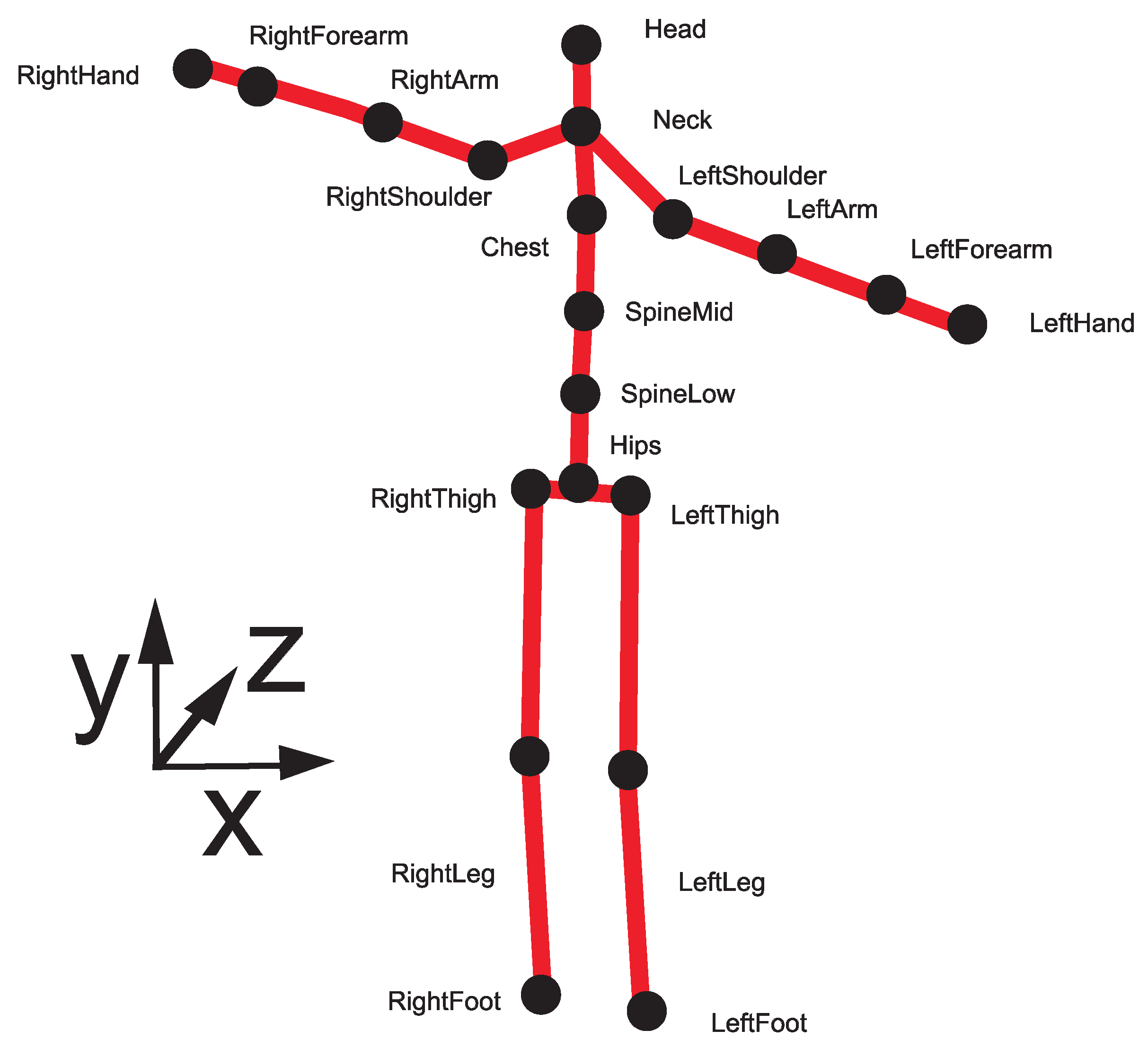
A detailed description of system calibration and the recording protocol can be found in [30]. The MoCap system-produced skeleton consisted of 20 body joints, as presented in Figure 2.

The dataset that was used in this research contains recordings of three professional Shorin-ryu karate sportspersons (world and national medalists) with many years of experience. All of them were male with different ages and body proportions. Each participant performed the following 12 types of karate techniques and each technique was repeated 10 times:

• blocks: age uke with the left hand, age uke with the right hand, gedan barai with the left hand, gedan barai with the right hand;
• strikes: empi with the left elbow, empi with the right elbow; and
• kicks: hiza geri with the left knee, hiza geri with the right knee, mae geri with the left leg, mae geri right with the right leg, yoko geri with the left leg, yoko geri with the right leg.

The detailed movement descriptions with illustrations can be found, for example, in [31]. There are a total of 360 motion recordings with 12 classes. It is apparent that the number of classes is not much greater than the number of exemplar recordings of each class. This situation is not typical for machine learning algorithms but is common for MoCap datasets since one prefers to store fewer high-quality recordings of top sportspeople than many recordings of less-skilled athletes. Furthermore, a karate technique dataset is among the hardest to classify because all recordings start and end in the same initial stance (zenkutsu dachi). To an amateur observer, the limb trajectories of the individuals while they perform the attacks are quite similar. Additionally, skilled athletes try to perform the initial parts of the attacks (for example, kicks) in a similar manner in order to throw off their opponent. Just before hitting the opponent, they choose the desired attack. This is especially visible during kicking, for which the initial parts are the same for all types. As a result, techniques such as mae geri and hiza geri are hard to distinguish from each other, even though mae geri is a frontal kick, whereas the impact during hiza geri is performed from sideways position.

There are also factors that can potentially improve the machine learning results: each motion in the dataset was performed with both the left and right dominant side. Therefore, in some recordings, symmetry in the dataset might be a potential factor that can be used to augment the dataset. Dataset augmentation refers to the enlargement of the training dataset to overcome overfitting by the classifier [28].

All recorded motions, except for yoko geri (side kick), could be correctly performed by a person with less training experience than that of the athletes who took part in the MoCap session. Yoko geri is the exception because it requires flexibility of the hips that might not be feasible for an untrained person. The karate dataset was chosen for evaluation because karate techniques are well-defined action classes that use various body parts simultaneously. The choice of the dataset does not make the proposed classifier less applicable to “real-world” (non-athlete/non-professional) settings.

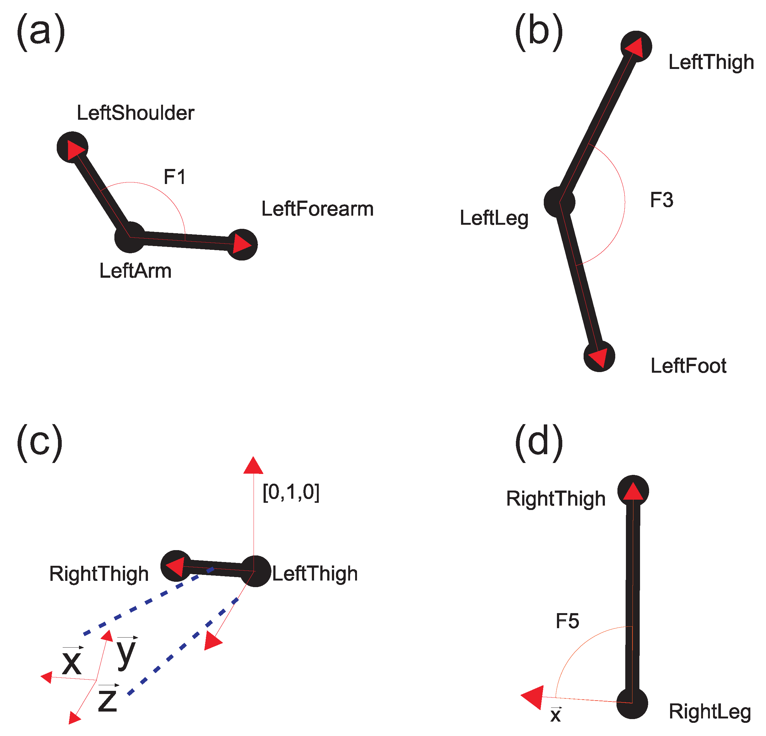
2.2. Feature Space Definition

Each MoCap recording in the dataset presented in the previous section consists of a set of time series of 3D rotations defined for each body joint and the translation of the root joint; this is is a hierarchical motion description. In the proposed feature selection method, the hierarchical model is recalculated to a direct kinematic model in order to obtain the spatial positions of each body joint. In the next step, all MoCap recordings are rescaled so that they have the same length (in this research, FMM spline was used [32]). Then, the new set of angle-based features is defined. This feature set is a combination of local planar rotation angles and global planar rotation angles. The angle between two vectors is calculated according to Equation (1) (see Equations (A1)–(A3) in the Appendix A for details).

$$\measuredangle \overrightarrow{v_i},\overrightarrow{v_j}=\left\{\begin{array}{ccc}2·asin\left(\frac{\overrightarrow{v_i}-\overrightarrow{v_j}}{2·\left|\overrightarrow{v_i}-\overrightarrow{v_j}\right|}\right)& \mathrm{if}& \overrightarrow{v_i}\circ \overrightarrow{v_j}\ge 0\\ \pi -2·asin\left(\frac{-\overrightarrow{v_i}-\overrightarrow{v_j}}{2·\left|-\overrightarrow{v_i}-\overrightarrow{v_j}\right|}\right)& \mathrm{if}& \overrightarrow{v_i}\circ \overrightarrow{v_j}<0\end{array}\right.$$

(1)

A similar but limited feature set was successfully used in other studies [33,34]. The 28-dimensional feature set in the present study has important advantages over a hierarchical model. The proposed feature set does not contain singularities, which occur very often with the use of Euler angle descriptions, and it does not use normalized quaternions, which are quite impractical for PCA-based analysis. Additionally, the proposed method is very intuitive; for example, $F_{1t},F_{2t}$ (t is an index of the sample) are flexion movements of the elbows, and $F_{3t},F_{4t},F_{1t},F_{2t}$ are flexion movements of the knees. The global coordinate frame in Equation (A2) is defined by a vector that links the left and right thigh in the first frame of MoCap ($t=1$), the up vector [0,1,0], and the appropriate vector product between them. Then, the coordinates’ frame vectors in Equation (A2) are used to calculate the angles between them and the body parts. For example, $\overrightarrow{(RightThig{h}_t-RightLe{g}_t)}$ is a vector that defines the direction of the right thigh, and $\overrightarrow{(RightShoulde{r}_t-RightAr{m}_t)}$ defines the direction of the right arm. Each of the 28 features is calculated for each MoCap acquisition frame. Each motion is described using $n·l$ values, where n is the number of features, and l is the number of acquisition frames. The disadvantage of this feature set is that it does not take into account all possible motions that might appear in the dataset (for example, wrist rotations). However, the experiment was not designed to examine motions on such low granularity, and if one wanted to examine such types of motions, the feature model could be easily extended to cover it.

In the next section, a method for PCA-based feature generation is presented.

2.3. Applying PCA for MoCap Feature Generation

Motion data are processed by PCA in a very similar manner to the face recognition procedure for the eigenfaces technique [5] (see Figure 3).

First, one has to generate the appropriate initial vectors of features for each MoCap recording (see Equations (A1)–(A3)). All of them have the same length. As previously mentioned, the length equals $n·l$ in this case. Let us assume that we have m MoCap recordings in the training set. Then, matrix D is created in which the columns contain vectors of feature values that are ordered one by one. This means that each column corresponds to a single MoCap recording from the training dataset (see the layout of matrix D in Figure 3). Then, a mean vector $\overrightarrow{m_F}$ of the rows of matrix D is calculated. This means that each coordinate of vector $\overrightarrow{m_F}$ contains the mean value of the particular feature calculated from the training dataset. Next, we have to subtract $\overrightarrow{m_F}$ from each motion description in D (indexes near the selected matrix symbols show the dimensionality of each object):

$$\begin{array}{c}{D}_{n·l\times m}^{\prime }=D_{n·l\times m}-{\left[\left|\overrightarrow{m_F}\right|\left|\overrightarrow{m_F}\right|⋮\left|\overrightarrow{m_F}\right|\right]}_{n·l\times m}\end{array}$$

(2)

A covariance matrix A is calculated using $D^{\prime }$:

$$\begin{array}{c}A:=cov\left(D^{\prime }\right)\end{array}$$

(3)

Then, we find k eigenvectors $[\overrightarrow{x_1},\dots ,\overrightarrow{x_k}]$ (they are organized in the columns of matrix X) that correspond to the k eigenvalues $\overrightarrow{\lambda }=[{\lambda }_1,\dots ,{\lambda }_k]$ with the highest value (the covariance matrix is symmetric and real, so eigenvalues are real and positive):

$$X={\left[\left|\overrightarrow{x_1}\right|\left|\overrightarrow{x_2}\right|⋮\left|\overrightarrow{x_k}\right|\right]}_{n\times k}$$

(4)

The cumulative sums of variance explained by i features are

$$v_{\%i}=1-\frac{{\lambda }_i}{{\sum }_{j=1}^k{\lambda }_j}$$

(5)

Next, matrix $D^{\prime }$ is projected onto k-dimensional space by performing the following matrix multiplication:

$$D_F={\left[\left|{\overrightarrow{\lambda }}^T\right|⋮\left|{\overrightarrow{\lambda }}^T\right|\right]}_{k\times k}·(X^T·D^{\prime })$$

(6)

After the above operation, matrix $D_F$ contains the features of all MoCap recordings from the training dataset in k-dimensional vectors. We can also use matrix X to project any $\overrightarrow{m_i}$ vector with the length $n·l$ onto k-dimensional space. In practice, this means recalculating the $n·l$-length vector MoCap representation to a k-length vector representation.

$$\begin{array}{c}\overrightarrow{m_{iF}}={\overrightarrow{\lambda }}^T·(X^T·(\overrightarrow{m_i}-\overrightarrow{m_F}))\end{array}$$

(7)

In essence, the new MoCap recording representation is a linear combination of eigenvectors that are in matrix X.

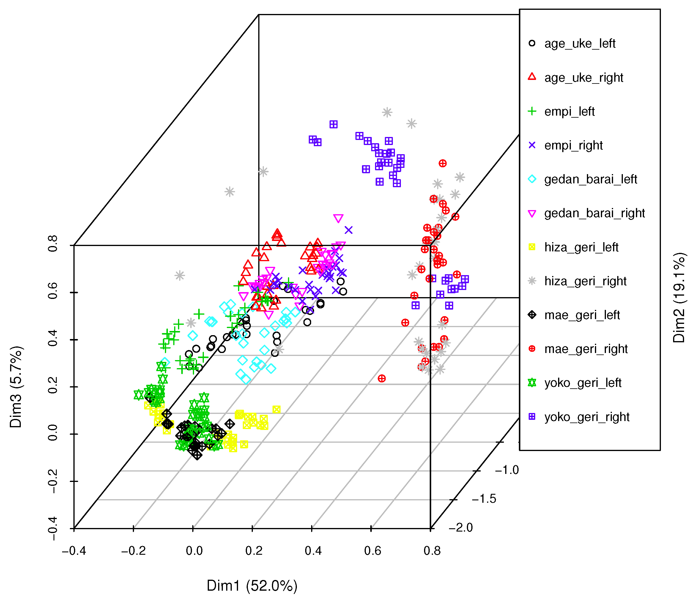
The projection of the whole dataset from Section 2.1 onto 3D space is presented in Figure 4. As shown in the figure, although the first three dimensions explain $76.8\%$ of the variance, objects of certain classes are situated very close to one another. For example, yoko geri and hiza geri kicks are close to each other, as are gedan barai and empi (the Euclidean distances between the exemplars of those classes are relatively small, and they seem to be mixed with each other; they do not create homogeneous clusters). Further, the distribution of objects of a single class is neither concentric nor uniform in density (see, for example, yoko geri right class). This suggests that three dimensions are not enough to model the variety in the dataset. It might also be possible that a single classifier trained on a whole training dataset is not capable of describing all the distinguishable objects. In the next section, the proposed classifier bagging algorithm for application to motion capture data is discussed.

The object distribution in the feature space might differ depending on the motion classes that we want to analyze and the feature set that was applied; however, the PCA projection that is presented in Figure 4 should always be performed as the initial step of multidimensional data analysis and classification. When the set meant to be classified is labeled (as in this dataset), we can judge the complexity of the problem by visually analyzing the positioning of the objects in the space and the class distribution in the same manner in which this MoCap dataset was assessed.

2.4. Classifier Bagging

As observed in Section 1.2, classifier bagging is not used for PCA features. This is because PCA is already a dimensionality reduction technique that takes advantage of the correlation between input features, thus it reduces the dimensional complexity of the problem. On the other hand, taking a subset of PCA features as a “weak classifier” in the bagging schema is invalid because the data might lose dimensions that are responsible for high variance in the data. The only reasonable method for applying bagging to the data on which one intends to perform PCA is to carry it out before PCA. This can be done by selecting a subset of input features or a subset of classes (or both). While performing PCA, we want to strengthen the influence of features with high variance, so there is no point in randomly removing some relevant features from the dataset. In sum, bagging should be performed on objects of a random subset of classes. Those random subsets of the training dataset should be used to train “weak classifiers”. The formal definition of the proposed classifier bagging procedure for MoCap data is

$$B_{C,p}:=\left\{\begin{array}{c}{w}_{1R{\left(C\right)}_1}\\ ⋮\\ w_{pR{\left(C\right)}_p}\end{array}\right.$$

(8)

where $B_C$ is a classifier that performs bootstrap aggregating (bagging) using p “weak classifiers” that were trained on set C; $w_{1R{\left(C\right)}_1}$ is the first “weak classifier” that was trained on a random subset of objects of C (called $R{\left(C\right)}_1$); and $w_p$ is the pth “weak classifier” that was trained on a random subset of objects of C, namely, $R{\left(C\right)}_p$.

Random selection was performed on class labels without replacement. For example, for 12 classes and a subset size of 10, we took all objects of 10 random classes (without replacement) so that all the objects of two classes would not be used in further classifier training. The number of classes that are taken for each classifier does not have to be uniform; however, during the experiment, the same number of random classes as that of “weak classifiers” was used. After selecting the subset of classes, the MoCap objects were processed using the methods presented in Section 2.2 and Section 2.3; that is, the initial angle-based feature calculation and PCA feature generation were performed. After that, “weak classifiers” were ready to be trained. The training procedure depends on the classifier type. Classification by $B_{C,p}$ is a typical bagging/voting approach (see [27]).

2.5. Application of Dataset Augmentation and Symmetry

A typical dataset augmentation procedure that includes the translation, rotation, or scaling of the original skeleton does not affect the proposed features (Equations (A1)–(A3)) because they are invariant to those transformations. The other way that MoCap data can be augmented is to include small, random noises along all body joint rotation channels (not more than 1–2% of the original value) in order to prevent damaging the recording. The second method of augmentation is to take advantage of the presence of symmetry in the dataset. As presented in Section 2.1, all motions that are present in the dataset were carried out with a dominant left or right hand/leg. All recordings can be mirrored, and the learning algorithm can use the additional data during training. The easiest way to mirror a recording is to assign values of the features that were calculated from the left joints to the values of right-joint features and vice versa. This procedure generates additional motion from each motion that is present in the training dataset. The proposed mirroring procedure is presented in the Appendix A (Equation (A4)).

In the next section, the evaluation results of the proposed classifier bagging procedure are presented and compared with the classification results obtained by using a single classifier. The analysis of whether dataset augmentation and the application of symmetry information improve the classification results is also reported.

3. Results

The methodologies introduced in Section 2 were evaluated by conducting the following experiment. The dataset presented in Section 2.1 was separated into two subsets: training and test (validation) datasets. The training dataset contained all recordings of two persons (240 recordings of 12 motion classes), while the test dataset contained all recordings of a third person (120 recordings of 12 motion classes). The training dataset was used to generate coefficients of PCA projection and to train the classifier/”weak classifiers”. PCA projection with the parameters from the training dataset was used to perform the projection of the test dataset. Then, the objects from the test dataset were classified using the classifier trained on the training data. An evaluation procedure was performed using three-fold cross-validation. The first dataset from Persons 1 and 2 was a training dataset, and the dataset from the third person was a test set. Then, the data from Persons 2 and 3 were the training data, and the data from Person 1 formed the test set. Finally, data from Persons 1 and 3 formed the training set, and data from Person 2 formed the test set. The results of all these tests were averaged, and they are presented in tabular form as the total recognition rate of all classes.

Two types of classifiers were tested: the Nearest-Neighbor classifier (with the Euclidean distance function) and Support Vector Machine with linear, sigmoid, and radial kernels. The reasoning for these choices is that the Nearest-Neighbor (NNg) classifier assigns a class label to a new object on the basis of only the information about the class of the closest object from the training dataset. In other words, it finds a single object from the training dataset that is most similar to a new object. For this reason, this process is similar to clustering when one cannot take into account the spatial distribution of classes labels. The results of the test performed on NNg validate the ability of the proposed bagging method to match a new object to the most similar existing object without taking advantage of the distribution of class labels. This situation arises when we work with an unlabeled dataset. SVM was chosen because, as discussed in Section 1.2, it is among the most popular classifiers used for MoCap data.

All methodologies were implemented in R language using the packages RMoCap for MoCap data processing, rARPACK for eigenvalue decomposition, and e1071 for SVM training and classification (see [29]).

The dataset introduced in Section 2.1 was also classified with the popular methods in [11] and [14]. These two methods were selected because the first one uses a PCA-based feature calculation method that differs from the one proposed in this paper, and the second one uses different initial MoCap features. For [11], the original feature set took into account only leg-based features, and all features that are defined in Section 2.1 that do not have an equivalent in [11] were added. The rest of the classification algorithm remained unchanged. In the first stage, principal component analysis on the feature set was performed, and motion was mapped onto 2D space. In order to capture information about the temporal variability of the data throughout the motion cycle, the projection values for each MoCap recording were considered to be a time series. In the second step, PCA features were calculated, and SVM was used for classification. The final recognition rate of this method with three-fold cross-validation was 0.647. The dataset was also classified using a method similar to the one presented in [14]. The movement was interpreted as a time series of postures, where a posture was defined as a 60-dimensional vector composed of the body joint positions at a given time. In the original paper, the authors used a 69-dimensional vector because they used different MoCap hardware. The mean posture of each trial (Pmean) was computed as the algebraic mean of coordinates over time. As the first normalization step, Pmean was subtracted from each posture vector. Subsequently, all posture vectors were normalized by the average Euclidean norm of the posture vectors of each subject. Thus, a matrix of normalized postures Pi was obtained for each ith subject and trial. After applying PCA, a 40-dimensional vector was used for classification with SVM. The recognition rate of this method using three-fold cross-validation was 0.628. The implementations of both of these popular methods are available for download.

Table 1. This table presents the cross-validation classification results of NNg on the karate MoCap dataset.

#Classes; #Classifiers; #Augmentation	5 Features	10 Features	15 Features	20 Features	25 Features	30 Features
12; 1; 0	0.614	0.767	0.772	0.794	0.847	0.842
12; 1; 1	0.628	0.764	0.811	0.811	0.811	0.812
12; 1; 2	0.644	0.758	0.781	0.808	0.822	0.847

presents the cross-validation classification results of NNg on the karate MoCap dataset trained on a various number of PCA features. There was a single classifier (#classifiers = 1) that was trained on all objects from all 12 classes (#classes = 12). The value of #augmentation indicates whether augmentation was absent (#augmentation = 0) or present (#augmentation > 0). If #augmentation = 1, then from each MoCap recording in the training dataset, an additional object was added with randomly modified features, as described in Section 2.5. If #augmentation = 2, then two additional objects from each MoCap recording in the training dataset were added. The highest recognition rate (RR) was $0.847$ for 30 PCA features and #augmentation = 2 (this value is bold in Table 1). There was no improvement in RR when more than 30 PCA features were used, thus evaluations for higher numbers of PCA features are not included in the table for better readability. An RR of $0.847$ is thus the benchmark value for a single NNg.

In the next step of the experiment, classifier bagging was applied (see Section 2.4). This time, the number of classifiers varied from 50 to 200, and they were trained on random subsets of classes that varied from 4 to 10. Furthermore, dataset augmentation was applied. The results of this evaluation are presented in

Table 2. This table presents the cross-validation classification results of NNg with bagging on the karate MoCap dataset.

#Classes; #Classifiers; #Augmentation	5 Features	10 Features	15 Features	20 Features	25 Features	30 Features
4; 50; 0	0.622	0.628	0.661	0.636
4; 50; 1	0.581	0.614	0.619	0.631
4; 50; 2	0.628	0.706	0.703	0.714
4; 100; 0	0.717	0.744	0.803	0.758
4; 100; 1	0.742	0.742	0.697	0.722
4; 100; 2	0.736	0.742	0.742	0.756
4; 150; 0	0.767	0.772	0.806	0.758
4; 150; 1	0.789	0.783	0.789	0.806
4; 150; 2	0.742	0.775	0.769	0.800
4; 200; 0	0.797	0.772	0.828	0.786
4; 200; 1	0.794	0.828	0.781	0.781
4; 200; 2	0.747	0.758	0.772	0.794
6; 50; 0	0.742	0.808	0.803	0.797
6; 50; 1	0.711	0.808	0.808	0.783
6; 50; 2	0.678	0.817	0.806	0.808
6; 100; 0	0.772	0.836	0.839	0.828
6; 100; 1	0.711	0.825	0.856	0.803
6; 100; 2	0.769	0.861	0.842	0.864
6; 150; 0	0.781	0.833	0.825	0.811
6; 150; 1	0.742	0.831	0.825	0.794
6; 150; 2	0.756	0.853	0.844	0.844
6; 200; 0	0.800	0.847	0.847	0.836
6; 200; 1	0.731	0.858	0.847	0.831
6; 200; 2	0.764	0.858	0.844	0.861
8; 50; 0	0.750	0.836	0.861	0.850
8; 50; 1	0.706	0.864	0.794	0.831
8; 50; 2	0.697	0.839	0.833	0.822
8; 100; 0	0.744	0.844	0.864	0.861
8; 100; 1	0.683	0.858	0.803	0.831
8; 100; 2	0.725	0.831	0.858	0.839
8; 150; 0	0.756	0.861	0.864	0.867
8; 150; 1	0.692	0.861	0.814	0.817
8; 150; 2	0.725	0.831	0.839	0.833
8; 200; 0	0.742	0.853	0.858	0.869
8; 200; 1	0.717	0.861	0.808	0.817
8; 200; 2	0.728	0.828	0.836	0.839
10; 50; 0	0.683	0.819	0.811	0.872	0.894	0.886
10; 50; 1	0.683	0.831	0.814	0.850	0.861	0.850
10; 50; 2	0.664	0.806	0.825	0.817	0.861	0.867
10; 100; 0	0.692	0.819	0.811	0.867	0.894	0.883
10; 100; 1	0.664	0.833	0.806	0.856	0.861	0.858
10; 100; 2	0.672	0.786	0.842	0.822	0.861	0.869
10; 150; 0	0.694	0.819	0.825	0.867	0.900	0.886
10; 150; 1	0.675	0.844	0.814	0.850	0.867	0.858
10; 150; 2	0.672	0.792	0.831	0.825	0.861	0.880
10; 200; 0	0.692	0.817	0.825	0.867	0.894	0.886
10; 200; 1	0.678	0.844	0.814	0.847	0.867	0.856
10; 200; 2	0.675	0.789	0.828	0.822	0.867	0.878

. The classifier that used “weak classifiers” trained on 10 classes obtained the highest RR. Because of this result, not all classifiers were tested for 25 and 30 features. The best recognition rate (RR), $0.900$, was observed for 25 PCA features and #augmentation = 0 (this value is bold in Table 2).

The next evaluation also included bagging; however, this time, instead of augmentation, feature mirroring (see Section 2.5) was introduced. The results of this evaluation are presented in

Table 3. This table presents the cross-validation classification results of NNg with bagging and feature mirroring on the karate MoCap dataset.

#Classes; #Classifiers; #Augmentation	5 Features	10 Features	15 Features	20 Features	25 Features	30 Features
4; 50; 0	0.592	0.619	0.650	0.631
4; 100; 0	0.639	0.731	0.783	0.781
4; 150; 0	0.725	0.767	0.794	0.764
4; 200; 0	0.753	0.764	0.803	0.803
6; 50; 0	0.639	0.808	0.811	0.817
6; 100; 0	0.708	0.833	0.844	0.839
6; 150; 0	0.711	0.828	0.822	0.825
6; 200; 0	0.728	0.831	0.847	0.847
8; 50; 0	0.650	0.814	0.856	0.858
8; 100; 0	0.650	0.833	0.872	0.872
8; 150; 0	0.669	0.844	0.867	0.872
8; 200; 0	0.667	0.825	0.864	0.875
10; 50; 0	0.586	0.800	0.822	0.881	0.908	0.883
10; 100; 0	0.589	0.803	0.822	0.881	0.906	0.883
10; 150; 0	0.589	0.803	0.833	0.878	0.911	0.883
10; 200; 0	0.586	0.803	0.833	0.878	0.906	0.883

. The best recognition rate was $0.911$, and it was observed for 25 PCA features (this value is bold in Table 3).

Next, the SVM classifier was tested. This time, all results, both for a single classifier and bagging, are presented in the same table (

Table 4. This table presents cross-validation classification results of SVM with bagging and feature mirroring on the karate MoCap dataset.

#Classes	#Classifiers	Mirror?	Eigen Features	Kernel	Result
10	100	FALSE	25	linear	0.939
10	150	FALSE	25	linear	0.939
10	200	FALSE	25	linear	0.939
10	100	FALSE	25	sigmoid	0.900
10	150	FALSE	25	sigmoid	0.900
10	200	FALSE	25	sigmoid	0.903
10	100	FALSE	25	radial	0.919
10	150	FALSE	25	radial	0.922
10	200	FALSE	25	radial	0.922
10	100	FALSE	30	linear	0.933
10	150	FALSE	30	linear	0.925
10	200	FALSE	30	linear	0.925
10	100	FALSE	30	sigmoid	0.864
10	150	FALSE	30	sigmoid	0.864
10	200	FALSE	30	sigmoid	0.858
10	100	FALSE	30	radial	0.928
10	150	FALSE	30	radial	0.928
10	200	FALSE	30	radial	0.928
10	100	TRUE	25	linear	0.911
10	150	TRUE	25	linear	0.911
10	200	TRUE	25	linear	0.911
10	100	TRUE	25	sigmoid	0.875
10	150	TRUE	25	sigmoid	0.878
10	200	TRUE	25	sigmoid	0.875
10	100	TRUE	25	radial	0.919
10	150	TRUE	25	radial	0.914
10	200	TRUE	25	radial	0.917
10	100	TRUE	30	linear	0.889
10	150	TRUE	30	linear	0.889
10	200	TRUE	30	linear	0.886
10	100	TRUE	30	sigmoid	0.858
10	150	TRUE	30	sigmoid	0.858
10	200	TRUE	30	sigmoid	0.853
10	100	TRUE	30	radial	0.922
10	150	TRUE	30	radial	0.919
10	200	TRUE	30	radial	0.917
12	1	FALSE	25	linear	0.867
12	1	TRUE	25	linear	0.861
12	1	FALSE	25	sigmoid	0.880
12	1	TRUE	25	sigmoid	0.886
12	1	FALSE	25	radial	0.906
12	1	TRUE	25	radial	0.897
12	1	FALSE	30	linear	0.889
12	1	TRUE	30	linear	0.878
12	1	FALSE	30	sigmoid	0.844
12	1	TRUE	30	sigmoid	0.844
12	1	FALSE	30	radial	0.894
12	1	TRUE	30	radial	0.894

). Since NNg with bagging returned the best results for 10 classes in the training dataset, only this configuration was taken into account. The bagging number of classifiers varied between 100 and 200, and the number of PCA features was 25 or 30. A single SVM (not bagged) had 12 classes in the training dataset. The highest RR, $0.939$, was obtained for three configurations: SVM with a linear kernel, bagging, 25 PCA features, and without mirroring (those values are bold in Table 4). In this case, #classifiers did not have an influence on the classification results.

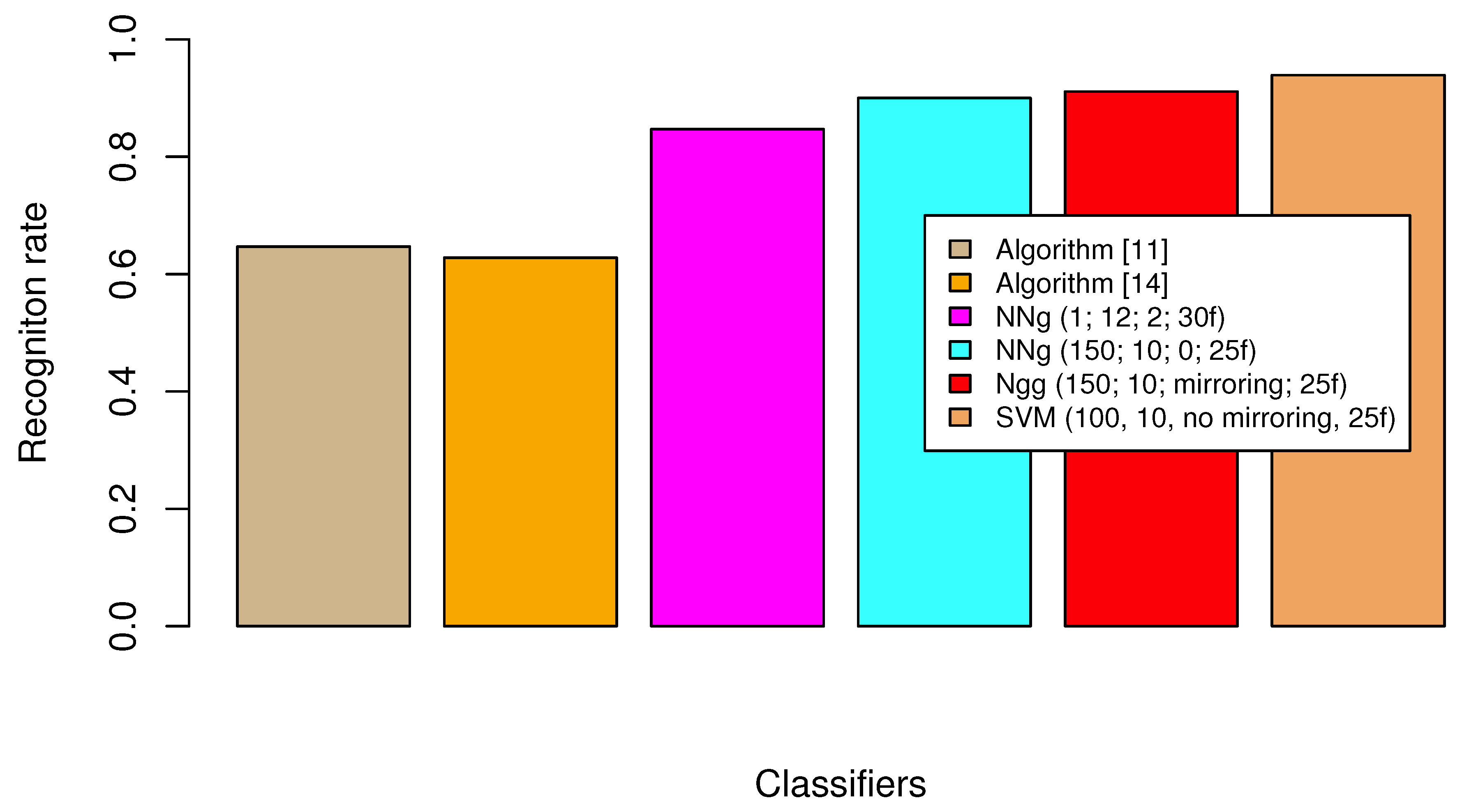
Figure 5 presents a bar chart that compares the recognition rates of the selected classifiers. These classifiers are the algorithm from [11] (tan color); the algorithm from [14] (orange); NNg with a single classifier trained on 12 classes, #augmentation $=2$, with 30 PCA features (this setting has the highest recognition rate in Table 1; magenta); NNg with 150 bagged classifiers trained on 10 classes each, #augmentation $=0$, with 25 PCA features (this setting has the highest recognition rate in Table 2; cyan); SVM with 150 bagged classifiers trained on 10 classes each, mirroring, with 25 PCA features (this setting has the highest recognition rate in Table 3; red); and SVM with 100 bagged classifiers trained on 10 classes each, no mirroring, with 25 PCA features (this setting has the highest recognition rate in Table 4; sandy brown).

4. Discussion

The method presented in [11] uses a two-stage PCA in order to omit the process of MoCap resampling. The initial projection of MoCap data onto 2D space decreases the complexity of the problem and allows for the direct calculation of PCA features. Unfortunately, the evaluation results suggest that this approach simplifies the data too much and that the projected features are not sufficient to correctly classify the whole dataset. Thus, more PCA-based features are required to solve the problem, and it seems that it is better to perform resampling of the original data than to initially minimize the data dimensionality extensively. As shown in Section 3, the algorithm proposed in [14] that utilizes body joint trajectories had far worse results than the method introduced in this paper. This is because spatial trajectory-based coordinates of motions are very sensitive to the differences in motion performance that occur in the top levels of the kinematic chain. For example, the height of a kick (vertical feet position during the kick motion) is mostly determined by thigh mobility. The vertical rotation of the thigh joint affects the vertical position of joints that are lower in the joint hierarchy (leg and foot); however, knee flexions are nearly identical irrespective of the height of the kick. The same condition is true for all spheroid joints. For this reason, spatial body joint positions might not be suitable features for the motion classification task. It is worth mentioning that both methods discussed above had a recognition rate of over 0.62, which is not a bad result for such a difficult dataset.

As shown in the previous section, applying bagging to the classification process improved the recognition rate of both “weak” NNg and SVM classifiers. Using multiple “weak classifiers” that vote on the final classification results led to higher RRs than the RRs resulting from the use of a single classifier of a certain type. For NNg, this improvement was 0.053 (over 5%), while for SVM, the improvement was 0.033 (over 3%). This is a satisfying result, especially for as challenging a dataset as karate MoCap data, in which differences, especially between kicks, are sometimes barely visible. We also have to account for the human factor because the same person might perform an action with varying precision and quality. The application of mirroring (symmetry) with bagging to the NNg classifier improved the RR, while simple augmentation did not have a positive influence on the results. For SVM with a linear kernel, bagging without mirroring resulted in the best RR, while SVM with a radial kernel, bagging, and mirroring produced an RR of 0.922, which is 0.017 worse than the best result. It seems that the obtained recognition rate of $0.94$ might be the limit for this type of feature model on the given tested dataset.

5. Conclusions

The conducted experiment proved that applying the proposed classifier bagging procedure increased the recognition rate of the NNg and SVM classifiers. The RR of the trained classifier (SVM) was higher when we did not use symmetry. On the other hand, when a classifier without optimized decision borders (NNg) was used, symmetry improved its performance. Thus, we can conclude that symmetry information might be helpful for situations in which optimizing the decision borders of the classifier is not possible (for example, when we do not have direct information about class labels). The experiment showed that, in this case, bagging and mirroring might help find a similar object in the training set.

The proposed feature set covers a wide range of motion classes. It uses nearly all tracked body joints. While dealing with a specific motion classification problem other than the one evaluated in this paper, additional tuning of the proposed classifier might be required, similar to that presented in Table 1, Table 2, Table 3 and Table 4, because the final recognition rate might depend on the bagging settings. This adjustment can be easily made with the aid of the source code that is added to this paper. R-language implementation tested various configurations of the proposed solution and showed the results in the form of multiclass confusion matrices.

In sum, it is recommended that the proposed classifier bagging with PCA-based features be applied to MoCap data classification. Moreover, depending on the circumstances, the use of symmetry information in the dataset during the training procedure might improve the results.