3.1.1. Generalized Fibonacci Sequence
The generalized Fibonacci quasi-periodic sequence is given by substitution rule
The corresponding substitution matrix
M is given by
where the elements of the substitution matrix indicate the number of times a given letter,
A or
B, appears in the substitution rule, without considering the order in which these letters occur. The number of letters that appear after applying the substitution rule
j times, is given by the generalized Fibonacci numbers
namely
with
When the number of iterations
j goes to infinity, the ratio between two consecutive Fibonacci numbers
and
tends to a constant number
called the mean of incommensurability, i.e.,
In addition, the relative frequency of both types of letters
and
in the limit
is given by
and
Please note that the mean of incommensurability
can also be obtained as the maximal eigenvalue
of the substitution matrix
M (
55). For the case
and
we obtain the golden mean
, and the corresponding Fibonacci sequence is the following:
Some of the other Fibonacci means [
71,
73,
74] which have been studied are: the Silver mean
the Copper mean
the Bronze mean
the Nickel mean
etc. See Maciá [
73] for a spectral classification of one-dimensional binary aperiodic crystals, studying the eigenvalues
and the determinant
of the substitution matrix
M.
The Fibonacci tight-binding quantum disordered systems have been studied exhaustively by [
37,
38,
40,
41,
42,
43,
44,
45,
46,
59,
60,
63,
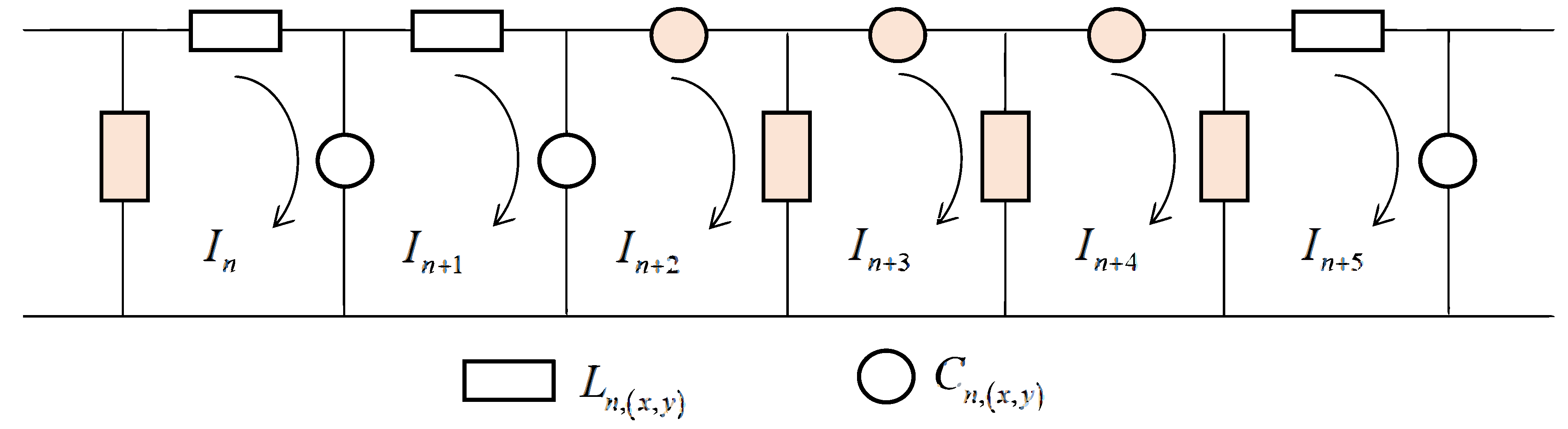
71]. For the diagonal disordered case, the global number of sub-bands is exactly four. However, in the off-diagonal disordered case, the global number of sub-bands is exactly three. In both cases, each sub-band is divided into three sub-bands until it is resolvable. This self-replication behavior is characteristic of quasi-periodic systems. On the other hand, in classical electric systems, dual and mixed transmission lines have been studied [
78,
87] using a Fibonacci distribution of two different values of inductances
and
, namely
Notice that when we introduce disorder in the inductances of the dual or mixed TL, the generic Equation (
3) shows that the disorder appears simultaneously in the diagonal and non-diagonal part.
In dual transmission lines, the localization behavior of the Fibonacci quasi-periodic distribution of inductances
, keeping constant the capacitances
, has been studied [
78] analyzing the spectrum of the generalized Rényi entropies
versus
and the spectrum of the inverse participation ratio
versus
. For each
q value,
and
show more than four global sub-bands. This happens because the allowed frequency band of the dual transmission lines is unbounded from above, namely every frequency of the spectrum is greater than a critical frequency
, i.e.,
At the same time, the spectrum of
and
clearly shows the self-replication behavior, where each sub-band is divided into three sub-bands until it is resolvable (see Figures 2 and 3 of Ref. [
78]). This localization behavior is characteristic of quasi-periodic Fibonacci systems. Inside each sub-band, we find extended and localized states and gaps. When system size
N grows, the number of gaps and localized states increases in such a way that the integrated density of states
behaves in a fractal way. As a consequence, the total bandwidth goes to zero in the thermodynamic limit
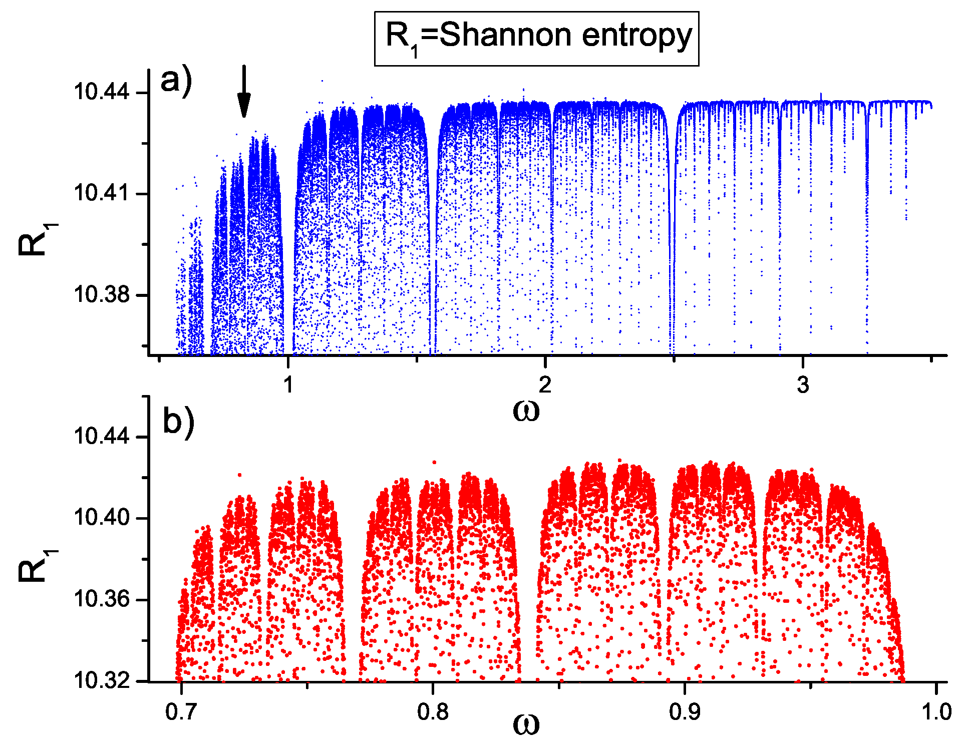
In
Figure 3a) we show the Shannon entropy
(
39), which corresponds to the
Rényi entropy discussed in Ref. [
78]. Notice that the number of global sub-bands is greater than four.
Figure 3b) shows the three sub-bands existing in the global sub-band indicated by the vertical arrow in
Figure 3a). These previous results about the number of global sub-bands of the dual TL shown in Ref. [
78] change when the Fibonacci disorder is introduced in the mixed transmission line [
87]. However, the self-replication of the spectrum is maintained for all kinds of mixed TL formed by
p direct cells and
q dual cells.
Remember that mixed TL are generated by a repetition pattern formed by a group of successive
p direct cells, followed by a group of successive
q dual cells. This topology generates a spectrum of allowed frequencies formed by exactly
bands, as indicated in
Section 2.4. In Ref. [
87], only the
q inductances of the dual cells of mixed TL were distributed according to the Fibonacci sequence, keeping constant the values of the other capacitances and inductances. The localization behavior of the average overlap amplitude
versus
for the case
and
shows three (
) allowed bands (see Figure 10 of Ref. [
87]). These
d bands exist regardless of the type of disorder and the degree of correlation; however, the position of these
d bands depends on the values of all capacitances (
) and inductances (
) of direct cells (labeled
x) and dual cells (labeled
y), and the values of
p and
The average overlap amplitude
versus
shows four global sub-bands, where each sub-band is divided into three sub-bands until it is resolvable (see Figure 11 of Ref. [
87]). This result coincides with the one obtained from the quantum tight-binding model with diagonal Fibonacci disorder. This coincidence occurs because both models (mixed TL and tight-binding model) have bounded spectra and because in both models the Fibonacci disorder appears in the diagonal part of the corresponding dynamic equations (Equations (
3) and (
5)). Conversely, this result is different from the case of the dual transmission line shown in Figures 2 and 3 of Ref. [
78], where the number of global sub-bands is greater than four, because the frequency spectrum of the dual TL is unbounded from the above. Interestingly, when
p and
q change, each of the
bands of the mixed TL can accommodate a different number of global sub-bands. However, the self-replication is always present. To observe this behavior, let us consider the case with fixed
and two different values of
namely
Figure 4 shows the average overlap amplitude
versus
, for (a)
(
bands) and (b)
(
bands). There we can see that the full spectrum of frequencies of mixed TL is contained only within the
d bands.
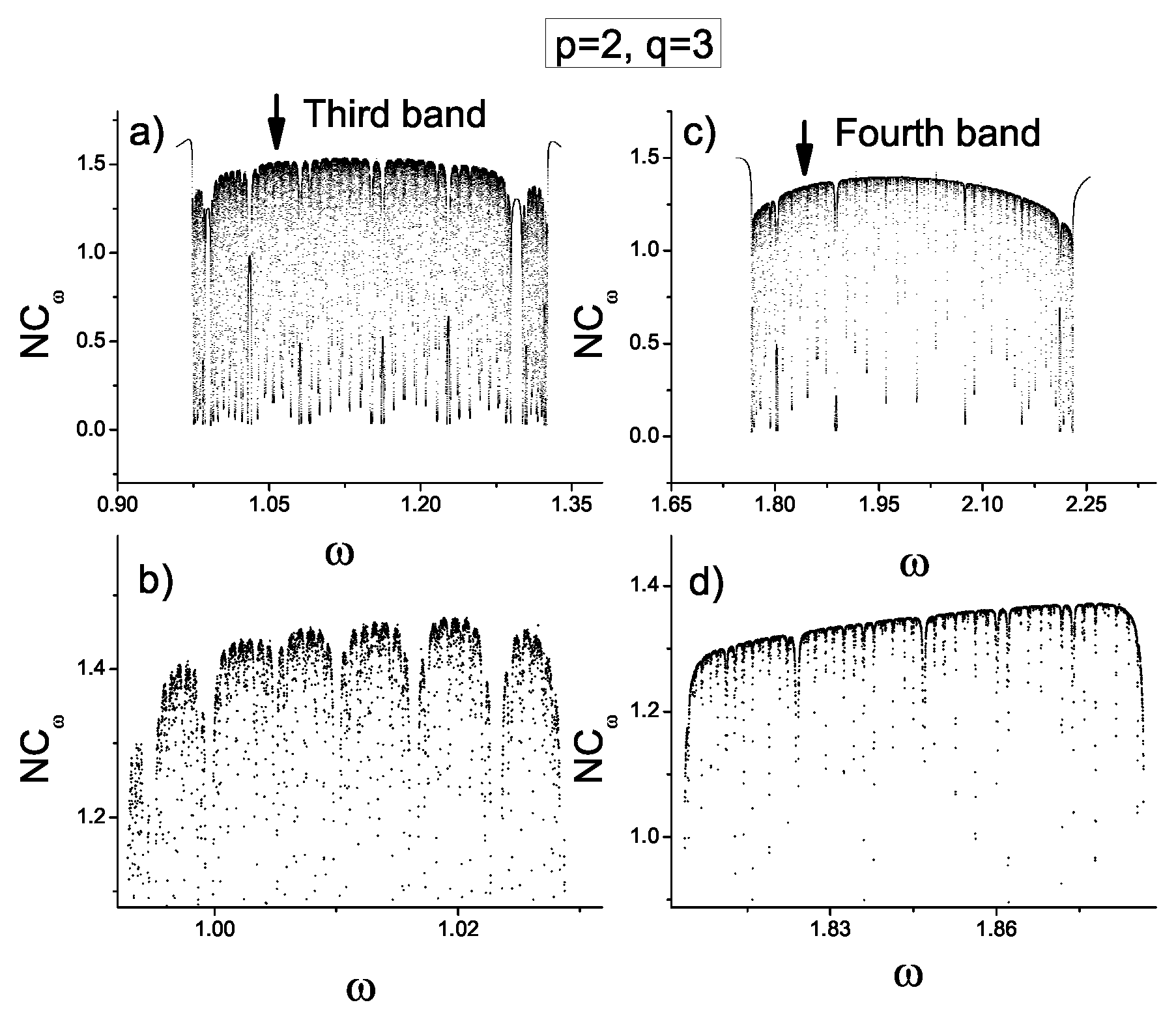
Figure 5 shows
versus
for the third band and fourth bands shown in
Figure 4b. In addition,
Figure 5b,d show the self-replication behavior of each sub-band indicated with a vertical arrow in
Figure 5a,c, respectively. In this figure we can see that the number of localized states and gaps increases after each self-replication.
In summary, for arbitrary values of p and q forming the mixed TL, the set of bands accommodates the full spectrum generated by the Fibonacci distribution of inductances Inside each of the d bands, the number of global sub-bands is always greater than or equal to four, and the self-replication behavior corresponding to quasi-periodic systems is always present. In the self-replication process, new localized states and gaps appear repeatedly. Consequently, the integrated density of states has a fractal behavior and in the thermodynamic limit.
3.1.2. Generalized Thue–Morse Sequence
The generalized Thue–Morse (TM) aperiodic sequence can be generated by means of the substitution rule
The corresponding substitution
M matrix is given by
The
maximal eigenvalue of
M is
For the case
and
we obtain the usual Thue–Morse sequence:
namely
The maximal eigenvalue
is thus the length of the substitution, which means that
is the number of the
A and
B letters in the
kth iteration. For the generalized Thue–Morse sequence, the relative frequency of both types of letters,
and
, is the following
and
Another generalization of the Thue–Morse sequence is the
tupling sequence generated by the substitution rule
with
In this case, the maximal eigenvalue of the corresponding substitution
M matrix is
and the number of letters
N in this sequence also increases geometrically, i.e.,
where
k is the iteration order. Here
For
we return to the usual Thue–Morse sequence. A spectral classification of one-dimensional binary aperiodic crystals as a function of the substitution matrix
M is shown in Ref. [
73].
For the tight-binding quantum model, the aperiodic properties of the generalized Thue–Morse systems have been studied in great detail by [
47,
48,
49,
50,
51,
52,
53,
54,
55,
56,
57,
58,
60,
62,
71]. Additionally, in classical dual and direct transmission lines the Thue–Morse and the
tupling distribution of capacitances and inductances have been studied by [
83,
84,
85]. For direct TL, two values of inductances
and
where distributed according to the
tupling substitution rule
keeping constant the capacitances [
83,
84]. For
we obtain the usual Thue–Morse substitution rule
One of the principal findings of these studies was that the localization properties of the usual Thue–Morse case, namely
is markedly different to the
case. In general, although in the
tupling sequence the number of letters
A and
B in each iteration is the same (
) for any value of
the number of extended states in the
tupling inductance distribution depends on the specific value of
This was demonstrated numerically using different localization tools, like normalized localization length
participation number
normalized participation number
global density of states
transmission coefficient
and the average overlap amplitude
In addition, it was shown that inside the
tupling family, starting with
the number of extended states increases as the value of
m increases, so that for
, the allowed spectrum is similar to the spectrum of the case
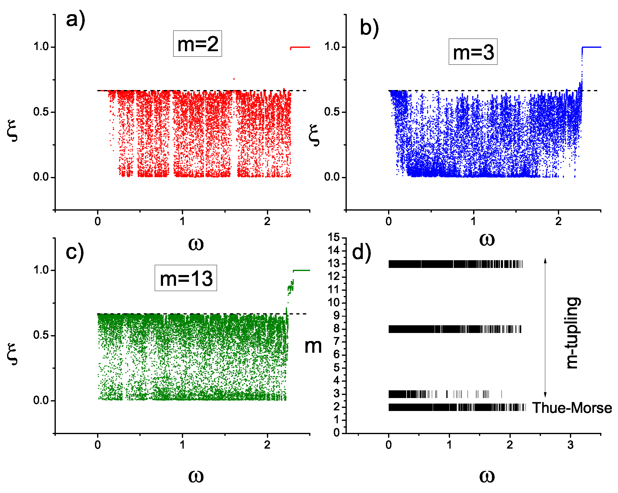
(Thue–Morse). This can be seen in
Figure 6 where we show the normalized participation number
for three values of
namely
(a) to (c). Also, in
Figure 6d we indicate with a short vertical bar the spectrum of the extended states, namely the frequencies for which the
normalized localization length meets the condition
. The image shows that the number of extended states for
is small compared to the case
. However, for the case
, namely
and
the number of extended states becomes comparable with case
.
When comparing the spectrum for cases
and
in a restricted region of frequencies (see
Figure 7), it can be observed that the number of extended states which fulfills the condition
, corresponding to the periodic case, is reasonably similar in both cases. Also, we can see that the sub-band of extended states of the Thue–Morse case with
(
Figure 7a) is much wider than the sub-bands of extended states of the
tupling case with
(
Figure 7b).
In sum, for direct transmission lines with
tupling distribution of inductances, the frequency spectrum of the Thue–Morse sequence (
) can be considered the limit of the
tupling sequence’s frequency spectrum when
On the other hand, the number of extended states for the case
decreases dramatically when
m changes to
as shown in Refs. [
83,
84] and
Figure 6.
As an extension of these ideas, the localization behavior of dual transmission lines with non-linear capacitances has been studied [
85]. The non-linear behavior of capacitances is introduced through the
potential difference across each capacitance, i.e.,
is the linear part of the capacitance
and
is the amplitude of the non-linear term. The equation corresponding to this dual case is given by
When the non-linear amplitudes
go to zero (
), we return to the dual linear Equation (
2). The localization behavior of this non-linear dual TL has been studied using two values of the non-linear amplitude
namely
and
, distributed according to the
tupling Thue–Morse sequence [
85], i.e.,
, but keeping constant the capacitances
and inductances
, namely
and
In this case, the aperiodic disorder appears only in the diagonal term of the dynamic Equation (
59).
The same fundamental result about the localization degree of the
case in comparison with the
case reappears in this non-linear case, that is, for fixed values of
and
the
family does not belong to the family corresponding to
and in addition, for
the frequency spectrum begins to resemble the spectrum of the case
To be specific, for
we can see a large number of extended states across the entire frequency spectrum, mixed with localized states and gaps. On the contrary, for
almost the entire frequency spectrum is formed with localized states and gaps, accordingly showing a huge decrease in the number of extended states. This behavior can be seen in Figure 6 of Ref. [
85] that shows
versus
for
. To compare the cases for
and
in more detail, in
Figure 8 we show the average overlap amplitude
, for
with
and
keeping constant the values of capacitances
and inductances
. When
m changes from
to
the number of extended states decreases markedly, almost tending to zero. The horizontal dashed line corresponds to the periodic linear case,
for which
fulfills the condition
. Moreover, at the top of each figure, we indicate with a short vertical bar the presence of an extended state, namely
. Both results about the number and position of the extended states in each case match each other. This localization behavior coincides with the results shown in Figure 6 of Ref. [
85], when studying the localization behavior of the normalized participation number
and
This way, we have demonstrated that the
(Thue–Morse) case is different than the
case (
tupling).
Consider now the localization behavior of the integrated density of states
for the non-linear case, with
and
. In
Figure 9a we show the
for four values of
namely
. For each
m we use a constant size
namely
There we can see that for the case
the
is always greater than the
of any other value of
However, when
m grows (
and
), the
grows, approaching the values for the case
This behavior confirms the conjecture that the Thue–Morse sequence (
) can be considered to be a limit case of the
tupling sequence when
We now turn to the behavior of the
for fixed
as a function of the
system size, with
(see
Figure 9b). For the minimum value
, the
is the greatest of all, but when
N increases (the value of
k increases), the number of extended states decreases (the
decreases), and new localized states and gaps appear that barely contribute to the integrated density of states. As a consequence, the
tends to zero. This behavior is characteristic of aperiodic systems.
On the other hand, for fixed value of
m, when the difference
between the values of the amplitudes of the non-linear term increases, so does the disorder degree of the transmission line, which tends to localize the electric current function
and as a result, the integrated density of states
go to zero. This behavior can be observed in Figure 5 of Ref. [
85], for
(Thue–Morse case), considering a fixed value
(the periodic linear case) and three different values of
, namely
3.1.3. Incommensurate Sequences
The aperiodic incommensurate systems are generated by two superimposed periodic structures with incommensurate periods. The origin of incommensurability may be structural or dynamic. In the first case, two or more superimposed periodic structures with incommensurate periods exist, and in the second case one periodicity is related to the crystalline structure and the other to the behavior of elementary excitations that propagate through the crystal. Two of the most studied incommensurate models are the Aubry–André model and the Soukoulis–Economou model.
In the one-dimensional tight-binding quantum model, the site energies
have been distributed according to the Aubry–André model that is
where
is the single-site energy of the unperturbed periodic lattice,
b is the amplitude and
is an irrational number, usually
(the inverse of the Fibonacci golden mean). For
, a phase transition from extended to localized states appears [
36,
69,
70,
72].
In classical electric transmission lines, the Aubry–André model has been used to distribute the inductances
in two different cases: (a) direct TL with constant capacitances
(diagonal disorder) [
86] and (b) mixed transmission lines with disorder only in the
q inductances of the dual cells, keeping constant the value of all the other electrical components of the direct and dual cells [
87]. In this case, the disorder appears in the diagonal and the off-diagonal terms of the generic Equation (
3).
In case a), the inductances
of the direct transmission line are distributed according to the Aubry–André sequence:
where
and
. In this case, the aperiodic incommensurate disorder only appears in the diagonal term of the generic Equation (
3). The localization behavior of this classic electric model can be visualized in
Figure 10 where the map
is shown for
and
. Each dot on the map indicates the existence of an extended state, because the normalized localization length fulfills condition
For
, the frequency spectrum shows a single band of extended states that corresponds to the periodic case. For increasing values of
b, i.e., for
, the map
shows three global sub-bands of extended states (with localized states and gaps) separated by two large gaps. After that, for
, only two global sub-bands of extended states survive, which also contain localized states and gaps. Finally, for
b close to
there is only a small sub-band where almost all states are extended states, namely
.
Figure 11 shows (a) the
Lyapunov exponent versus
for two values of the
b amplitude
and b the spectrum of the extended states,
versus
for fixed
Figure 11a shows that for
(thick red line), only one band of extended states (
) can be observed for
Conversely, for
only gaps and localized states can be found for this value of
This result coincides with the result indicated by the map shown in
Figure 10. On the other hand, in the same
Figure 11a we draw
versus
for a smaller value of
namely
(thin black line). There we can see several sub-bands of extended states (
) separated by gaps. Within these sub-bands, we can find more localized states and gaps, which are not perceived in this picture. On the contrary, these gaps can be seen in
Figure 11b, where a detail of the map
Figure 10 is shown for
for fixed
In this figure, each short vertical bar indicates an extended state, because
The vertical dashed arrows that cross both figures (for the case
) indicate the edge of the gaps, i.e., the frequencies for which phase transitions occur.
To see in more detail the phase transition from extended to localized states, in
Figure 12a we show the Lyapunov exponent
versus
for the cases
and
The vertical arrows indicate the frequencies
and
to be studied in
Figure 12b–d, respectively. In these last three images, we show the scaling behavior of the average overlap amplitude
for three values of
namely
For each frequency
and
we find a phase transition from extended states to localized states at the critical value
To the left of the critical point
for almost every amplitude
b, all
values coalesce into a single one, i.e.,
indicating an extended behavior. On the contrary, to the right of the critical point (
),
grows as system size
N grows, indicating a localized behavior.
These results coincide with those in Figures 4–6 of Ref. [
86], where this same problem was studied. In [
86], a phase transition from the extended to the localized state is found depending on amplitude parameter
b. This result was found for different frequency values, by studying transmission coefficient
and the scaling behavior of the average overlap amplitude
.
In case (b), for mixed transmission lines (with
p direct cells and
q dual cells), the inductances
of the
q dual cells were distributed according to the Aubry–André sequence [
87], namely
with
. All other electric components are kept constant, i.e., for direct cells
and for dual cells
. In Ref. [
87], three different cases were studied: (a)
, (b)
and (c)
In all cases, the frequency spectrum is completely contained within the
bands generated by the mixed TL. For fixed
b, in each of the
d bands, it is always possible to find sub-bands of extended states in addition to localized states and gaps. These results were obtained by studying the transmission coefficient
and the scaling of the average overlap amplitude
(see Figures 7–9 of Ref. [
87]). To see the influence of the
b amplitude in the localization behavior, in
Figure 13 we show the transmission coefficient
for four values of
b, namely
for the case
We use the same values of the electric components used in Ref. [
87]. In particular,
For
we find
bands containing extended states, localized states and gaps (similar to Figure 7a of Ref. [
87]). However, for increasing values of
the number of extended states within each band decreases, and as a consequence both lateral bands begin to disappear. In this way, for
, the leftmost band has already disappeared, and for
the rightmost band is about to disappear.
3.2. Long-Range Correlated Disorder
For one-dimensional disordered systems without any correlation in the disorder (white noise), all states are localized states in the thermodynamic limit. However, the introduction of correlation in the disorder can trigger the appearance of a discrete set of extended states (short-range correlation) or bands of extended states (long-range correlation). The correlated disorder has been introduced in quantum tight-binding systems [
2,
3,
4,
5,
6,
7,
8,
9,
10,
11,
12,
13,
14,
15,
16,
17,
18,
19,
20,
21,
22,
23,
24,
25,
26,
27,
28,
29] and in classical systems such as harmonic chains [
96,
97,
98,
99], and electrical transmission lines [
76,
77,
79,
80,
88].
The quantum tight-binding Equation (
5) and the generic Equation (
3) describing transmission lines are similar. Transformations (
6) and (
7) permit the correspondence between both models. However, unlike the quantum case, in transmission lines it is impossible to study the pure off-diagonal case, because the disorder contained in the vertical impedances (the coupling between neighboring electric cells) appears in the off-diagonal coefficients
and
of the generic Equation (
3) and in the diagonal coefficient
too.
To analyze the main differences in the localization behavior with the one-dimensional quantum case, the dual, direct and mixed disordered transmission lines have been studied recently. These studies include long-range correlated disorder and diluted disordered TL. In addition to continuous sequences, the long-range correlation has been used to generate discrete sequences (binary and ternary).
3.2.1. Discrete Sequences
To generate long-range correlated sequences we use the Fourier filtering method (FFM). Let us consider initially a set of uncorrelated random numbers with a Gaussian distribution. Then we take the fast Fourier transform (FFT) of the random sequence and we obtain a new sequence The long-range correlation is introduced in the sequence doing the following transformation Calculating the inverse FFT of the new sequence we obtain the long-range correlated sequence which is spatially correlated with the spectral density Here the exponent of the transformation is known as the correlation exponent and fulfills the condition . For we regain the uncorrelated random sequence (white noise). Correlation exponent quantifies the degree of long-range correlation imposed in the original random sequence . Finally, we normalize the correlated sequence to obtain zero average, and the variance is set to unity.
From the long-range correlated sequence
we can generate the asymmetric ternary sequence
formed with three letters,
B and
with
The symmetric ternary map is obtained when
If
we obtain the asymmetric binary sequence
. For
we regain the symmetric binary sequence. Please note that the long-range correlation of the ternary sequence
is not exactly quantified by the correlation exponent
because the map (62) changes the long-range correlation. In one-dimensional tight-binding systems, the symmetric binary and ternary model has been studied [
8,
24,
25,
28]. In these models, a metal-insulator transition has been reported as a function of the correlation degree
and size
b of the window. In addition, the asymmetric ternary map (62) was studied using electrical dual transmission lines [
76] considering three values of capacitances
maintaining constant the inductances
This case contains only diagonal disorder. The long-range correlation in the distribution of capacitances was generated through the FFM. For TL with a finite number of cells, it is possible to find bands of extended states whose size increases for increasing values of correlation exponent
. For the asymmetrical model, the normalized localization length
is a complicated function of the parameters
and
N, but for fixed frequency
for
it is always possible to find a transition from localized electric current functions to extended current functions for some specific values of the parameters. For the symmetrical ternary map
, a phase diagram
separating localized states from extended states has been found for fixed frequency performing finite-size scaling of the normalized localization length
This result is similar to the phase diagram found in the tight-binding case.
Moreover, the same ternary dual TL was studied, but using the Ornstein–Uhlenbeck method to generate the long-range correlation [
77]. In this method, the degree of long-range correlation depends on two independent parameters, i.e., the viscosity coefficient
and the diffusion coefficient
Studying the scaling behavior of
we obtain two-phase diagrams for the symmetrical map when
C and
are independent parameters, namely
for fixed
and
for fixed
In addition, we study the phase diagrams when
C and
are dependent parameters, i.e.,
. In all cases, we find a transition from localized to extended states. Also, the harmonic symmetric ternary chain was studied in Ref. [
99] using the Ornstein–Uhlenbeck method for the case
Instead of the transition from localized to extended behavior, they found a disorder-order transition for
because the disorder degree practically disappears at this limit.
This same kind of disorder-order transition has been found by studying localization properties of direct TL with diluted and non-diluted asymmetric dichotomous noise (binary sequences of inductances
and
with
) [
82]. The asymmetric dichotomous sequence
is generated by a variable
which switches in time in a random way between two given values
a and
with transition rates
and
respectively (dichotomous noise). Considering
as a stationary process, the dichotomous noise has zero mean and is exponentially correlated. The
correlation time of the dichotomous noise is defined as
In addition, from the zero-average condition
we obtain the following relationship between
and
namely
where parameter
measures the degree of asymmetry of the dichotomous noise. For
we have
and for
we have
The symmetric sequence
is obtained for the case
. Consequently, the dichotomous noise is characterized by three independent parameters:
a and
However, setting the value of one of the parameters, for example,
we can study the localization behavior generated by this kind of exponentially correlated noise using only two independent parameters, i.e.,
and
. In the diagonal disordered direct TL, the inductances
and
are distributed according to the asymmetric dichotomous noise, keeping the capacitances constant
[
82]. For
and for
(
are critical values) the electric current function
shows a localized behavior, but for
and for
the
participation number scales as
where
is the slope of the linear relationship between
and
for fixed
, and
Only in the limit
(for fixed
and
) and
(for fixed
and
), we obtain the exact linear behavior, i.e.,
and
However, in both limits,
or
the asymmetric dichotomous sequence becomes a periodic sequence. Thus, we only can observe a disorder-order transition, which in turn indicates that all states are localized states in the thermodynamic limit for classical electric TL. This result coincides with the one obtained for the one-dimensional tight-binding quantum model with symmetric dichotomous noise, in which the metal-insulator transition is absent [
56,
100].
3.2.2. Continuous Sequences
In addition to discrete sequences, continuous long-range correlated sequences have been used to study the localization behavior of direct, dual and even mixed electrical transmission lines [
79,
80,
88]. In general, in classical electric transmission lines, the long-range correlated disorder in capacitances and inductances has been used in the following form:
and
where
is an harmonic function.
and
are two independent long-range correlated sequences generated by the FFM and
and
are the corresponding correlation exponents that determine the correlation degree.
b is the amplitude of the fluctuation of
and
around
and
respectively. The diagonal and off-diagonal disordered dual transmission line, considering only one type of correlated sequence
has been studied recently [
79]. In this case,
and
vary in phase, i.e.,
Here, to avoid negative values of the electrical components. For this kind of disorder, it is always possible to find extended states for different frequencies, and for each specific frequency a phase diagram , which separates extended states from localized states in the thermodynamic limit can be found.
To obtain the critical correlation exponent
separating localized states from extended states, we analyze the scaling behavior of (a) the participation number
(
37), (b) the relative fluctuation
of the participation number
and (c) the Binder cumulant
of the participation number
These quantities are defined as
and
where
means an average over long-range correlated sequences.
For increasing system size
N, the relative fluctuation
goes to zero for extended states and grows converging to a finite value for localized states. Consequently, for
tends toward a step function and a discontinuity appears that separates extended states from localized states. This scaling behavior can be used to determine the critical correlation exponent
for fixed values of
and
because the curves
with different
N values will cross in a single point (the critical point
). Also, the scaling behavior of the Binder cumulant
indicates that for
jumps abruptly from a constant value (
) for extended states to zero (
) for localized states. Consequently, for fixed values of
and
the curves
with different
N values will cross in a single point (critical point
). On the other hand, the critical value of the fluctuation amplitude
can be obtained studying the scaling behavior of the normalized localization length
(
35). For fixed
and
, in the transition point from localized to extended states,
varies from
to
Finally, in the thermodynamic limit, for fixed frequency
the phase diagram
is formed by two independent straight lines, so that extended states only appear when condition
is met for any
. Specifically, in Ref. [
79] the following values were used:
. For the fixed frequency
the critical values are
and
(see phase diagram in Figure 9 of Ref. [
79]). In
Figure 14 we show, in a schematic way, the phase diagram for a fixed frequency
, when
and
vary in phase (63) in dual TL. This map is conceptually different to the map in
Figure 15b), when
and
vary out of phase (in the study of mixed TL).
In Ref. [
88], this model was generalized in two ways: (a) studying mixed transmission lines instead of dual TL, and (b) the capacitances
and inductances
of the dual cells of mixed TL are distributed out of phase, using two independent long-range correlated sequences
Specifically,
where
and
are two independent long-range correlated sequences, even in the case
because each correlated sequence is initiated using two independent uncorrelated random sequences according to the FFM. The localization behavior of this mixed TL was studied in Ref. [
88] for the case
. The frequency spectrum of this case shows
bands. Additionally, in the thermodynamic limit, for fixed
p,
q and
b, it is always possible to find an asymmetric phase diagram
for each frequency
corresponding to an extended state. In the case studied in Ref. [
88], for
and
the correlation exponents
and
fulfill the following condition:
and
with the asymmetric condition
. This behavior can be observed in Figures 8 and 9 of Ref. [
88]. There we can see the phase diagram
that separates localized states from extended states, and the localization behavior of
versus
(for fixed
), and
versus
(for fixed
). The asymmetric condition
can be explained through the following arguments. In relationships (66), the fluctuation
of the capacitances around
is the same as the fluctuation of inductances
around
namely
However, in every kind of transmission line, capacitances only appear in the form
Accordingly, the fluctuation of this term is given by
where
For
we have
which means that the term
introduces a greater disorder into the generic Equation (
3) than the disorder introduced by
. This fact can induce a decrease in the degree of correlation of the sequence
To compensate this decrease, correlation exponent
must be greater than correlation exponent
of
to generate extended states. Consequently, the critical correlation exponents fulfill the condition
as long as condition
is valid. Also, for fixed
, and for given correlation exponents
and
it is possible to find a critical value of amplitude
b of the fluctuation, in such a way that for
all states are localized states (see Figures 10 and 11 of Ref. [
88]).
The localization behavior of mixed transmission lines with long-range correlated disorder given by (66) can be summarized in
Figure 15 and
Figure 16, where we studied mixed TL with
and
This case has
bands.
Figure 15a shows
versus
for
for two fixed values of the correlation exponents, namely
and
Only three bands are visible, because
for the leftmost band (localized states). The vertical arrow indicates the specific frequency
studied in
Figure 15b and
Figure 16. For this frequency,
Figure 15b shows the phase diagram
This image indicates that only for
and
, with
it is possible to find extended states. Also, for
the critical correlation exponents are
and
Please note that the asymmetric condition
is fulfilled.
Figure 16 shows the scaling behavior of the average overlap amplitude
versus
for the frequency
indicated by vertical arrows in
Figure 15a. For fixed
we obtain the critical value
of the correlation exponent, namely
(see
Figure 16a). For
all states are localized states because we cannot obtain a linear relationship between
and
. However, for
we only find straight lines with the same slope
(
). This behavior indicates that
is constant for increasing values of
This is exactly the scaling behavior of the average overlap amplitude for extended states. For fixed
,
Figure 16b shows the same kind of scaling behavior, obtaining
3.3. Diluted Disordered Systems
Hilke [
101] introduced the diluted Anderson model, which considers two interpenetrating lattices, i.e., a pure lattice (
), while an Anderson lattice (
is a random number) is periodically distributed with period
This means
diluting elements exist between two Anderson sites. For
we regain the usual Anderson model [
1]. This model was generalized [
11,
12] so that the
diluting elements are distributed according to a function with certain specific symmetry conditions (see Ref. [
11]). The case
is the most symmetrical of all, and coincides with the results from previous works [
101,
102,
103]. Depending on the type of symmetry, the dilution process can generate a maximum of up to
extended states, which are exactly located on some of the edges of the gaps. For constant off-diagonal term, the position of these resonances depends only on the period
P and the values of
of the diluting elements. At the same time, resonances are independent of the type of disorder, as well as the degree of correlation in the disordered lattice. In addition, in the resonance, the extended wave function behaves like an intermediate extended function, because its amplitude is zero at each disordered site. The localization behavior of the diluted systems have been studied in the tight-binding quantum case, and in classic systems, like harmonic chains and electric transmission lines [
11,
12,
15,
23,
80,
81,
82,
84,
96,
101,
102,
103].
Let us consider the localization behavior of diluted direct transmission lines, with constant capacitances, i.e.,
The inductances
corresponding to disordered sites, have been distributed in different forms. Between two disordered inductances,
and
, we put
identical inductances
where
Consequently, the inductances are distributed in the following schematic way ...
..., where
. Because of the full symmetry of the diluting elements, we find exactly
resonances and
gaps [
11]. For direct transmission lines, resonance frequencies are obtained analytically [
80,
81,
82]:
where
and
In Ref. [
80] the inductances
were distributed in (a) a random way, and (b) considering long-range correlated disorder (Fourier Filtering method and Ornstein–Uhlenbeck process). In both cases a continuous distribution of
values was used. In addition, in Ref. [
81] the inductances
were distributed by means of an aperiodic binary sequence of Galois [
67], and in Ref. [
82] the inductances
were distributed considering an asymmetric dichotomous sequence. In all cases studied, the existence of
intermediate extended states has been demonstrated. Also, the position of the resonance frequencies coincides with theoretical predictions.
On the other hand, the localization behavior of the diluted aperiodic
tupling distribution of inductances was studied in Ref. [
84]. The case
was considered, with
diluting elements
. For numerical calculation, the following data were used:
and
Figure 6 of Ref. [
84] shows (a) the overlap amplitude
and (b) the normalized participation number
. In that picture we can see four gaps and four resonances, which are indicated by vertical dashed lines. Notice that resonances are placed at the left edge of each gap. This result coincides with the theoretical predictions. In
Figure 17, we show the average overlap amplitude
for the same case studied in Figure 6 of Ref. [
84], but now we study the Thue–Morse sequence, i.e.,
Here, we consider four values of
namely
The case
corresponds to the usual Thue–Morse sequence without dilution. According to (67), for each
the frequency of the resonances are:
and
These theoretical values coincide with the numerical results shown in
Figure 17. The same localization behavior of this diluted aperiodic system can be seen in
Figure 18 studying the density of states
versus
There we can see that to the left of each gap, the density of states does not fluctuate, which is an indication of the extended nature of the resonance located there. This does not happen on the right side of each gap.
4. Summary and Conclusions
We have presented the results of the study of the localization properties of disordered electrical transmission lines. This study considered three types of TL: dual, direct and mixed. The electrical components of the (capacitances and inductances) were distributed in different non-periodic forms: (a) aperiodic, which included self-similar sequences (Fibonacci and tupling Thue–Morse), (b) incommensurate sequences (Aubry–André and Soukoulis–Economou), and (c) long-range correlated sequences (binary discrete and continuous). The localization properties of these classical systems were measured using the typical tools used in quantum mechanics to characterize the localization behavior of disordered systems. Specifically, we used the normalized localization length , the inverse participation ratio , the transmission coefficient , the global density of states the average overlap amplitude , and others. Our studies indicate that the localization behavior of classic electric transmission lines is quite similar to the one-dimensional tight-binding quantum model, but at the same time it is possible to observe some significant differences; therefore, it is worth continuing to investigate this type of classical disordered systems.
As a possible application of the study of the localization properties of disordered electric transmission lines, we can consider the neuronal axons that connect two or more neurons through electrical impulses. The axon, which usually is covered by a myelin sheath, can be considered to be a transmission line formed by Schwann cells connected by nodes of Ranvier. It has been established that there exist certain specific genes responsible for stabilizing the internal neuronal structure, which in turn allows the proper transport of the electrical impulse within the axon. The electrical communication between neurons fails if axons are damaged or broken. This can happen in the earliest stages of neurodegenerative diseases or for other reasons. Based on the localization properties of electrical transmission lines studied in this review, it is possible to conclude that electrical communication between neurons prevails, if Schwann cells and Ranvier nodes are distributed in a periodic way or in a very specific aperiodic way. On the contrary, any non-correlated disorder in the axon structure will stop the electrical impulses and the neurons will remain without communication. Consequently, to restore electrical communication between neurons, I can conjecture that the genes responsible for stabilizing the internal neuronal structure have the specific mission of restoring periodicity in the distribution of Schwann cells and Ranvier’s nodes.
Up to that point, we have only considered ideal transmission lines, i.e., transmission lines without dissipation (resistance
). When we introduced gain (
n odd) and loss (
n even) balanced pairwise, a
-symmetric resistive configuration is obtained. For this dissipative system, we can find a critical resistance
such that for
the frequency spectrum is completely real, but for
the frequency spectrum contains real and complex frequencies. This phenomenon is called a
-symmetric transition phase, because the TL goes from an unbroken (
) to a broken
-symmetric phase as a function of resistance
R. In addition, we have demonstrated that in the unbroken
-symmetric phase, the electric current function
is a symmetric extended function. Conversely, in the broken phase,
is an antisymmetric localized function. This phase transition was recently found for TL with a very small number of cells considering fixed boundary conditions [
89].
In addition to this research, we are currently studying two different lines of research, (a) the influence of non-linear inductances or capacitances in the stability and amplitude of the allowed conducting bands of the unbroken
-symmetric phase, and (b) the localization behavior of some models of structured transmission lines, in the spirit of the structured systems proposed by Chakrabarti [
29]. Specifically, we analyzed TL with a finite number of hanging cells (direct or dual) in random positions in TL. The electric components (capacitances or inductances) of each hanging cell, can contain aperiodic disorder or long-range correlated disorder.


