Article

Approximate Multi-Degree Reduction of SG-Bézier Curves Using the Grey Wolf Optimizer Algorithm

1
Department of Applied Mathematics, Xi’an University of Technology, Xi’an 710054, China
2
Department of Mathematics & Computer Science, University of North Carolina at Pembroke, Pembroke, NC 28372, USA
*
Author to whom correspondence should be addressed.
Symmetry 2019, 11(10), 1242; https://doi.org/10.3390/sym11101242
Submission received: 26 July 2019 / Revised: 21 September 2019 / Accepted: 25 September 2019 / Published: 4 October 2019

Abstract

:
SG-Bézier curves have become a useful tool for shape design and geometric representation in computer aided design (CAD), owed to their good geometric properties, e.g., symmetry and convex hull property. Aiming at the problem of approximate degree reduction of SG-Bézier curves, a method is proposed to reduce the n-th SG-Bézier curves to m-th (m < n) SG-Bézier curves. Starting from the idea of grey wolf optimizer (GWO) and combining the geometric properties of SG-Bézier curves, this method converts the problem of multi-degree reduction of SG-Bézier curves into solving an optimization problem. By choosing the fitness function, the approximate multi-degree reduction of SG-Bézier curves with adjustable shape parameters is realized under unrestricted and corner interpolation constraints. At the same time, some concrete examples of degree reduction and its errors are given. The results show that this method not only achieves good degree reduction effect, but is also easy to implement and has high accuracy.

1. Introduction

Parametric curves are not only an important research deimension in the fields of CAD/CAM, but they also play a crucial role in the shape design and geometric representation of various products. The simple, intuitive structure and many excellent properties of the traditional Bézier curve means that it has become one of the important methods of representing curves in CAD/CAM systems. However, the shape of Bézier curves is uniquely determined by the control points, which is not convenient for engineering application and design. In response to this shortcoming, the scholars proposed rational Bézier curves by introducing a weight factor, adjusting or modifying the shape of the curves without changing the control points. However, the introduction to rational fractions will lead to many problems, such as computational complexity, inconvenient integration, repeated derivation, and so on [1,2].
To maintain the advantages of the Bézier method and increase the ability to adjust its shape, as well as to improve its approximation to real curves, scholars have constructed many non-rational Bézier curves with shape parameters [3,4,5,6,7,8,9,10,11,12,13,14,15,16,17,18,19]. Based on a new set of generalized Bernstein basis functions of explicit expressions, Hu et al. [20] proposed a generalized Bézier (SG-Bézier) curve with various shape parameters. This curve not only inherits many excellent characteristics of Bézier curves, but also has flexible shape adjustability. It can adjust the shape of the curves by changing the global and local shape parameters to construct more complex curves with degrees of freedom. According to the basis functions and endpoint property of SG-Bézier curves, Hu and Bo gave the continuity conditions of G1 and G2 between two adjacent SG-Bézier curves, and studied the smooth joining steps of SG-Bézier curves and the influence of shape parameters on complex curves [21]. At present, there is no report on the degree reduction of SG-Bézier curves.
Based on the different requirements for the degree of curves in different CAD/CAM systems, the degree reduction of the curves can better realize the data conversion and transmission between different systems. There are three main types methods of degree reduction of curves: one is based on the geometric properties of the control points. Some scholars use the geometric properties of the curves itself and combine the generalized inverse matrix and the least square theory to achieve the degree reduction of the curves [22,23,24]. Based on the least squares rule, Gospodarczyk [25] achieved the degree reduction of Bézier curves by strengthening the constraints of the control points region. One kind of algebraic method is based on basis transformation. Ahn [26] proposed an approximate degree reduction algorithm based on constrained Jacobi polynomial that maintains the curves reach Ck,k continuity at the endpoints. Lee et al. [27] gave a multi-degree reduction algorithm by using the transformation between Bernstein basis and Legendre basis. In 2006, Rabah et al. [28] gave a multi-degree reduction algorithm for Bézier curves with endpoints constraints by using the transformation matrix between Bernstein basis and Chebyshev basis and the elevation matrix of Chebyshev polynomial. One method is to transform the problem of degree reduction into solving the optimization of objective function by using intelligent optimization algorithm; Ahn et al. [29] showed that the constrained polynomial degree reduction in the L2-norm equals best weighted Euclidean approximation of Bézier coefficients. In 2016, Ait-Haddou and Bartoň [30] illustrated that a weighted least squares approximation of Bézier coefficients with factored Hahn weights provides the best constrained polynomial degree reduction with respect to the Jacobi L2-norm. Lu and Qin [31] proposed a method for the degree reduction of S-λ curves using a GSA algorithm. Based on the theory of grey wolf optimizer (GWO) algorithm [32,33,34,35], this paper considers the degree reduction of SG-Bézier curves under unrestricted condition and constraint condition of C0 and C1. The numerical examples show that the algorithm can find the global optimal SG-Bézier curve more quickly and accurately.
The remainder of this paper is as follows. The SG-Bézier curves and GWO algorithm are described in Section 2 and Section 3, respectively. In Section 4, we propose the multi-degree reduction of SG-Bézier curves using GWO algorithm. Some applications are given in Section 5. Finally, a brief conclusion is given in Section 6.

2. The Definition of SG-Bézier Curves

Let B j , n ( t ) = ( n j ) ( 1 t ) n j t j , t [ 0 , 1 ] is the jth Bernstein basis function of degree n, and [ n 2 ] = [ n / 2 ] = { n / 2 , if   n   is   even ( n 1 ) / 2 , if   n   is   odd .
Definition 1.
For any t [ 0 , 1 ] , n 2 , n N + , We call the following polynomial of t a nth-degree shape-adjustable generalized Bernstein basis function (or SG-Bernstein, for short) [20]:
{ l j , n ( t ; λ j , λ j + 1 , ω ) = [ ( n j ) + ( ( n + 1 j ) ( n j ) λ j ) ω + ( λ j + λ j + 1 ( n + 1 j ) ) ω t ] t i ( 1 t ) n i l n j , n ( t ; μ j , μ j + 1 , ω ) = [ ( n j ) + ( μ j + 1 ( n j ) ) ω ( μ j + μ j + 1 ( n + 1 j ) ) ω t ] t n i ( 1 t ) i
where j = 0 , 1 , , [ n / 2 ] ; 0 ω 1 and λ 0 = μ 0 = 0 are shape control parameters, here, 0 λ j , μ j ( n + 1 j ) , ( j = 1 , 2 , , [ n / 2 ] + 1 ) and ( n j ) = n ! j ! ( n j ) ! .
Remark 1.
The values of the shape parameters λ j and μ j in Equation (1) should also satisfy the following constraints [20]:
(a) When n is even:
λ [ n / 2 ] + 1 = ( n + 1 [ n / 2 ] ) μ [ n / 2 ] , μ [ n / 2 ] + 1 = ( n + 1 [ n / 2 ] ) λ [ n / 2 ] ,
(b) When n is odd:
μ [ n / 2 ] + 1 = ( n + 1 [ n / 2 ] + 1 ) μ [ n / 2 ] + 1 .
Remark 2.
SG-Bernstein basis functions defined by Equation (1) contain n + 1 basis functions, and each basis function is an ( n + 1 ) th-degree polynomial.
Remark 3.
SG-Bernstein basis functions Equation (1) have n + 1 different shape parameters. In particular, when n is even or odd, its n + 1 shape parameters are shown in Table 1:
Definition 2.
Given a set of control points P j R d ( d = 2 , 3 ; j = 0 , 1 , , n ) , a family of parametric curves { ^ t , n } can be defined as follows [20]:
{ ^ t , n } : L n ( t ; λ j , μ j , ω ) = j = 0 n P j l j , n ( t ) , ( t [ 0 , 1 ] ) ,
where 0 ω 1 and 0 λ j , μ j ( n + 1 j ) ( j = 0 , 1 , , [ n / 2 ] + 1 ) are the global and local shape parameters of { ^ t , n } , respectively. { l j , n ( t ) } j = 0 n is the SG-Bernstein basis functions of degree n .
Here, the polynomial curves defined by Equation (4) are called the shape-adjustable nth-degree generalized Bézier (or SG-Bézier, for short) curves.

3. Grey Wolf Optimizer (GWO) Algorithm

3.1. The Basic Principles of Grey Wolf Optimizer

The grey wolf optimizer algorithm is a new group intelligent optimizer algorithm proposed by Mirjalil et al. [32] in 2014. The algorithm is a meta-heuristic algorithm originated from the hierarchical leadership mechanism and group hunting behavior of the simulated grey wolf population, and achieves iterative optimization through the process of wolf group tracking, encircling and attacking prey. Researches show that the grey wolf optimizer algorithm has the characteristics of simple implementation, strong global search ability and fast convergence. Since it was proposed, it has been used widely in functional optimization [33], multi-layer sensor training [34], economic dispatch assignment problem [35], and other fields. The basic bionics principle of the grey wolf optimizer algorithm is as follows.

3.1.1. Social Hierarchy

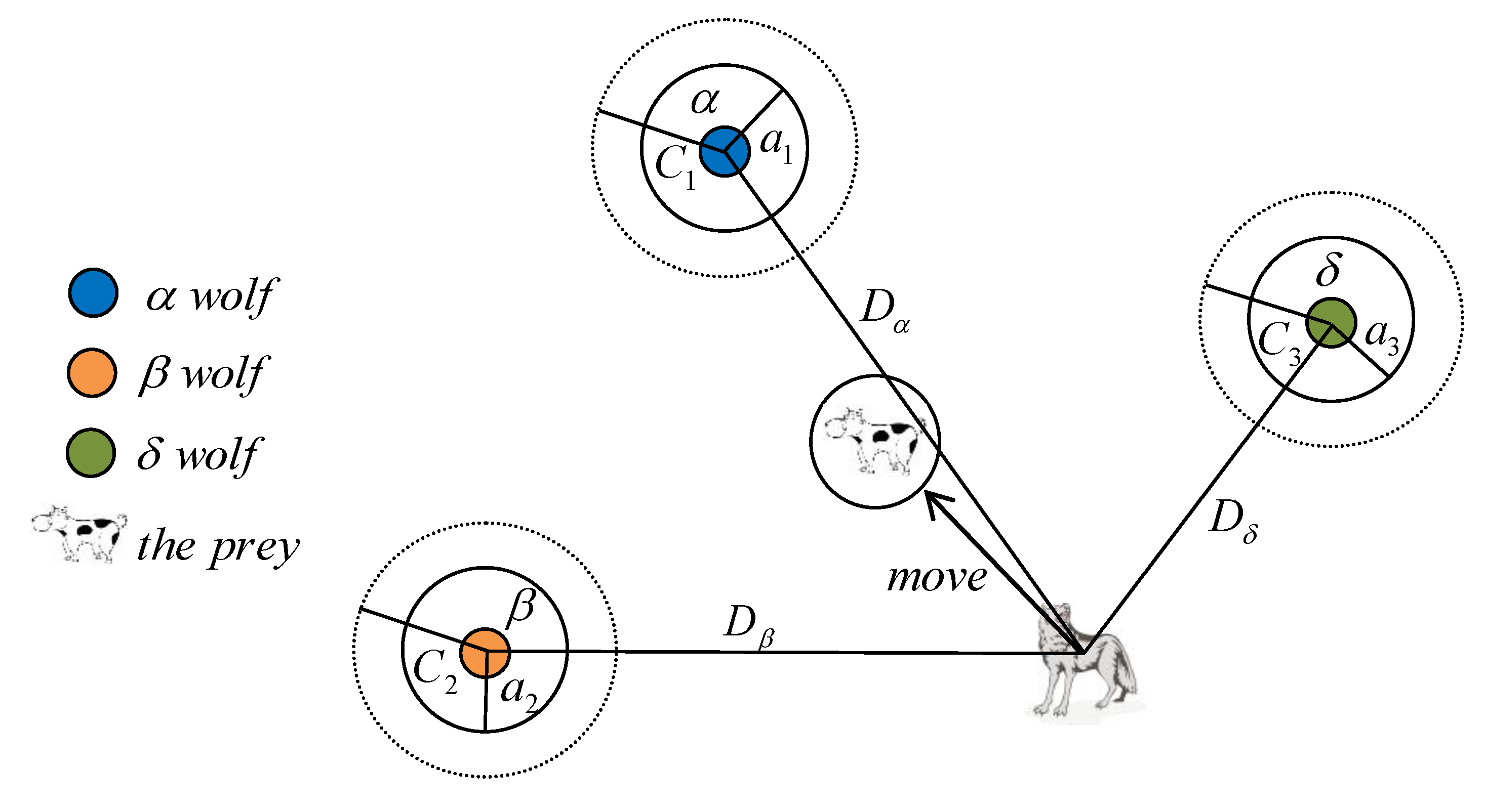
Grey wolves are top-class carnivores dominated by colonies, and their populations have a strict social hierarchy. The grey wolf optimizer algorithm divides the grey wolf population into four levels, α, β, δ, and ω, from high to low, as shown in Figure 1. Hunting (optimization) is mainly guided by α, β, and δ wolves. The remaining ω wolves follow the first three to track and round up. The solutions of the corresponding positions of α, β, and δ wolves are the optimal solution, the sub-optimal solution, and the third optimal solution.

3.1.2. Encircling Prey

In the process of optimization, the grey wolf population finds the best path for hunting by encircling the prey, and defines the distance vector D of the position of the prey and the grey wolf for the mathematical model involved:
D = | C X p ( t ) = X ( t ) | ,
X ( t + 1 ) = X p ( t ) A D ,
a ( t ) = 2 ( 1 t / M ) ,
C = 2 r 2 ,
A = 2 a r 1 a .
among them X p ( t ) and X ( t ) indicate the position of the prey after the t-th iteration and the position of the grey wolf individual, respectively; A and C represent coefficient vectors; r1 and r2 are random numbers between [0, 1]; and a linearly decrements from 2 to 0 as the number of iterations increases during the iteration.

3.1.3. Attack Prey

The grey wolf has the ability to identify the position of the prey and attack the prey. The hunting process is completed by the α, β, and δ wolves guiding the wolves to move. α, β, and δ wolves then choose whether to update their positions through feedback from ω wolf. Their location updating formulas are as follows:
{ D α = | C 1 X α ( t ) = X ω ( t ) | , D β = | C 2 X β ( t ) = X ω ( t ) | , D δ = | C 3 X δ ( t ) = X ω ( t ) | .
{ X 1 = X α A 1 D α , X 2 = X β A 2 D β , X 3 = X δ A 3 D δ .
X ω ( t + 1 ) = ( X 1 + X 2 + X 3 ) / 3 .
among them: Dα, Dβ, and Dδ respectively represent the distance between the search individual (ω wolf) and the α, β and δ wolves; X1, X2, and X3 indicate, respectively, that α, β, and δ wolves guide the direction of individual (ω wolf) movement; Xω(t + 1) indicates the position of the grey wolf individual after updating.
Figure 2 illustrates the above mode formula by giving an illustration of the position at which candidate solution or search individual (ω wolf) updates its position under the guidance of α, β, and δ wolves in a two-dimensional search space. As shown in Figure 2, the random circle range defined by α, β, and δ wolves is the last position of the solution to be selected. That is to say, other wolves choose to update their positions around the prey after the α, β, and δ wolves estimate the position of the prey.

3.2. Algorithmic Flow of Grey Wolf Optimizer

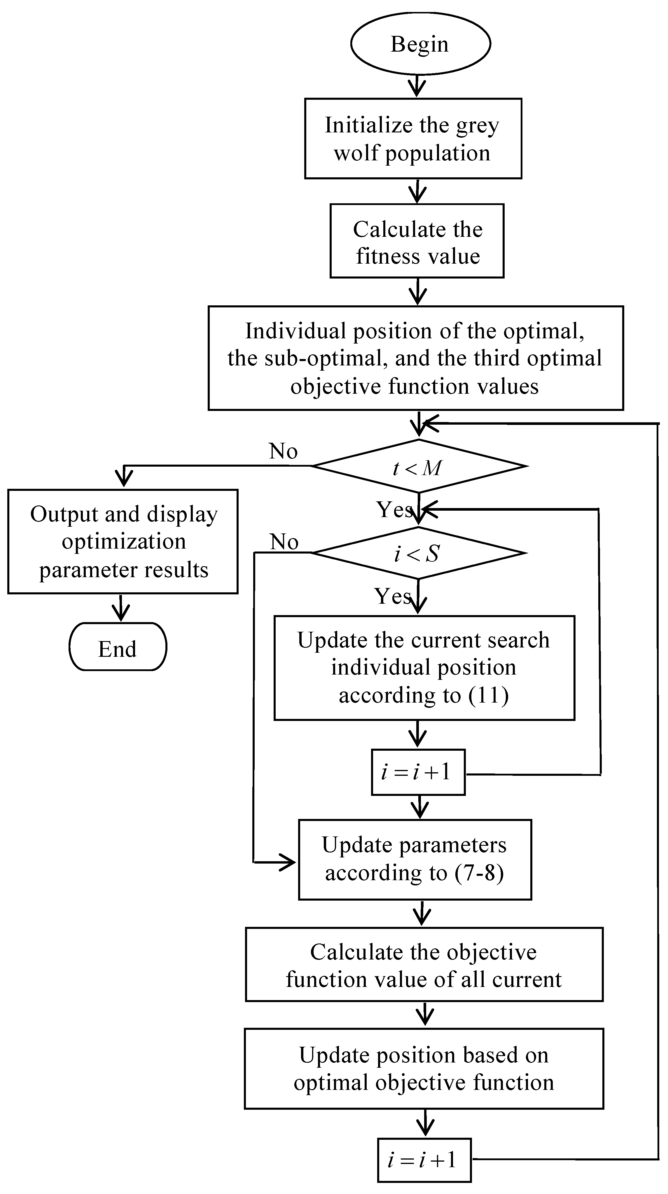
The steps of the grey wolf optimizer algorithm are as follows, and the flow chart of the algorithm is shown in Figure 3.
(1) Initialize the algorithm parameters, set the maximum number of iterations M, and generate parameters such as a, C, and A, and generate the S initial wolf group: Xi (i = 0, 1, …, m).
(2) Record the optimal, the sub-optimal, and the third optimal objective function values corresponding to the positions of the grey wolf individuals, respectively assigned to Xα, Xβ, and Xδ.
(3) Calculate the distance between the search individuals (ω wolf) and the α, β and δ wolves according to Equation (10). Adjust the direction in which the search individuals (ω wolf) move according to Equation (11). The updated position of the grey wolf individuals is calculated according to Equation (12).
(4) Update parameters A, C according to Equations (7)–(9).
(5) Calculate the objective function values of all grey wolf individuals after being updated, and re-determine Xα, Xβ, and Xδ.
(6) Iterate according to t = t + 1, if t < M, then jump to step 4); if t = M, the iteration is terminated, output the optimal solution Xα, and the algorithm ends.

4. Degree Reduction of SG-Bézier Curves with the Grey Wolf Optimizer

4.1. The Basic Idea of SG-Bézier Curve Degree Reduction

Let { P j } j = 0 n be a given series of real numbers, thereby determining the SG-Bézier curve of degree n:
P ( t ) = j = 0 n P j l j , n ( t ) ,
the so-called degree reduction refers to seeking the real numbers { Q j } j = 0 m , so that its corresponding low-mth-degree SG-Bézier curve:
Q ( t ) = j = 0 m Q j l j , m ( t ) ,
meets the condition:
max 0 t 1 d ( P ( t ) , Q ( t ) ) = max 0 t 1 P ( t ) Q ( t ) 2 = min .
The degree reduction problems can be transformed into the following parameter constrained optimization problems:
f ( P , Q , t ; ω , λ j , μ j ) = min max 0 t 1 d ( P ( t ) , Q ( t ) ) s . t .   P , Q R d , 0 ω 1 , λ 0 = μ 0 = 0 , 0 λ j , μ j ( n + 1 j ) ( j = 1 , 2 , , [ n / 2 ] + 1 ) , t [ 0 , 1 ]
where P, Q are the control point vectors of the curve before and after the degree reduction, ω is the global shape parameter, and λ and μ are the local shape control parameters.

4.2. Initialization of the Grey Wolf Population

The population of this paper is consisted of feasible solutions to control points of SG-Bézier curves after degree reduction. To initialize the population, first generate a random number αj ∈ [0, 1] (j = 0, 1, …, m), and then use the following equation to find the control points on the interval [Pmin, Pmax]:
Qj = Pmin + αj(PmaxPmin), j = 0, 1, ..., m,
where Qj is the initial control points of the degree-reduced SG-Bézier curves Q(t), Pmin = (xmin, ymin), Pmax = (xmax, ymax). When the endpoints satisfy the C0 constraint, taking Q0 = P0 and Qm = Pn to ensure the endpoints interpolation; when the endpoints satisfy the C1 constraint, we have:
Q 0 = P 0 , Q m = P n , Q 1 = P 0 + n + ω ω λ 1 m + ω ω λ 1 ( P 1 P 0 ) , Q m 1 = P n n + ω ω μ 1 m + ω ω μ 1 ( P n P n 1 ) .

4.3. Selection of Fitness Function

Each individual of the population has an adaptation value. The better the individual’s nature, the greater the fitness value, and the greater the possibility of breeding the next generation. In order to satisfy the approximate conditions of the SG-Bézier curves, the fitness function is selected as:
f ( t ) = max P ( t ) Q ( t ) = ( j = 0 s d ( P ( t j ) Q ( t j ) ) 2 ) 1 / 2 ,
where d(P(tj),Q(tj)) is Euclidean distance, P(tj) and Q(tj)(j = 0, 1, …, s) are the different points on the SG-Bézier curves before and after degree reduction, respectively.

4.4. The Algorithm Description for Degree Reduction of SG-Bézier Curves

In this paper, the control points of the degree reduction curves are used as the position information of the grey wolves. When the grey wolves constantly update their position after judging the position of the prey, it is equivalent to continuously updating the control points of the degree reduction curves. Based on the introduction of the GWO algorithm in Section 3, the specific implementation steps for applying the GWO algorithm to degree reduction of SG-Bézier curves are given in Algorithm 1, and Algorithm 2 is the corresponding pseudo code.
Algorithm 1 Grey wolf optimizer algorithm: Steps to the degree reduction of SG-Bézier curves.
Step 1Input the degree and control points sequence of SG-Bézier curves before degree reduction {P0, P1, …, Pn}.
Step 2Draw SG-Bézier curve before degree reduction and its control polygon.
Step 3Initialize the parameters, set the population size and the maximum number of iterations MaxIter, determine the number of points on the curve selected in the error analysis before and after the reduction, and give the upper and lower bounds of the search individual information dimension and the search individual information dimension.
Step 4According to Equation (17), generate the initial population Qj(j = 0, 1, …, m).
Step 5According to Equation (19), calculate the fitness value of the grey wolf individual, rank all the fitness values, and record the position Qα, Qβ, Qδof the optimal grey wolf α, the sub-optimal grey wolf β and the third optimal grey wolf ω.
Step 6According to Equation (12), update the position of the current grey wolf.
Step 7Update parameters a, A and C by Equations (7)–(9).
Step 8Calculate the fitness values of all grey wolves after being updated, and determine the new Qα, Qβ and Qδ.
Step 9To determine whether the maximum number of iterations is reached, yes, execute Step 10; No, repeat Step 5Step 9.
Step 10Output optimization parameter result Qα.
Step 11Draw SG-Bézier curve and its control polygon after degree reduction.
Algorithm 2 The pseudo-code of the GWO algorithm: Degree reduction of SG-Bézier curve
Input Parameters: s: Population size;
d: Dimensions of searching individuals;
lb: The lower bound of searching individual dimension;
ub: The upper bound of searching individual dimension;
N: The number of points on the curve selected during error analysis before and after the reduction;
m: Maximum number of iterations;
01wolf population Q j ( j = 1 , 2 , , m ) initialization(wolf_size);
02fitness evaluate(wolf population); /*Calculating individual fitness of grey wolf*/
03while (evaluation_number<max_evaluation_number) do/*Termination condition*/
04   Q α , Q β , Q δ select the first best three wolves(wolf population); /*Select the optimal, sub-optimal, and second optimal wolf*/
05  while (i < m) do
06  new position of the wolf update(the current wolf); /*Update the location of the current search individuals*/
07  evaluation_number + 1;
08 end
09 update(a,A,C)
10 fitness evaluate(new position of the wolf);
11 evaluation_number + 1;
12end
13 Q α select the best wolf(the entire wolves);
14output Q α

5. Examples of Degree Reduction Approximation Curves

In this paper, a large number of numerical studies are carried out to verify the correctness of the algorithm. The experimental environment is MATLAB language (MATLAB R2011a, MathWokrs Corporation, Natick, MA, USA), the operating system is Windows 7 (Windows 7, Microsoft Corporation, Redmond, WA, USA), with an E5400 2.7 Ghz CPU, and 4 GB RAM. Here we take the population size of grey wolves as 20 and the maximum number of iterations as 300. The following examples of applying GWO algorithm to SG-Bézier curves. The error formula of degree reduction is as follows:
ε = d ( P ( t ) , Q ( t ) ) = 0 1 P ( t ) Q ( t ) 2 2 d t .
Example 1.
Given shape parameters and control point coordinates:
ω * = 0 ; λ 1 * = 3 , λ 2 * = 3 ; λ 3 * = 3 ; μ 1 * = 3 , μ 2 * = 3 ; μ 3 * = 3 ; { P 0 * = ( 0.1 , 0 ) , P 1 * = ( 0 , 0.1 ) , P 2 * = ( 0.05 , 0.2 ) , P 3 * = ( 0.3 , 0.3 ) , P 4 * = ( 0.55 , 0.2 ) , P 5 * = ( 0.6 , 0.1 ) , P 6 * = ( 0.5 , 0 ) } ,
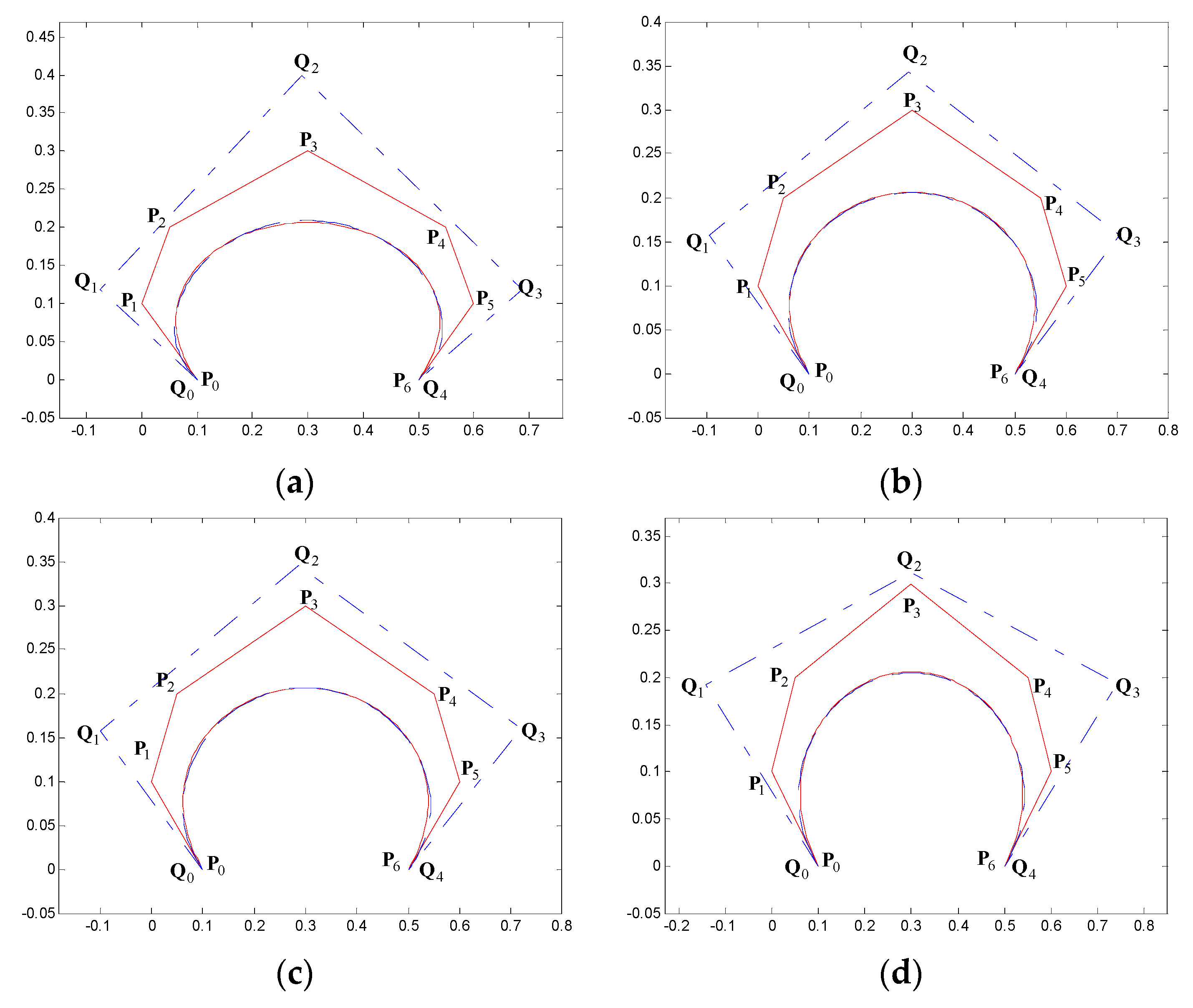
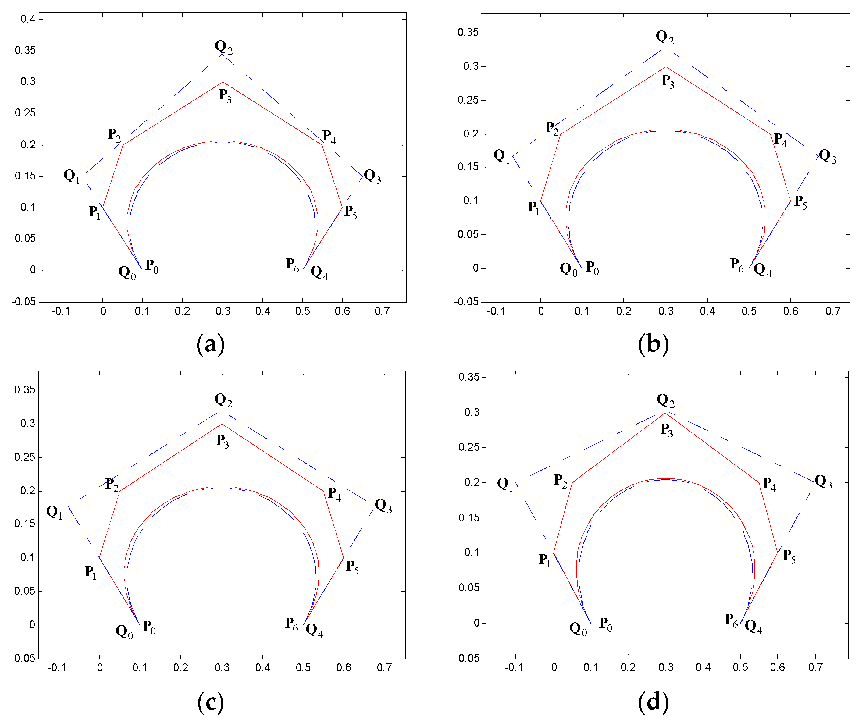
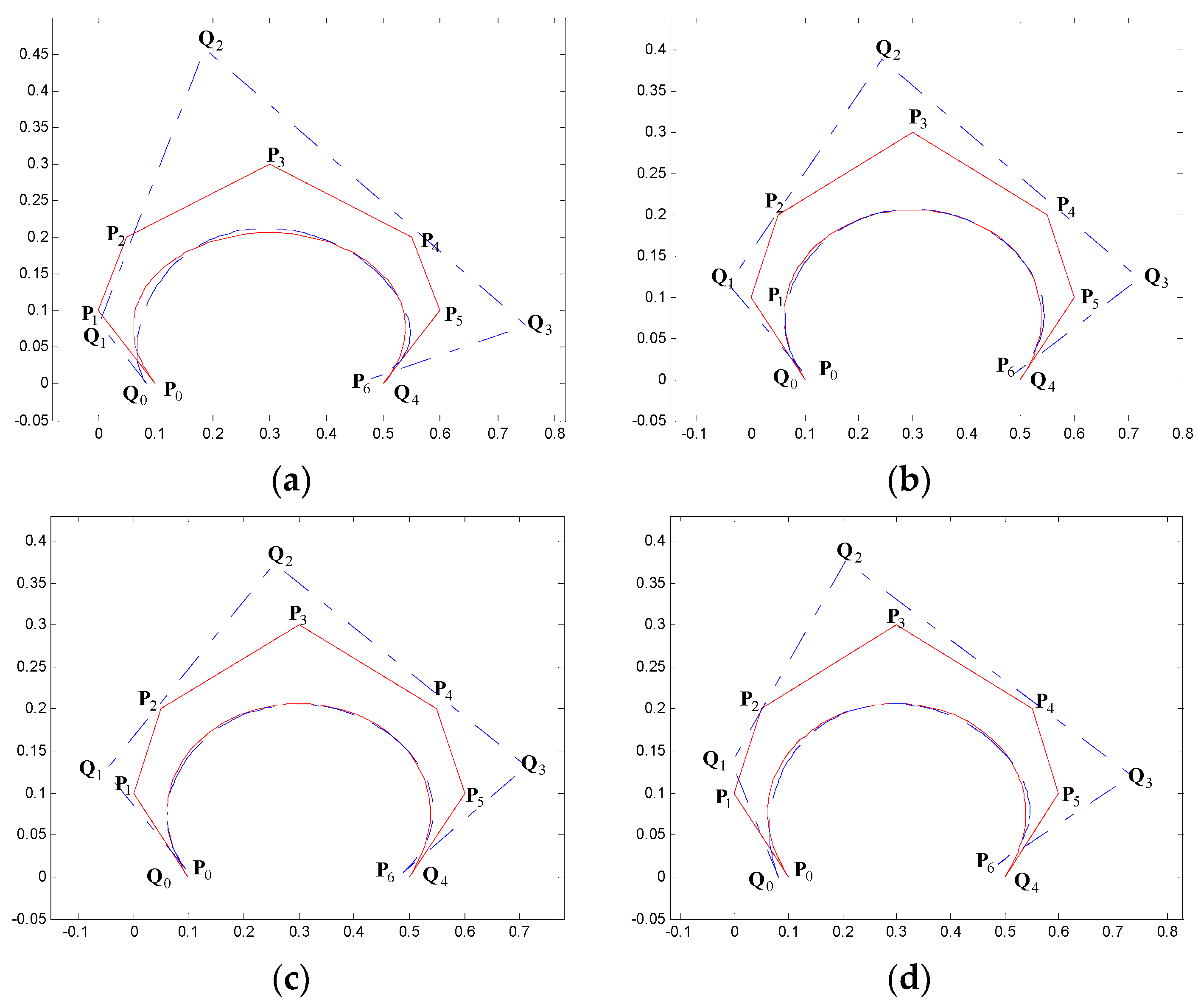
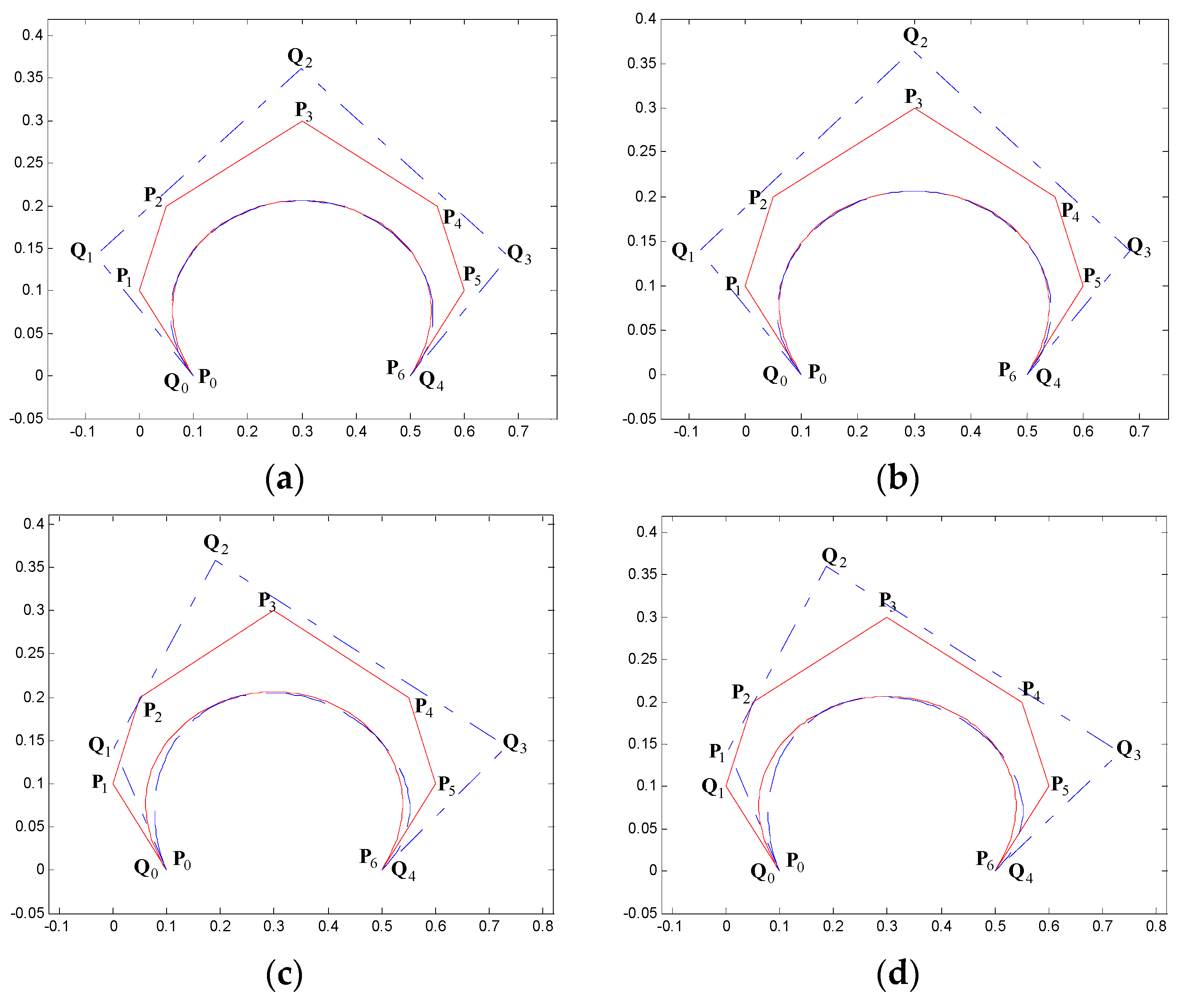
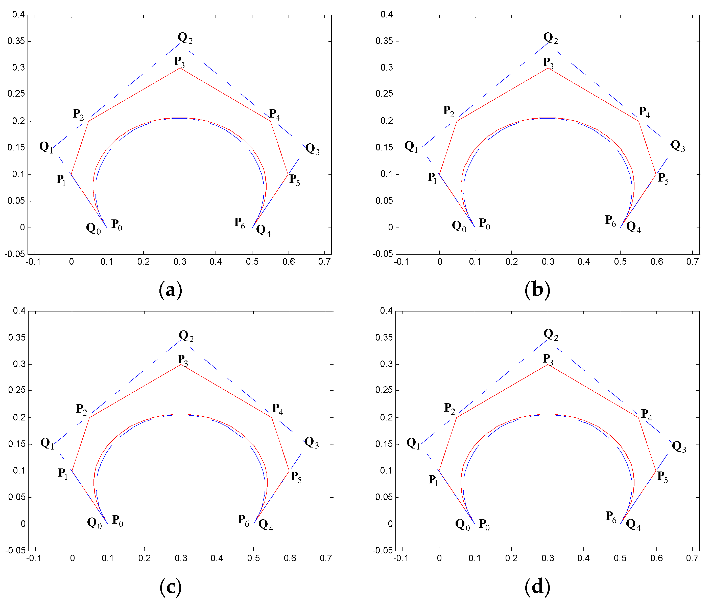
construct SG-Bézier curves (blue solid line) of degree 6, and its degree reduced SG-Bézier curves of degree 4 (red dot line) under unconstrained and constrained conditions of C0 and C1. Under each kind of constraints, two different situations are given: changing global shape parameters (Figure 4, Figure 5 and Figure 6) and changing local shape parameters (Figure 7, Figure 8 and Figure 9). The errors of the curves after the degree reduction are shown in Table 2 and Table 3, respectively.
Example 2.
Given shape parameters and control point coordinates:
ω * = 0 ; λ 1 * = 3 , λ 2 * = 3 ; λ 3 * = 3 ; λ 4 * = 3 ; λ 5 * = 3 ; μ 1 * = 3 , μ 2 * = 3 ; μ 3 * = 3 ; μ 4 * = 3 ; { P 0 * = ( 0.5 , 0 ) , P 1 * = ( 0.8 , 0.3 ) , P 2 * = ( 0.65 , 0.7 ) , P 3 * = ( 0.1 , 1 ) , P 4 * = ( 0.6 , 1.1 ) , P 5 * = ( 1.3 , 1 ) , P 6 * = ( 1.85 , 0.7 ) , P 7 * = ( 2 , 0.3 ) , P 8 * = ( 1.7 , 0 ) }
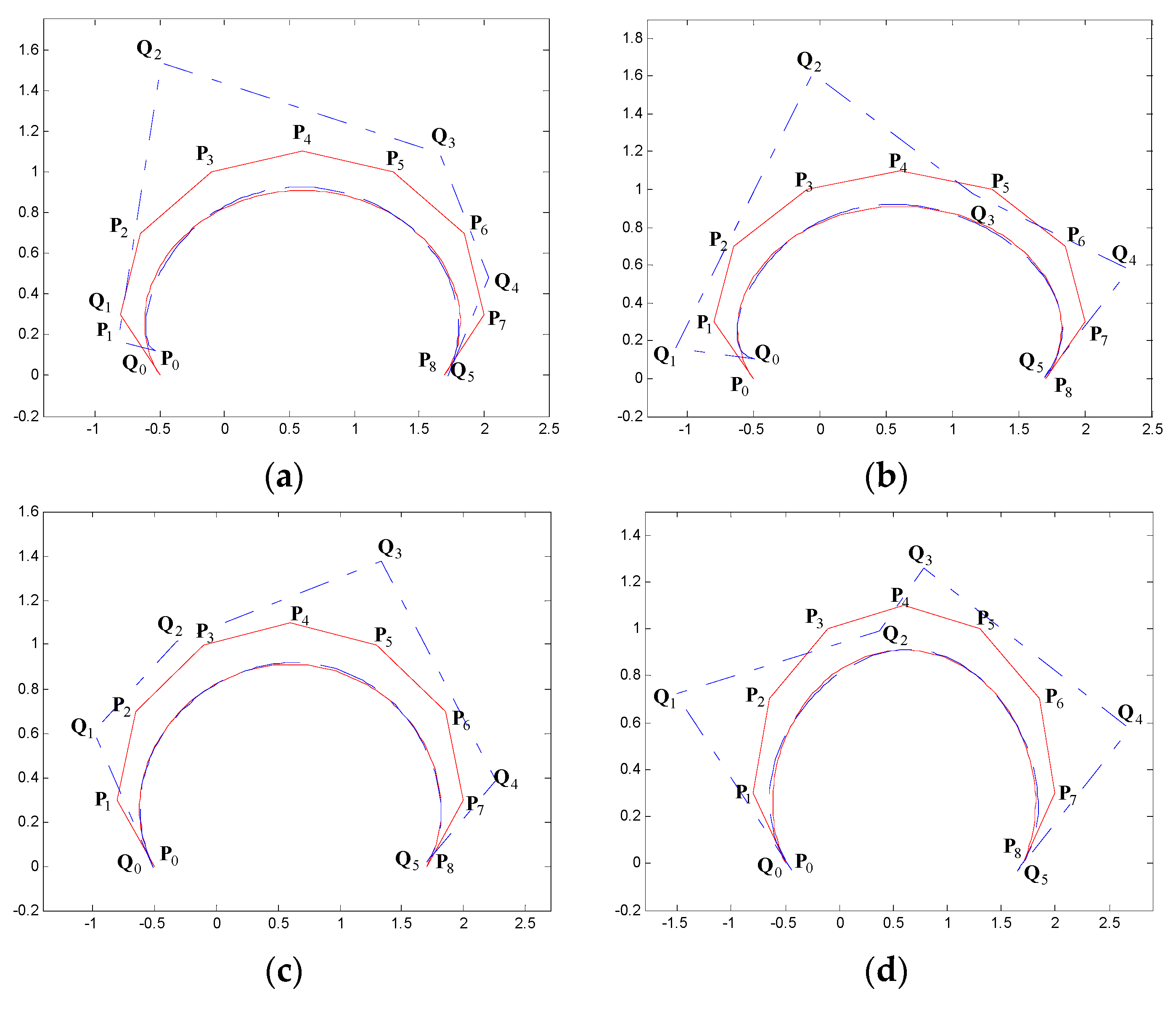
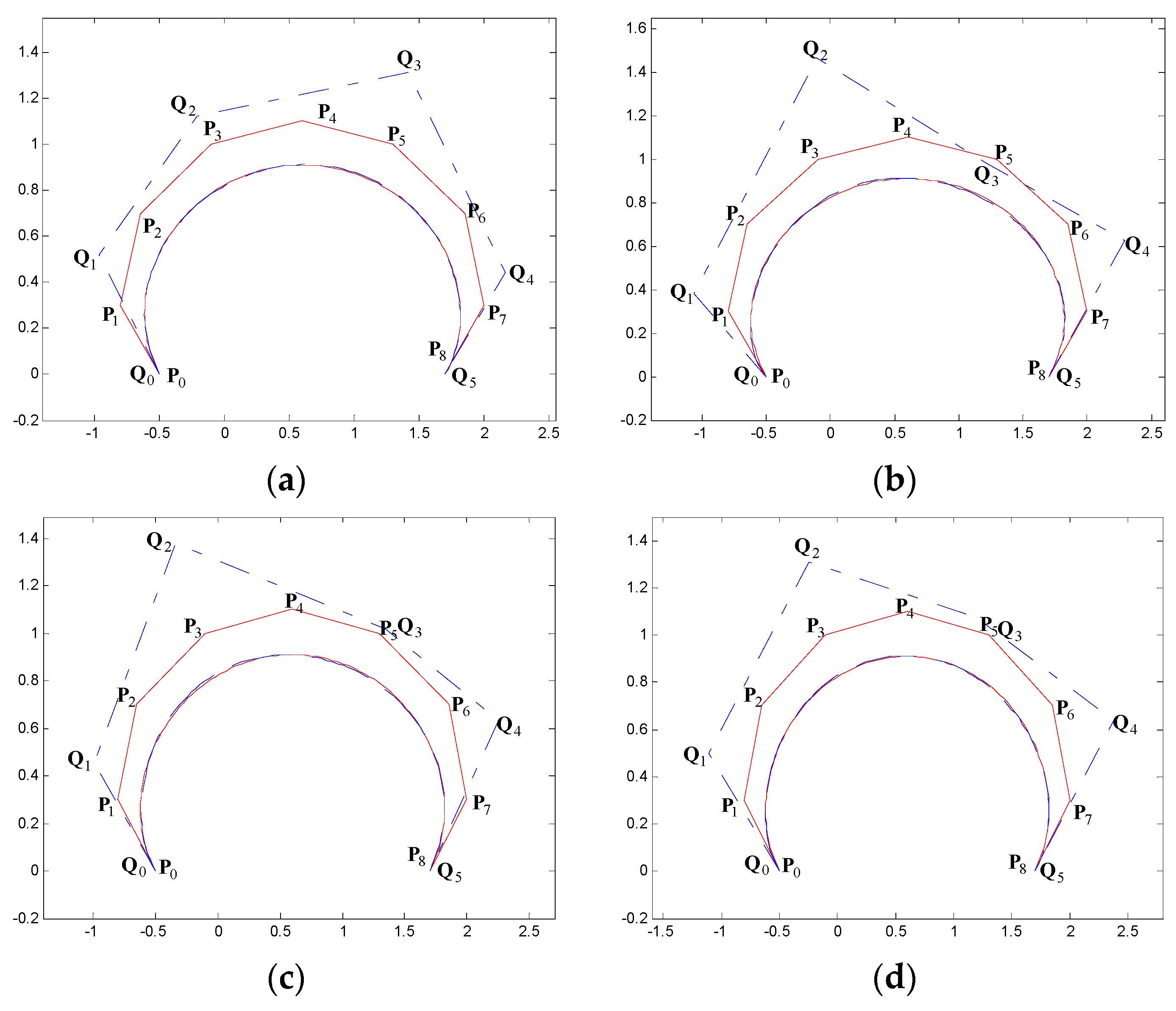
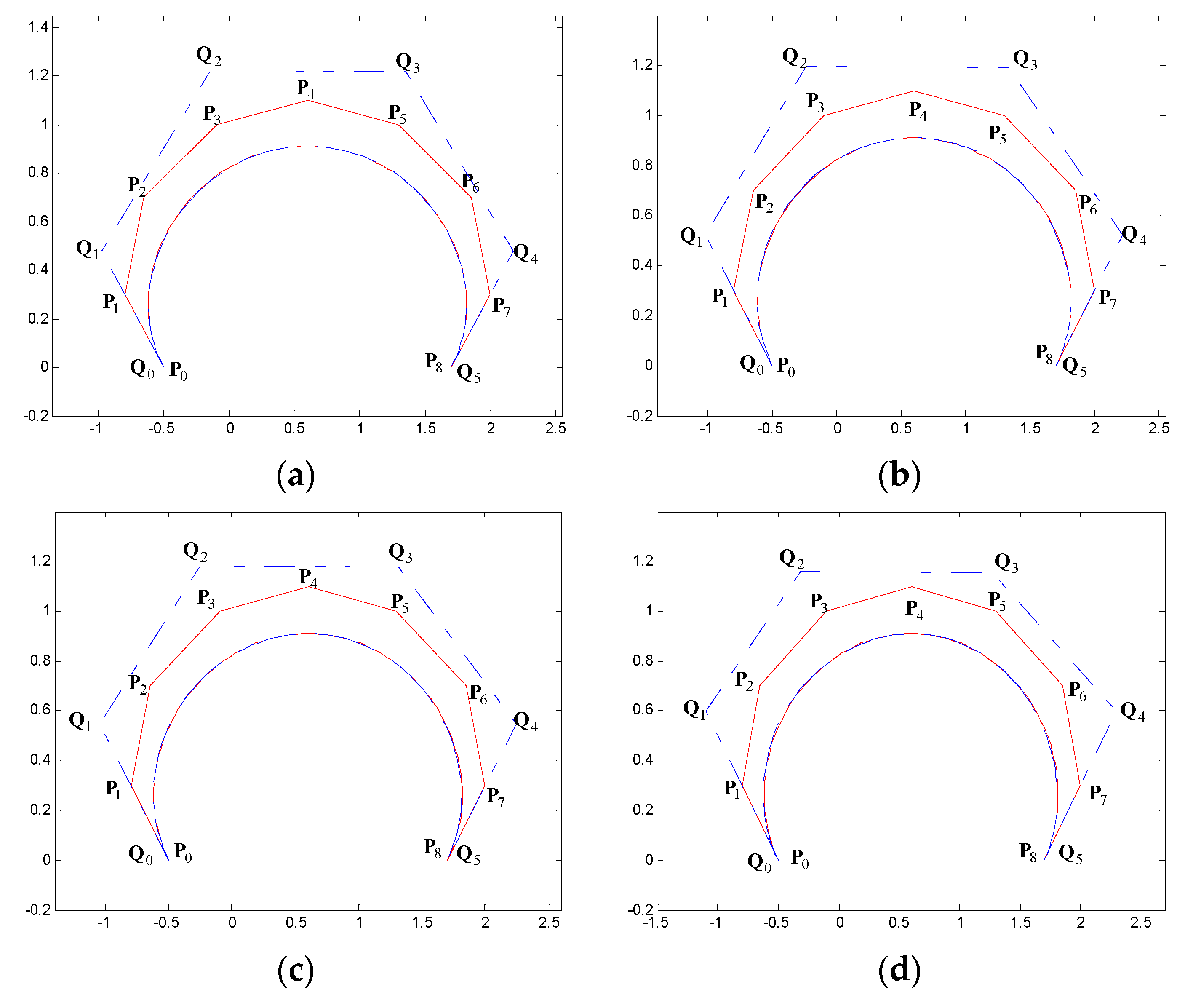
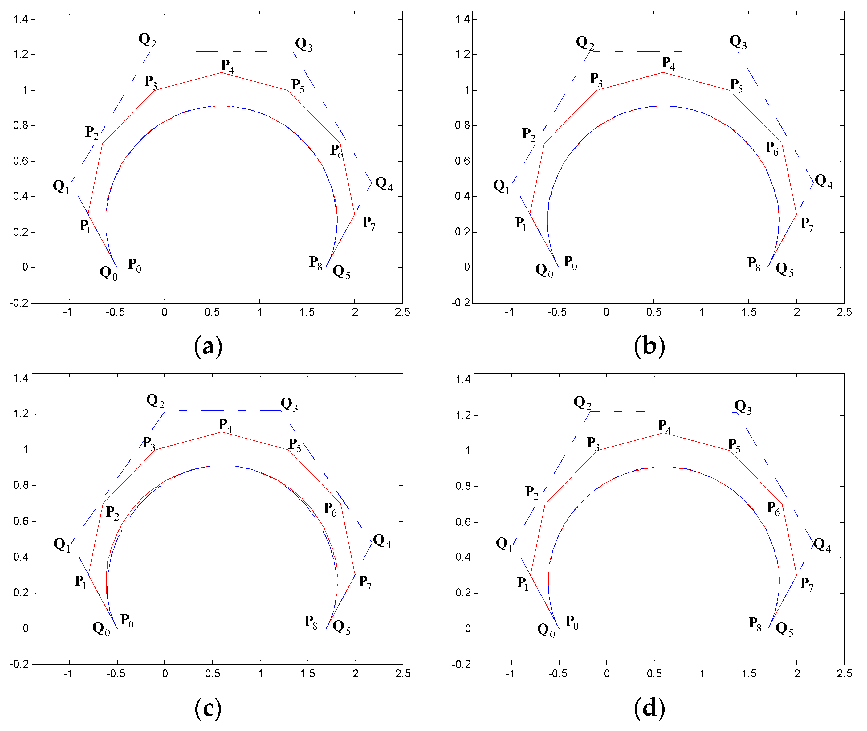
construct SG-Bézier curves (blue solid line) of degree 8, and its degree reduce SG-Bézier curves of degree 5 (red dot line) under unconstrained and constrained conditions of C0 and C1. Under each kind of constraints, two different situations are given: changing global shape parameters (Figure 10, Figure 11 and Figure 12) and changing local shape parameters (Figure 13, Figure 14 and Figure 15). The errors of the curves after the degree reduction are shown in Table 4 and Table 5, respectively.
Example 3.
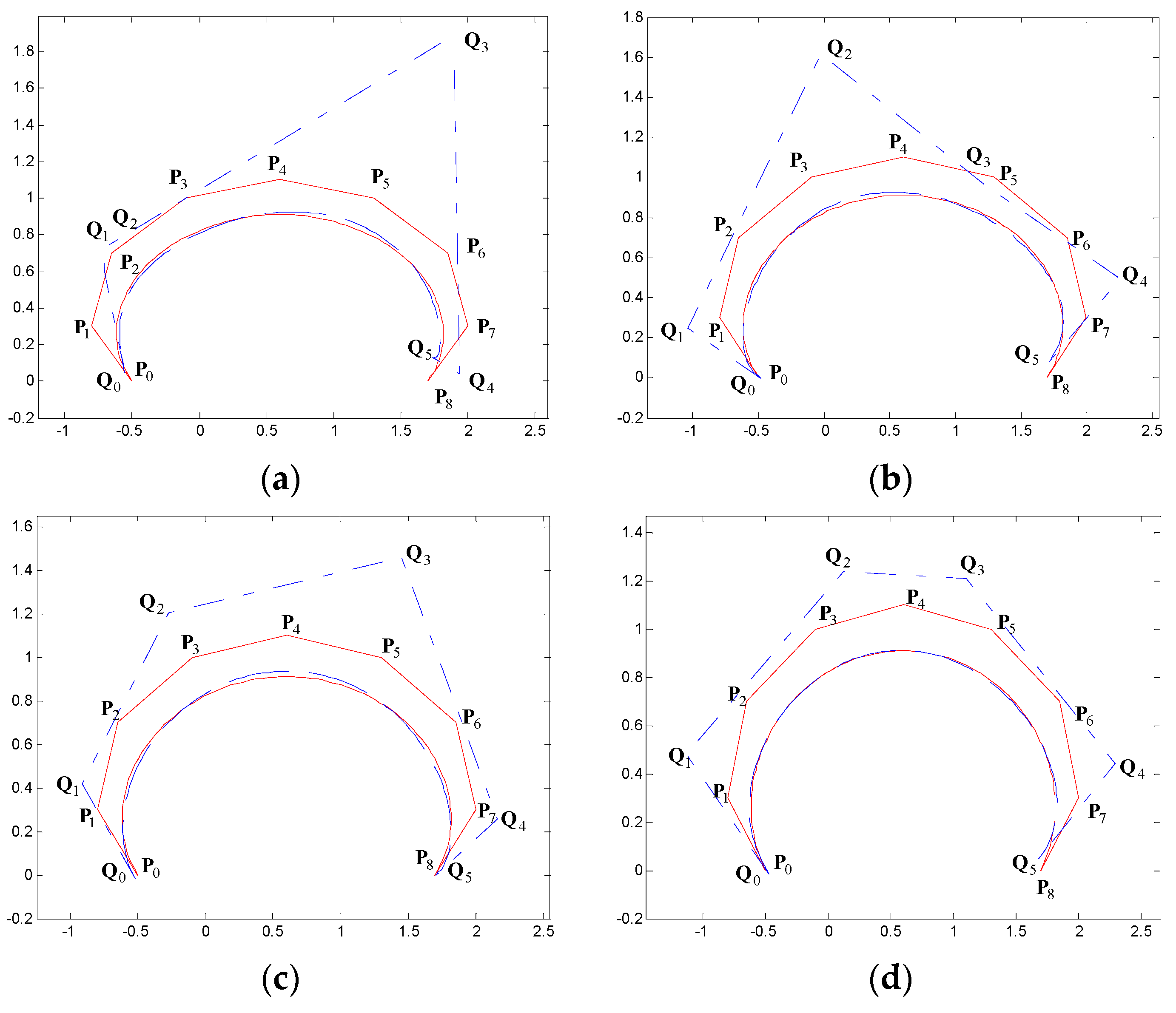
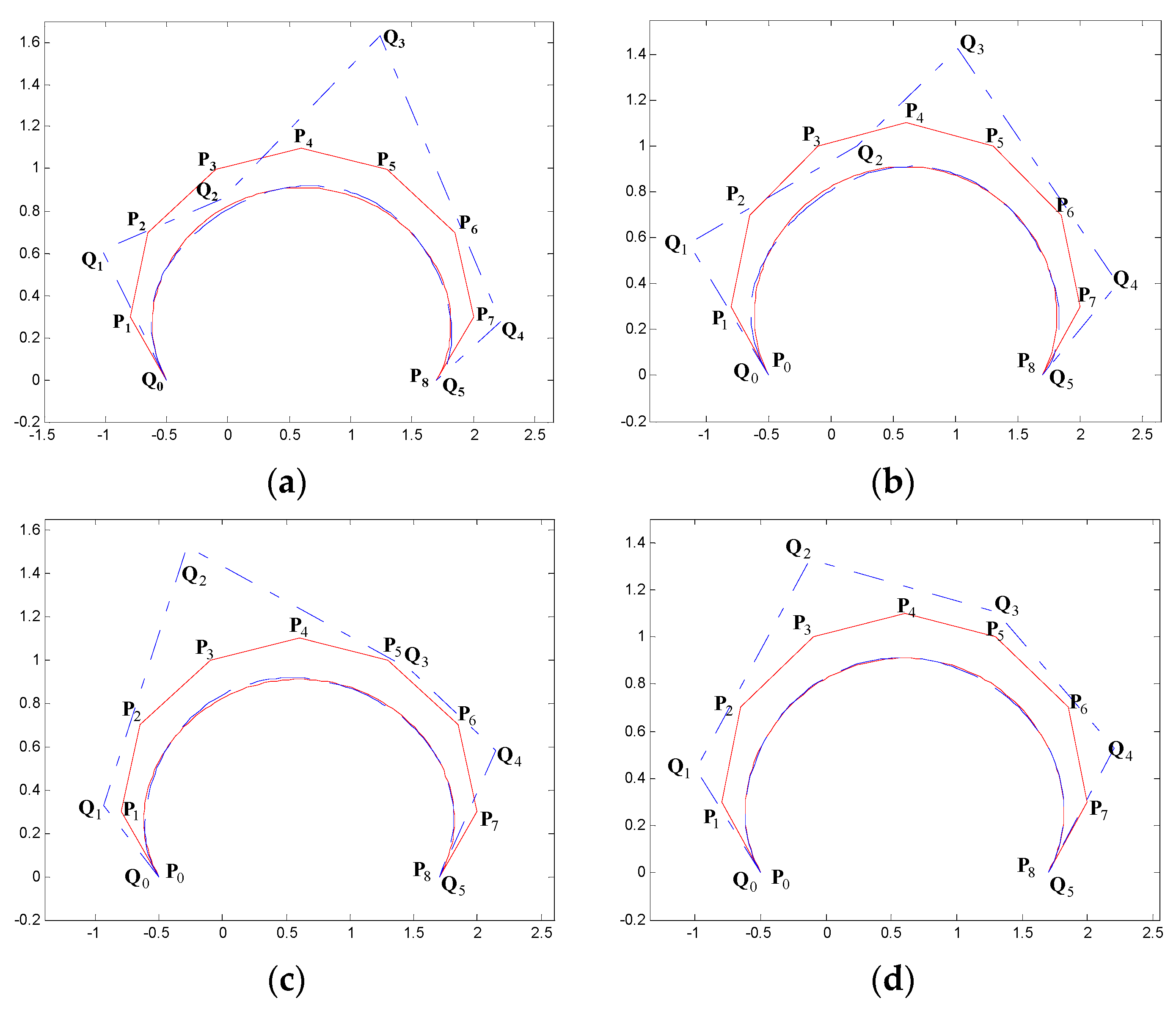
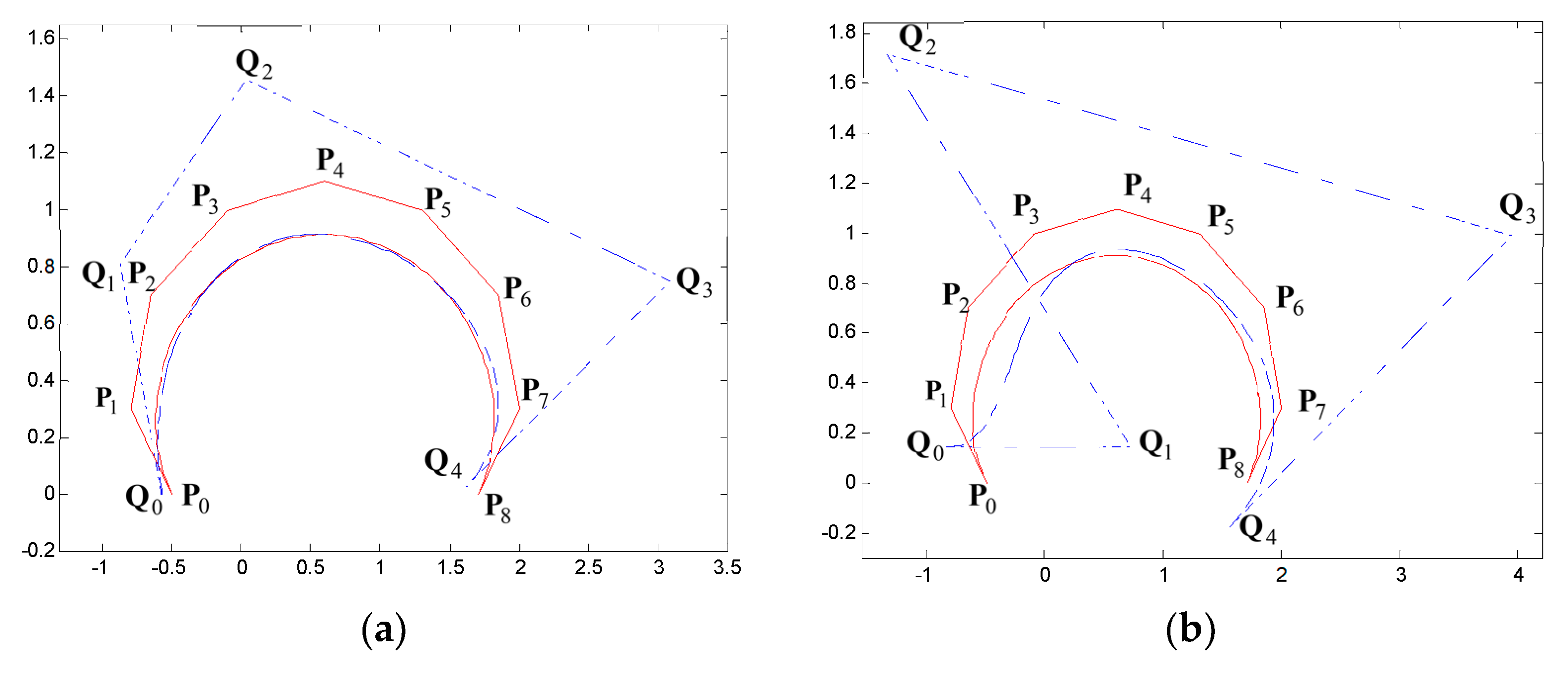
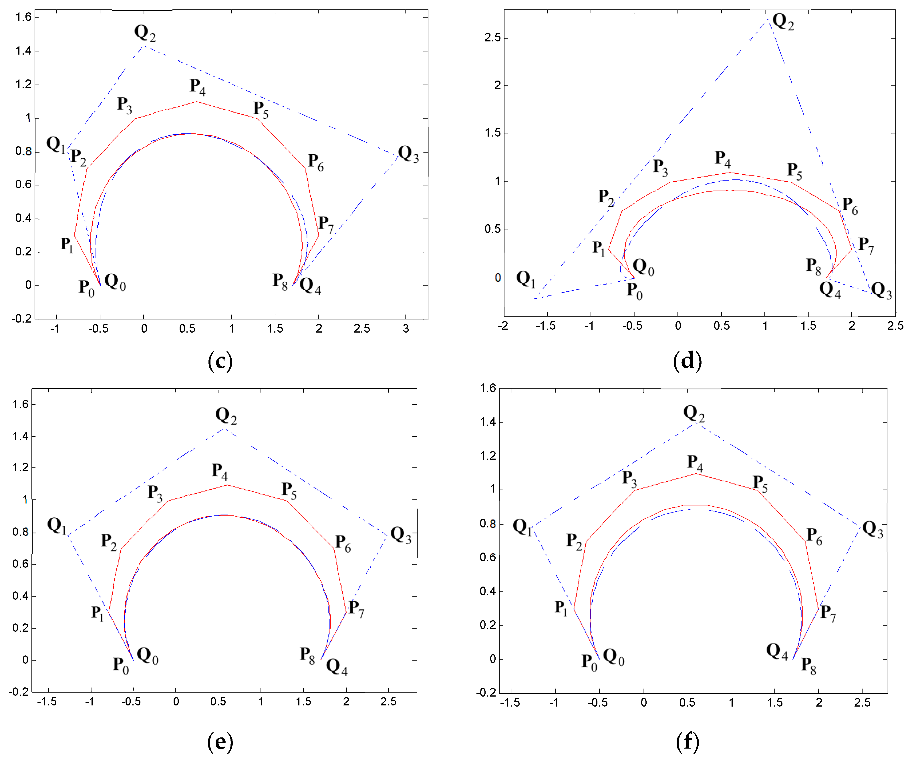
For the degree reduction of traditional Bézier curves, scholars have done a lot of related researches; see [22,23,24,25,26,27,28,29,30]. Nevertheless, up to now, the related work about degree reduction of SG-Bézier curves has not been studied. Owing to the complexity of SG-Bézier curves, the degree reduction method of traditional SG-Bézier curves isn’t able to solve its problem of approximate degree reduction. On this account, in this paper, we study the approximate degree reduction of SG-Bézier curves using the grey wolf optimizer algorithm. In order to verify the degree reduction effect of the proposed method, in Example 3, we gave a comparison between the proposed method (or GWO method, for short) and GA method. Here, the GA method refers to SG-Bézier curves degree reduction based on the genetic algorithm, that is, the genetic algorithm in [36] is used to solve the degree reduction model of SG-Bézier curves in Equation (16). The initial parameters of genetic algorithm are set as follows: the initial population size is 100, the number of iterations is 200, the crossover probability is 0.5 and the mutation probability is 0.1. Figure 16 shows the comparison of degree reduction effects between GWO method and GA method under different constraints. In Figure 16, the curve before degree reduction is an 8-th SG-Bézier curve whose control points and shape parameters are the same as those in Example 2; the curve after degree reduction is a 4-th SG-Bézier curve. Table 6 shows the error comparison of the two degree reduction methods in Figure 16. Obviously, as can be seen from Figure 16 and Table 6, the GWO method is better than the GA method, which further demonstrates the effectiveness of the proposed method.

6. Conclusions

Combining the geometric properties of SG-Bézier curves with the grey wolf optimizer algorithm, this paper studied degree reduction of SG-Bézier curves under unrestricted condition and constraint condition of C0 and C1. These examples fully demonstrate the characteristics of the global optimization of the grey wolf optimizer algorithm in the process of degree reduction. That is to say this method is applicable for CAD/CAM modeling systems. The research on how to utilize the GWO algorithm [32,33,34,35] or genetic algorithm [36] to solve the model of curve shape optimization, which takes the shape parameters as the optimization variables, will be addressed in our future work.

Author Contributions

All authors contributed equally to the writing of this paper. All authors read and approved the final manuscript.

Funding

This work is supported by the National Natural Science Foundation of China (grant no. 51875454).

Acknowledgments

We thank to the anonymous reviewers for their insightful suggestions and recommendations, which led to the improvements of presentation and content of the paper.

Conflicts of Interest

The authors declare that there is no conflict of interests regarding the publication of this paper.

References

  1. Farin, G. Curves and Surfaces for CAGD: A Practical Guide, 5th ed.; Academic Press: San Diego, CA, USA, 2002. [Google Scholar]
  2. Mamar, E. Shape preserving alternatives to the rational Bézier model. Comput. Aided Geom. Des. 2001, 18, 37–60. [Google Scholar] [CrossRef]
  3. Qinyu, C.; Guozhao, W. A class of Bézier-like curves. Comput. Aided Geom. Des. 2003, 20, 29–39. [Google Scholar]
  4. Oruc, H.; Phillips, G.H. q-Bézier Bernstein polynomials and Bézier curves. J. Comput. Appl. Math. 2003, 151, 1–12. [Google Scholar] [CrossRef]
  5. Hu, G.; Wu, J.L.; Qin, X.Q. A new approach in designing of local controlled developable H-Bézier surfaces. Adv. Eng. Softw. 2018, 121, 26–38. [Google Scholar] [CrossRef]
  6. Han, X. Cubic trigonometric polynomial curves with a shape parameter. Comput. Aided Geom. Des. 2004, 21, 535–548. [Google Scholar] [CrossRef]
  7. Wang, G.; Yang, Q. Planar cubic hybrid hyperbolic polynomial curve and its shape classification. Prog. Nat. Sci. 2004, 14, 41–46. [Google Scholar] [CrossRef]
  8. Zhang, J.; Krause, F.L.; Zhang, H. Unifying C-curves and H-curves by extending the calculation to complex numbers. Comput. Aided Geom. Des. 2005, 22, 865–883. [Google Scholar] [CrossRef]
  9. Hu, G.; Bo, C.C.; Qin, X.Q. Continuity conditions for tensor product Q-Bézier surfaces of degree (m, n). Comput. Appl. Math. 2018, 37, 4237–4258. [Google Scholar] [CrossRef]
  10. Han, X.A.; Ma, Y.C.; Huang, X. The cubic trigonometric Bézier curve with two shape parameters. Appl. Math. Lett. 2009, 22, 226–231. [Google Scholar] [CrossRef]
  11. Han, X.A.; Huang, X.; Ma, Y.C. Shape analysis of cubic trigonometric Bézier curves with a shape parameter. Appl. Math. Comput. 2010, 217, 2527–2533. [Google Scholar] [CrossRef]
  12. Rachid, A.; Yusuke, S.; Taishin, N. Gelfond-Bézier curves. Comput. Aided Geom. Des. 2013, 30, 199–225. [Google Scholar]
  13. Qin, X.Q.; Hu, G.; Yang, Y.; Wei, G. Construction of PH splines based on H-Bézier curves. Appl. Math. Comput. 2014, 238, 460–467. [Google Scholar] [CrossRef]
  14. Farin, G. Class a Bézier curves. Comput. Aided Geom. Des. 2006, 23, 573–581. [Google Scholar] [CrossRef]
  15. Han, X.A.; Ma, Y.; Huang, X. A novel generalization of Bézier curve and surface. J. Comput. Appl. Math. 2008, 217, 180–193. [Google Scholar] [CrossRef]
  16. Yang, L.; Zeng, X.M. Bézier curves and surfaces with shape parameter. Int. J. Comput. Math. 2009, 86, 1253–1263. [Google Scholar] [CrossRef]
  17. Hu, G.; Cao, H.X.; Zhang, S.X.; Guo, W. Developable Bézier-like surfaces with multiple shape parameters and its continuity conditions. Appl. Math. Model. 2017, 45, 728–747. [Google Scholar] [CrossRef]
  18. Yan, L.; Liang, J. An extension of the Bézier model. Appl. Math. Comput. 2011, 218, 2863–2879. [Google Scholar] [CrossRef]
  19. Qin, X.Q.; Hu, G.; Zhang, N.J.; Shen, X.; Yang, Y. A novel extension to the polynomial basis functions describing Bézier curves and surfaces of degree n with multiple shape parameters. Appl. Math. Comput. 2013, 223, 1–16. [Google Scholar] [CrossRef]
  20. Hu, G.; Wu, J.L.; Qin, X.Q. A novel extension of the Bézier model and its applications to surface modeling. Adv. Eng. Softw. 2018, 125, 27–54. [Google Scholar] [CrossRef]
  21. Hu, G.; Bo, C.; Wu, J.L.; Wei, G.; Hou, F. Modeling of free-form complex curves using SG-Bézier curves with constraints of geometric continuities. Symmetry 2018, 10, 545. [Google Scholar] [CrossRef]
  22. Zhao, Y. Research on degree reduction of C-Bézier curves based on generalized inverse matrix. Netw. Secur. Technol. Appl. 2010, 10, 38–40. [Google Scholar]
  23. Chen, G.; Wang, G.J. Degree reduction approximation of Bézier curves by generalized inverse matrices. J. Comput. Aided Des. Comput. Graph. 2001, 12, 435–439. [Google Scholar]
  24. Cai, H.J.; Wang, G.J. Constrained approximation of rational Bézier curves based on a matrix expression of its end points continuity condition. Comput. Aided Des. 2010, 42, 495–504. [Google Scholar] [CrossRef]
  25. Gospodarczyk, P. Degree reduction of Bézier curves with restricted control points area. Comput. Aided Des. 2015, 62, 143–151. [Google Scholar] [CrossRef]
  26. Ahn, Y.J. Using Jacobi polynomials for degree reduction of Bézier curves with Ck-constraints. Comput. Aided Geom. Des. 2003, 20, 423–434. [Google Scholar] [CrossRef]
  27. Lee, B.G.; Park, Y.; Yoo, J. Application of Legendre-Bernstein basis transformations to degree elevation and degree reduction. Comput. Aided Geom. Des. 2002, 19, 709–718. [Google Scholar] [CrossRef]
  28. Rababah, A.; Lee, B.G.; Yoo, J. A simple matrix form for degree reduction of Bézier curves using Chebyshev-Bernstein basis transformations. Appl. Math. Comput. 2006, 181, 310–318. [Google Scholar] [CrossRef]
  29. Ahn, Y.J.; Lee, B.G.; Park, Y.; Yoo, J. Constrained polynomial degree reduction in the L2-norm equals best weighted Euclidean approximation of Bézier coefficients. Comput. Aided Geom. Des. 2004, 21, 181–191. [Google Scholar] [CrossRef]
  30. Ait-Haddou, R.; Bartoň, M. Constrained multi-degree reduction with respect to Jacobi norms. Comput. Aided Geom. Des. 2016, 42, 23–30. [Google Scholar] [CrossRef] [Green Version]
  31. Lu, J.; Qin, X. Degree reduction of S-λ curves using a genetic simulated annealing algorithm. Symmetry 2019, 11, 15. [Google Scholar] [CrossRef]
  32. Mirjalili, S.; Mirjalili, S.M.; Lewis, A. Grey wolf optimizer. Adv. Eng. Softw. 2014, 69, 46–61. [Google Scholar] [CrossRef]
  33. Saremi, S.; Mirjalili, S.Z.; Mirjalili, S.M. Evolutionary population dynamics and grey wolf optimizer. Neural Comp. Appl. 2015, 26, 1257–1263. [Google Scholar] [CrossRef]
  34. Mirjalili, S. How effective is the Grey Wolf optimizer in training multi-layer perceptrons. Tech. J. Eng. Appl. Sci. 2014, 4, 373–379. [Google Scholar] [CrossRef]
  35. Song, H.; Sulaiman, M.; Mohamed, M. An application of grey wolf optimizer for solving combined economic emission dispatch problems. Int. Rev. Model. Simul. 2014, 7, 838–844. [Google Scholar]
  36. Caponetto, R.; Fortuna, L.; Graziani, S.; Xibilia, M.G. Genetic algorithms and applications in system engineering: A survey. Trans. Inst. Meas. Control 1993, 15, 143–156. [Google Scholar] [CrossRef]
Figure 1. Social hierarchy of grey wolves.
Symmetry 11 01242 g001
Figure 2. Update position of the grey wolf.
Symmetry 11 01242 g002
Figure 3. Flow chart of the GWO algorithm.
Symmetry 11 01242 g003
Figure 4. Degree reduction of SG-Bézier curves of degree 6 under unrestricted condition in Example 5.1; changing global shape parameter. (a) {λ1 = 3, λ2 = 3, λ3 = 3, µ1 = 3, µ2 = 3, µ3 = 3; ω = 0}; (b) {λ1 = 3, λ2 = 3, λ3 = 3, µ1 = 3, µ2 = 3, µ3 = 3; ω = 0.2}; (c) {λ1 = 3, λ2 = 3, λ3 = 3, µ1 = 3, µ2 = 3, µ3 = 3; ω = 0.3}; (d) {λ1 = 3, λ2 = 3, λ3 = 3, µ1 = 3, µ2 = 3, µ3 = 3; ω = 0.5}.
Symmetry 11 01242 g004
Figure 5. Degree reduction of SG-Bézier curve of degree 6 under C0 constraint condition in Example 5.1; changing global shape parameter. (a) {λ1 = 3, λ2 = 3, λ3 = 3, µ1 = 3, µ2 = 3, µ3 = 3; ω = 0}; (b) {λ1 = 3, λ2 = 3, λ3 = 3, µ1 = 3, µ2 = 3, µ3 = 3; ω = 0.2}; (c) {λ1 = 3, λ2 = 3, λ3 = 3, µ1 = 3, µ2 = 3, µ3 = 3; ω = 0.3}; (d) {λ1 = 3, λ2 = 3, λ3 = 3, µ1 = 3, µ2 = 3, µ3 = 3; ω = 0.5}.
Symmetry 11 01242 g005
Figure 6. Degree reduction of SG-Bézier curve of degree 6 under C1 constraint condition in Example 5.1; changing global shape parameter. (a) {λ1 = 3, λ2 = 3, λ3 = 3, µ1 = 3, µ2 = 3, µ3 = 3; ω = 0}; (b) {λ1 = 3, λ2 = 3, λ3 = 3, µ1 = 3, µ2 = 3, µ3 = 3; ω = 0.2}; (c) {λ1 = 3, λ2 = 3, λ3 = 3, µ1 = 3, µ2 = 3, µ3 = 3; ω = 0.3}; (d) {λ1 = 3, λ2 = 3, λ3 = 3, µ1 = 3, µ2 = 3, µ3 = 3; ω = 0.5}.
Symmetry 11 01242 g006
Figure 7. Degree reduction of SG-Bézier curve of degree 6 under unrestricted condition in Example 5.1; changing local shape parameters. (a) {ω = 0, λ2 = 3, µ1 = 3, µ2 = 3; λ1 = 2}; (b) {ω = 0, λ1 = 3, µ1 = 3, µ2 = 3; λ2 = 4}; (c) {ω = 0, λ1 = 3, λ2 = 3, µ2 = 3; µ1 = 2}; (d) {ω = 0, λ2 = 3, µ1 = 3; λ1 = 2, µ2 = 2}.
Symmetry 11 01242 g007
Figure 8. Degree reduction of SG-Bézier curve of degree 6 under C0 constraint condition in Example 5.1; changing local shape parameters. (a) {ω = 0, λ2 = 3, µ1 = 3, µ2 = 3; λ1 = 2}; (b) {ω = 0, λ1 = 3, µ1 = 3, µ2 = 3; λ2 = 4}; (c) {ω = 0, λ1 = 3, λ2 = 3, µ2 = 3; µ1 = 2}; (d) {ω = 0, λ2 = 3, µ1 = 3; λ1 = 2, µ2 = 2}.
Symmetry 11 01242 g008
Figure 9. Degree reduction of SG-Bézier curve of degree 6 under C1 constraint condition in Example 5.1; changing local shape parameters. (a) {ω = 0, λ2 = 3, µ1 = 3, µ2 = 3; λ1 = 2}; (b) {ω = 0, λ1 = 3, µ1 = 3, µ2 = 3; λ2 = 4}; (c) {ω = 0, λ1 = 3, λ2 = 3, µ2 = 3; µ1 = 2}; (d) {ω = 0, λ2 = 3, µ1 = 3; λ1 = 2, µ2 = 2}.
Symmetry 11 01242 g009
Figure 10. Degree reduction of SG-Bézier curve of degree 8 under unrestricted condition in Example 5.2; changing global shape parameter. (a) {λ1 = 3, λ2 = 3, λ3 = 3, µ1 = 3, µ2 = 3; ω = 0}; (b) {λ1 = 3, λ2 = 3, λ3 = 3, µ1 = 3, µ2 = 3; ω = 0.2};(c) {λ1 = 3, λ2 = 3, λ3 = 3, µ1 = 3, µ2 = 3; ω = 0.3};(d) {λ1 = 3, λ2 = 3, λ3 = 3, µ1 = 3, µ2 = 3; ω = 0.5}.
Symmetry 11 01242 g010
Figure 11. Degree reduction of SG-Bézier curve of degree 8 under C0 constraint condition in Example 5.2; changing global shape parameter. (a) {λ1 = 3, λ2 = 3, λ3 = 3, µ1 = 3, µ2 = 3; ω = 0}; (b) {λ1 = 3, λ2 = 3, λ3 = 3, µ1 = 3, µ2 = 3; ω = 0.2}; (c) {λ1 = 3, λ2 = 3, λ3 = 3, µ1 = 3, µ2 = 3; ω = 0.3};(d) {λ1 = 3, λ2 = 3, λ3 = 3, µ1 = 3, µ2 = 3; ω = 0.5}.
Symmetry 11 01242 g011
Figure 12. Degree reduction of SG-Bézier curve of degree 8 under C1 constraint condition in Example 5.2; changing global shape parameter. (a) {λ1 = 3, λ2 = 3, λ3 = 3, µ1 = 3, µ2 = 3; ω = 0}; (b) {λ1 = 3, λ2 = 3, λ3 = 3, µ1 = 3, µ2 = 3; ω = 0.2}; (c) {λ1 = 3, λ2 = 3, λ3 = 3, µ1 = 3, µ2 = 3; ω = 0.3}; (d) {λ1 = 3, λ2 = 3, λ3 = 3, µ1 = 3, µ2 = 3; ω = 0.5}.
Symmetry 11 01242 g012
Figure 13. Degree reduction of SG-Bézier curve of degree 8 under unrestricted condition in Example 5.2; changing local shape parameters. (a) {λ2 = 3, λ3 = 3, µ1 = 3, µ2 = 3, ω = 0; λ1 = 2}; (b) {λ3 = 3, µ1 = 3, µ2 = 3, ω = 0; λ1 = 2, λ2 = 4};(c) {λ3 = 3, µ2 = 3, ω = 0; λ1 = 2, λ2 = 4, µ1 = 2};(d) {λ1 = 3, λ2 = 3, µ1 = 3, ω = 0; λ3 = 2, µ2 = 2}.
Symmetry 11 01242 g013
Figure 14. Degree reduction of SG-Bézier curve of degree eight under C0 constraint condition in Example 5.2; changing local shape parameters. (a) {λ2 = 3, λ3 = 3, µ1 = 3, µ2 = 3, ω = 0; λ1 = 2}; (b) {λ3 = 3, µ1 = 3, µ2 = 3, ω = 0; λ1 = 2, λ2 = 4}; (c) {λ3 = 3, µ2 = 3, ω = 0; λ1 = 2, λ2 = 4, µ1 = 2}; (d) {λ1 = 3, λ2 = 3, µ1 = 3, ω = 0; λ3 = 2, µ2 = 2}.
Symmetry 11 01242 g014
Figure 15. Degree reduction of SG-Bézier curve of degree eight under C1 constraint condition in Example 5.2; changing local shape parameters. (a) {λ2 = 3, λ3 = 3, µ1 = 3, µ2 = 3, ω = 0; λ1 = 2}; (b) {λ3 = 3, µ1 = 3, µ2 = 3, ω = 0; λ1 = 2, λ2 = 4}; (c) {λ3 = 3, µ2 = 3, ω = 0; λ1 = 2, λ2 = 4, µ1 = 2}; (d) {λ1 = 3, λ2 = 3, µ1 = 3, ω = 0; λ3 = 2, µ2 = 2}.
Symmetry 11 01242 g015
Figure 16. Comparisons between the proposed method and GA method; under different constraints. (a) {under unrestricted condition; grey wolf optimizer algorithm}; (b) {under unrestricted condition; genetic algorithm}; (c) {under C0 constraint condition; grey wolf optimizer algorithm}; (d) {under C0 constraint condition; genetic algorithm}; (e) {under C1 constraint condition; grey wolf optimizer algorithm}; (f) {under C1 constraint condition; genetic algorithm}.
Symmetry 11 01242 g016aSymmetry 11 01242 g016b
Table 1. Parameter representation.
nParameters
even ω , λ 1 , λ 2 , , λ [ n / 2 ] , μ 1 , μ 2 , , μ [ n / 2 ]
odd ω , λ 1 , λ 2 , , λ [ n / 2 ] , λ [ n / 2 ] + 1 , μ 1 , μ 2 , , μ [ n / 2 ]
Table 2. Error for an approximate SG-Bézier curve of degree 6 to degree 4; changing global shape parameters.
Constraint Conditionω = 0ω = 0.2ω = 0.3ω = 0.5
Unrestricted4.9914 × 10−38.6669 × 10−37.4429 × 10−39.5617 × 10⁻³
C0 constraint4.1972 × 10−32.7182 × 10−33.1251 × 10−32.6399 × 10⁻³
C1 constraint9.1096 × 10−39.1890 × 10−39.1935 × 1039.1096 × 10−3
Table 3. Error for an approximate SG-Bézier curve of degree 6 to degree 4; changing local shape parameters.
Shape ParametersUnrestrictedC0 ConstraintC1 Constraint
ω = 0, λ2 = 3, µ1 = 3, µ2 = 3; λ1 = 21.0108 × 10−22.6558 × 10−39.1097 × 10⁻³
ω = 0, λ1 = 3, µ1 = 3, µ2 = 3; λ2 = 44.4997 × 10−32.6803 × 10−39.1097 × 10⁻³
ω = 0, λ1 = 3, λ2 = 3, µ2 = 3; µ1 = 24.0165 × 10−31.0576 × 10−29.1097 × 10⁻³
ω = 0, λ2 = 3, µ1 = 3; λ1 = 2, µ2 = 27.3299 × 10−31.0956 × 10−29.1097 × 10⁻³
Table 4. Error for an approximate SG-Bézier curve of degree 8 to degree 5; changing global shape parameters.
Constraint Conditionω = 0ω = 0.2ω = 0.3ω = 0.5
Unrestricted2.5164 × 10−21.9874 × 10−29.4116 × 10−32.2389 × 10⁻²
C0 constraint4.9315 × 10−31.2441 × 10−28.8423 × 10−37.3303 × 10⁻³
C1 constraint2.9630 × 10−32.7537 × 10−33.9361 × 10−36.7623 × 10⁻³
Table 5. Error for an approximate SG-Bézier curve of degree 8 to degree 5; changing local shape parameters.
Shape ParametersUnrestrictedC0 ConstraintC1 Constraint
ω = 0, λ2 = 3, λ3 = 3, µ1 = 3, µ2 = 3; λ1 = 23.3712 × 10−21.8863 × 10−22.7072 × 10⁻³
ω = 0, λ3 = 3, µ1 = 3, µ2 = 3; λ1 = 2, λ2 = 42.6413 × 10−21.7231 × 10−21.6661 × 10⁻³
ω = 0, λ3 = 3, µ2 = 3; λ1 = 2, λ2 = 4, µ1 = 23.0435 × 10−21.4649 × 10−22.0349 × 10⁻²
ω = 0, λ1 = 3, λ2 = 3, µ1 = 3; λ3 = 2, µ2 = 21.3253 × 10−25.2874 × 10−31.4618 × 10⁻³
Table 6. Error comparisons of degree reduction between the proposed algorithm and GA method.
MethodUnrestrictedC0 ConstraintC1 Constraint
GWO method6.1586 × 10−34.7146 × 10−37.4163 × 10−3
GA method1.3546 × 10−11.0971 × 10−12.4860 × 10−2