Estimating the Entropy for Lomax Distribution Based on Generalized Progressively Hybrid Censoring


Abstract
1. Introduction
- Case I ()
 ,
, - Case II ()
 ,
, - Case III ()
 ,
,


2. Maximum Likelihood Estimator
3. Bayesian Estimation
3.1. Prior and Posterior Distributions
3.2. Loss Function
3.3. Lindley Method
- For squared error loss function, we take:Then we can compute that:Then using Equation (18), the Bayesian estimates under squared error loss function can be obtained as:
- Further, for the linex loss function, we take:We can obtain that:Similarly, using Equation (18), we can derive the Bayesian estimates of entropy under the linex loss function as:
- For general entropy loss function, we take:We can derive that:Thus, the Bayesian estimate under general entropy loss function can be computed using:
3.4. Tierney and Kadane Method
- For squared error loss function, we take:Let take derivatives with respect to and , we obtain:According to the equations above, we can obtain . In order to compute at , we also need to compute:So the Bayesian estimate under squared error loss function is:
- Further, for linex loss function, we take:Thus, we have:We can also compute that:Thus, we can compute at . The Bayesian estimate under linex loss function can be derived as:
- As for general entropy loss function, we take:We can compute that:We can also compute that:Then, we can obtain at .Obviously, the Bayesian estimate under the general entropy loss function can be derived as:
4. Simulation Results
- generate , where is the random variable from standard exponential distribution.
- Let , , then is the Type II progressively censored sample from standard exponential distribution.
- Further, let , where is the inverse of the cumulative distribution function. Then is the Type II progressively censored sample for Lomax distribution.
- For pre-fixed T and k, if , then the generalized progressively hybrid censored sample X is ; if , then the corresponding generalized progressively hybrid censored sample X is ; if , then the corresponding generalized progressively hybrid censored sample X is .
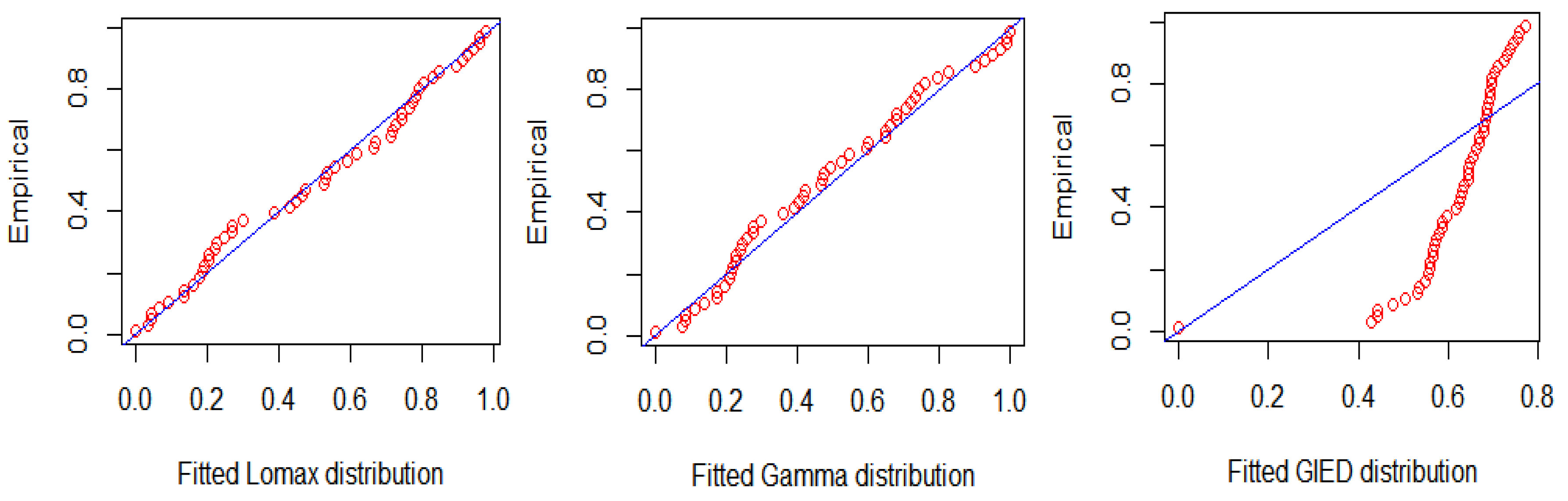
5. Data Analysis
6. Conclusions
Author Contributions
Funding
Acknowledgments
Conflicts of Interest
Appendix A. Likelihood and Log-Likelihood Functions
Appendix B. Lindley Method
References
- Lomax, K.S. Business Failures: Another Example of the Analysis of Failure Data. Publ. Am. Stat. Assoc. 1987, 49, 847–852. [Google Scholar] [CrossRef]
- Ahsanullah, M. Record values of the Lomax distribution. Stat. Neerl. 2010, 45, 21–29. [Google Scholar] [CrossRef]
- Afaq, A.; Ahmad, S.P.; Ahmed, A. Bayesian analysis of shape parameter of Lomax distribution using different loss functions. Int. J. Stat. Math. 2015, 2, 55–65. [Google Scholar]
- Ismail, A.A. Optimum Failure-Censored Step-Stress Life Test Plans for the Lomax Distribution. Strength Mater. 2016, 48, 1–7. [Google Scholar] [CrossRef]
- Lemonte, A.J.; Cordeiro, G.M. An extended Lomax distribution. Statistics 2013, 47, 800–816. [Google Scholar] [CrossRef]
- Cordeiro, G.M.; Ortega, E.M.M.; Popovic, B.V. The gamma-Lomax distribution. J. Stat. Comput. Simul. 2015, 85, 305–319. [Google Scholar] [CrossRef]
- Kilany, N.M. Weighted Lomax distribution. Springerplus 2016, 5, 1862–1880. [Google Scholar] [CrossRef]
- Ahmadi, J.; Crescenzo, A.D.; Longobardi, M. On dynamic mutual information for bivariate lifetimes. Adv. Appl. Probab. 2015, 47, 1157–1174. [Google Scholar] [CrossRef]
- Shannon, C.E. A mathematical theory of communication. Bell Labs Tech. J. 1948, 27, 379–423. [Google Scholar] [CrossRef]
- Cover, T.; Thomas, J. Elements of Information Theory; Wiley: Hoboken, NJ, USA, 2005. [Google Scholar]
- Siamak, N.; Ehsan, S. Shannon entropy as a new measure of aromaticity, Shannon aromaticity. Phys. Chem. Chem. Phys. 2010, 12, 4742–4749. [Google Scholar]
- Tahmasebi, S.; Behboodian, J. Shannon Entropy for the Feller-Pareto (FP) Family and Order Statistics of FP Subfamilies. Appl. Math. Sci. 2010, 4, 495–504. [Google Scholar]
- Cho, Y.; Sun, H.; Lee, K. Estimating the Entropy of a Weibull Distribution under Generalized Progressive Hybrid Censoring. Entropy 2015, 17, 102–122. [Google Scholar] [CrossRef]
- Seo, J.I.; Kang, S.B. Entropy Estimation of Generalized Half-Logistic Distribution (GHLD) Based on Type-II Censored Samples. Entropy 2014, 16, 443–454. [Google Scholar] [CrossRef]
- Epstein, B. Truncated life-tests in the expotential case. Ann. Math. Stat. 1954, 25, 555–564. [Google Scholar] [CrossRef]
- Balakrishnan, N.; Aggarwala, R. Progressive Censoring; Birkhauser: Boston, MA, USA, 2000. [Google Scholar]
- Kundu, D.; Joarder, A. Analysis of Type-II progressively hybrid censored data. Comput. Stat. Data Anal. 2006, 50, 2509–2528. [Google Scholar] [CrossRef]
- Cho, Y.; Sun, H.; Lee, K. An Estimation of the Entropy for a Rayleigh Distribution Based on Doubly-Generalized Type-II Hybrid Censored Samples. Entropy 2014, 16, 3655–3669. [Google Scholar] [CrossRef]
- Kundu, D. On hybrid censored Weibull distribution. J. Stat. Plan. Inference 2007, 137, 2127–2142. [Google Scholar] [CrossRef]
- Ma, Y.; Shi, Y. Inference for Lomax Distribution Based on Type-II Progressively Hybrid Censored Data; Vidyasagar University: Midnapore, India, 2013. [Google Scholar]
- Parsian, A.; Kirmani, S. Handbook of Applied Econometrics and Statistical Inference; Chapter Estimation Under LINEX Loss Function; Marcel Dekker Inc.: New York, NY, USA, 2002; pp. 53–76. [Google Scholar]
- Singh, P.K.; Singh, S.K.; Singh, U. Bayes Estimator of Inverse Gaussian Parameters Under General Entropy Loss Function Using Lindley’s Approximation. Commun. Stat. Simul. Comput. 2008, 37, 1750–1762. [Google Scholar] [CrossRef]
- Lindley, D.V. Approximate Bayesian methods. Trab. Estad. Investig. Oper. 1980, 31, 223–245. [Google Scholar] [CrossRef]
- Tierney, L.; Kadane, J. Accurate Approximations for Posterior Moments and Marginal Densities. Publ. Am. Stat. Assoc. 1986, 81, 82–86. [Google Scholar] [CrossRef]
- Howlader, H.A. Bayesian survival estimation of Pareto distribution of the second kind based on failure-censored data. Comput. Stat. Data Anal. 2002, 38, 301–314. [Google Scholar] [CrossRef]
- Simpson, J. Use of the gamma distribution in single-cloud rainfall analysis. Mon. Weather Rev. 1972, 100, 309–312. [Google Scholar] [CrossRef]
- Giles, D.; Feng, H.; Godwin, R.T. On the bias of the maximum likelihood estimator for the two parameter Lomax distribution. Commun. Stat. Theory Methods 2013, 42, 1934–1950. [Google Scholar] [CrossRef]
- Helu, A.; Samawi, H.; Raqab, M.Z. Estimation on Lomax progressive censoring using the EM algorithm. J. Stat. Comput. Simul. 2015, 85, 1035–1052. [Google Scholar] [CrossRef]


| n | m | k | ||||||||
|---|---|---|---|---|---|---|---|---|---|---|
| h = 0.2 | h = 0.5 | q = 0.2 | q = −0.2 | |||||||
| 60 | 52 | 40 | I | −0.0157 | 0.0518 | 0.0171 | −0.0402 | −0.0712 | −0.0079 | |
| (0.3544) | (0.4323) | (0.4141) | (0.4054) | (0.5412) | (0.4432) | |||||
| 0.0282 | −0.0058 | −0.0566 | −0.0474 | −0.022 | ||||||
| (0.3818) | (0.3706) | (0.3562) | (0.3770) | (0.3766) | ||||||
| II | −0.066 | 0.0331 | 0.0001 | −0.0539 | −0.0619 | −0.0303 | ||||
| (0.374) | (0.4233) | (0.4065) | (0.395) | (0.4669) | (0.4521) | |||||
| −0.0062 | −0.0394 | −0.0912 | −0.0818 | −0.0577 | ||||||
| (0.35) | (0.341) | (0.3329) | (0.3516) | (0.3489) | ||||||
| 48 | I | −0.0265 | 0.1006 | 0.077 | 0.0116 | 0.0433 | 0.0668 | |||
| (0.2412) | (0.4526) | (0.4618) | (0.3594) | (0.5667) | (0.5138) | |||||
| 0.0861 | 0.0633 | 0.0238 | 0.0303 | 0.047 | ||||||
| (0.2981) | (0.2873) | (0.2744) | (0.2871) | (0.2917) | ||||||
| II | −0.0224 | 0.0569 | 0.0312 | −0.0079 | 0.0013 | 0.02 | ||||
| (0.2501) | (0.2706) | (0.2632) | (0.2553) | (0.2662) | (0.2669) | |||||
| 0.0457 | 0.0221 | −0.018 | −0.0135 | 0.0067 | ||||||
| (0.2745) | (0.267) | (0.2574) | (0.2744) | (0.2706) | ||||||
| 100 | 80 | 64 | I | −0.0346 | −0.0692 | −0.0978 | −0.1384 | −0.1935 | −0.1383 | |
| (0.206) | (0.2741) | (0.2948) | (0.3182) | (0.4859) | (0.3755) | |||||
| 0.0319 | 0.0116 | −0.0189 | -0.0129 | 0.0033 | ||||||
| (0.2074) | (0.2025) | (0.1967) | (0.2053) | (0.2056) | ||||||
| II | −0.0601 | −0.025 | −0.046 | −0.077 | −0.081 | −0.0567 | ||||
| (0.2282) | (0.2405) | (0.238) | (0.235) | (0.2712) | (0.2443) | |||||
| 0.0099 | −0.0105 | −0.042 | −0.0361 | −0.0213 | ||||||
| (0.2159) | (0.2115) | (0.2068) | (0.2141) | (0.2147) | ||||||
| 72 | I | −0.031 | 0.0379 | 0.0154 | −0.0125 | −0.0047 | 0.0066 | |||
| (0.1713) | (0.2766) | (0.2481) | (0.2291) | (0.2766) | (0.2538) | |||||
| 0.022 | 0.0062 | −0.0198 | −0.0148 | −0.0026 | ||||||
| (0.1773) | (0.174) | (0.1705) | (0.1763) | (0.1765) | ||||||
| II | −0.0138 | 0.03 | 0.0131 | −0.0128 | −0.0092 | 0.0059 | ||||
| (0.1814) | (0.1914) | (0.1864) | (0.1809) | (0.1944) | (0.1877) | |||||
| 0.0324 | 0.0161 | −0.0105 | −0.0052 | 0.0067 | ||||||
| (0.1805) | (0.1767) | (0.1724) | (0.1779) | (0.1796) | ||||||
| n | m | k | ||||||||
|---|---|---|---|---|---|---|---|---|---|---|
| h = 0.2 | h = 0.5 | q = 0.2 | q = | |||||||
| 60 | 52 | 40 | I | −0.0157 | 0.152 | 0.1181 | 0.0733 | 0.0718 | 0.101 | |
| (0.3544) | (0.3253) | (0.3242) | (0.3577) | (0.3696) | (0.3403) | |||||
| 0.078 | 0.0481 | 0.0005 | 0.0095 | 0.0323 | ||||||
| (0.3025) | (0.2911) | (0.2774) | (0.2936) | (0.2961) | ||||||
| II | −0.066 | 0.0687 | 0.0379 | −0.0173 | −0.0374 | 0.0012 | ||||
| (0.374) | (0.289) | (0.2823) | (0.3057) | (0.4011) | (0.3508) | |||||
| 0.0592 | 0.0294 | −0.0177 | −0.0106 | 0.0139 | ||||||
| (0.2919) | (0.2818) | (0.2703) | (0.284) | (0.2873) | ||||||
| 48 | I | −0.0265 | 0.064 | 0.0391 | 0.0011 | 0.01 | 0.0282 | |||
| (0.2412) | (0.227) | (0.2199) | (0.2122) | (0.2226) | (0.2233) | |||||
| 0.0322 | 0.0091 | −0.0284 | −0.0219 | −0.004 | ||||||
| (0.2242) | (0.2184) | (0.2125) | (0.2225) | (0.2233) | ||||||
| II | −0.0224 | 0.0692 | 0.0437 | 0.0048 | 0.0116 | 0.03 | ||||
| (0.2501) | (0.2307) | (0.2223) | (0.2129) | (0.2312) | (0.2331) | |||||
| 0.0338 | 0.0109 | −0.0268 | −0.0213 | −0.0032 | ||||||
| (0.2408) | (0.2352) | (0.2289) | (0.2399) | (0.2394) | ||||||
| 100 | 80 | 64 | I | −0.0346 | 0.0229 | −0.0009 | −0.0309 | −0.0393 | −0.016 | |
| (0.206) | (0.1948) | (0.2015) | (0.1963) | (0.2426) | (0.2195) | |||||
| 0.0563 | 0.0371 | 0.0073 | 0.0133 | 0.0278 | ||||||
| (0.1748) | (0.1702) | (0.1644) | (0.1709) | (0.1716) | ||||||
| II | −0.0601 | 0.0254 | 0.0052 | −0.0256 | −0.0186 | −0.0037 | ||||
| (0.2282) | (0.2015) | (0.1965) | (0.1912) | (0.1986) | (0.1989) | |||||
| 0.0488 | 0.0295 | −0.0007 | 0.0048 | 0.0197 | ||||||
| (0.1989) | (0.1942) | (0.188) | (0.1954) | (0.1966) | ||||||
| 72 | I | −0.031 | 0.0289 | 0.012 | −0.0137 | −0.0077 | 0.0046 | |||
| (0.1713) | (0.16) | (0.1568) | (0.1534) | (0.1585) | (0.1586) | |||||
| 0.0426 | 0.0269 | 0.0013 | 0.006 | 0.0183 | ||||||
| (0.1649) | (0.1614) | (0.1573) | (0.1623) | (0.1631) | ||||||
| II | −0.0138 | 0.0484 | 0.0316 | 0.0058 | 0.012 | 0.0244 | ||||
| (0.1814) | (0.172) | (0.1659) | (0.1599) | (0.1659) | (0.1671) | |||||
| 0.0395 | 0.0231 | −0.0026 | 0.0018 | 0.0149 | ||||||
| (0.1573) | (0.154) | (0.1502) | (0.1556) | (0.1552) | ||||||
| No. | Distribution | K-S | p Value | |||
|---|---|---|---|---|---|---|
| 1. | Lomax distribution | 681.4757 | 685.3782 | 0.0952 | 0.7337 | |
| 2. | Gamma distribution | 682.1883 | 686.0908 | 0.0893 | 0.8009 | |
| 3. | Generalized inverted exponential distribution | 788.2046 | 792.1071 | 0.4184 |
| h = 0.2 | h = 0.5 | q = 0.2 | q = | ||||
|---|---|---|---|---|---|---|---|
| I | 7.514680 | 7.391941 | 7.199010 | 6.966619 | 7.236140 | 7.286647 | Lindley |
| 8.047029 | 7.699564 | 7.452938 | 7.731689 | 8.073602 | TK | ||
| II | 6.595185 | 6.167338 | 6.102223 | 6.029770 | 6.108076 | 6.126530 | Lindley |
| 6.975125 | 6.821545 | 6.717372 | 6.856352 | 6.883334 | TK | ||
| III | 6.956195 | 6.586184 | 6.462234 | 6.324426 | 6.478268 | 6.512196 | Lindley |
| 7.462613 | 7.187117 | 7.023052 | 7.259597 | 7.390569 | TK | ||
© 2019 by the authors. Licensee MDPI, Basel, Switzerland. This article is an open access article distributed under the terms and conditions of the Creative Commons Attribution (CC BY) license (http://creativecommons.org/licenses/by/4.0/).
Share and Cite
Liu, S.; Gui, W. Estimating the Entropy for Lomax Distribution Based on Generalized Progressively Hybrid Censoring. Symmetry 2019, 11, 1219. https://doi.org/10.3390/sym11101219
Liu S, Gui W. Estimating the Entropy for Lomax Distribution Based on Generalized Progressively Hybrid Censoring. Symmetry. 2019; 11(10):1219. https://doi.org/10.3390/sym11101219
Chicago/Turabian StyleLiu, Shuhan, and Wenhao Gui. 2019. "Estimating the Entropy for Lomax Distribution Based on Generalized Progressively Hybrid Censoring" Symmetry 11, no. 10: 1219. https://doi.org/10.3390/sym11101219
APA StyleLiu, S., & Gui, W. (2019). Estimating the Entropy for Lomax Distribution Based on Generalized Progressively Hybrid Censoring. Symmetry, 11(10), 1219. https://doi.org/10.3390/sym11101219