A Sparsity-Aware Variable Kernel Width Proportionate Affine Projection Algorithm for Identifying Sparse Systems

Abstract

A sparsity-aware variable kernel width proportionate affine projection (AP) algorithm is devised for identifying sparse system in impulsive noise environments. For the devised algorithm, the symmetry maximum correntropy criterion (MCC) is employed to develop a new cost function for improving the PAP algorithm, then the variable kernel width and the $l_p$-norm-like constraint are incorporated into the cost-function, which is named as $l_p$-norm variable kernel width proportionate affine projection (LP-VPAP) algorithm. The devised LP-VPAP algorithm is investigated and verified under impulsive interference environments. Experimental results show that the LP-VPAP gets a faster convergence and provides a lower steady-state performance compared with AP, zero-attracting AP (ZA-AP), reweighted ZA-AP (RZA-AP), proportionate AP (PAP), MCC, variable kernel width MCC (VKW-MCC), and proportionate AP MCC (PAPMCC) algorithms.

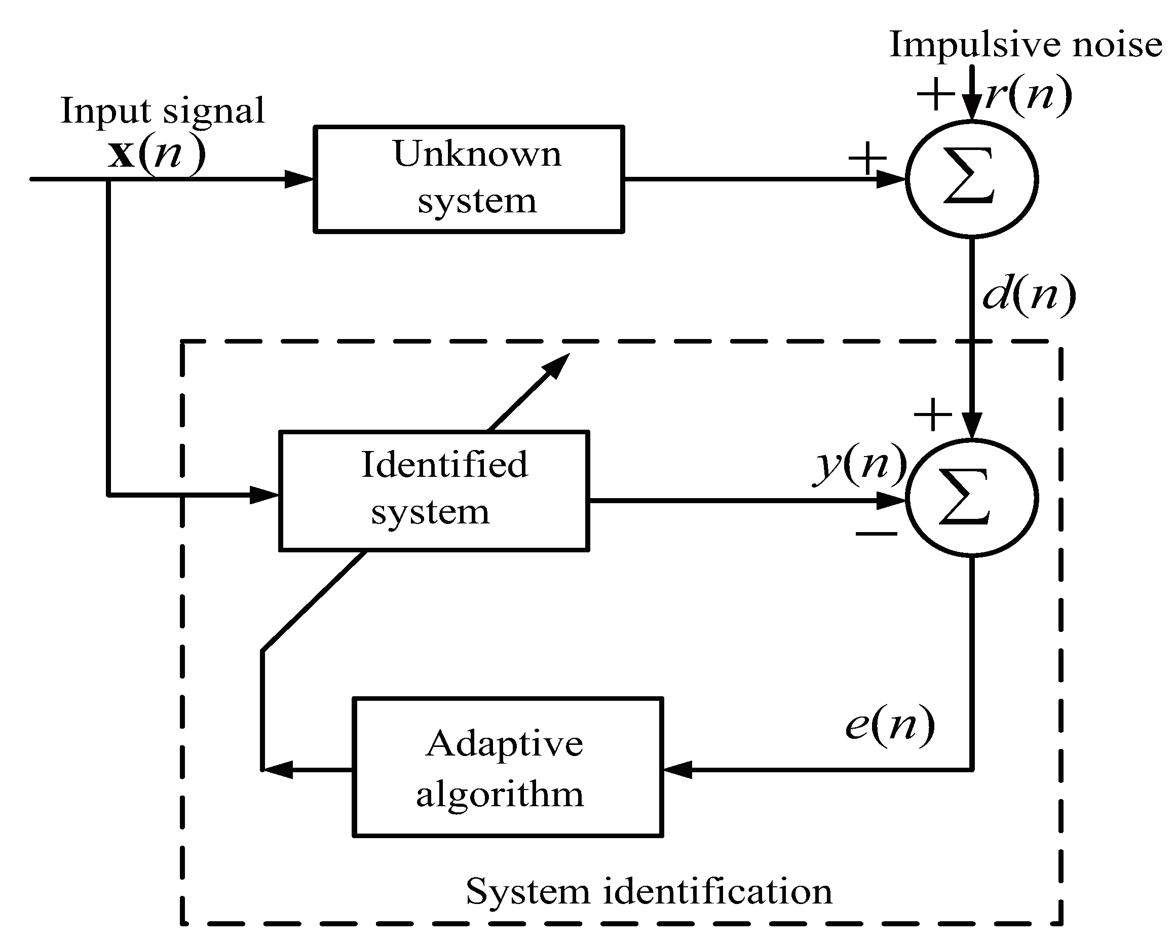
1. Introduction

Today, with the evolution of information technology, adaptive filtering (AF) algorithms are used in wireless communication, noise reduction, system identification (SI), and automatic control systems [1,2,3,4,5,6]. The famed least-mean-square (LMS) is one of the classic algorithms and is generally used [7,8]. Then, the normalized version of the LMS (NLMS) is proposed to improve the stability as well as increase the convergence performance [9]. However, the LMS-like algorithms encounter poor performance while the input is a strongly correlated signal. On the basis of the NLMS, the affine projection (AP) is developed by reusing input signal [10,11], which is regarded as a multi-order generalization of the NLMS algorithm, reusing the sample values of the current time and the previous time of the input signal. Compared with the LMS and NLMS, the behavior of the AP algorithms is more outstanding, especially for the colored inputs [12].

Recently, scholars have found that sparse systems are widespread in nature [13,14,15,16,17,18]. For example, in underwater communication systems, the underwater acoustic channel exhibits strong sparsity [19]. In network communications, the network echo channel also exhibits sparsity. [20]. However, the traditional LMS, NLMS and AP algorithms show great potential that can be further improved to use the sparse characteristic in the system’s impulse response (IR). To fully use the sparse characteristic, the literature [21] has proposed the famed proportionate NLMS (PNLMS) algorithm by introducing a proportionate update technique to reasonably allocate the step sizes corresponding to each filter tap coefficient. Inspired by the PNLMS, the proportionate AP (PAP) algorithm was proposed by using the idea in PNLMS to fully use the sparsity in the system via employing the data reusing principle [22]. Then, various proportionate-type AF algorithms were proposed and analyzed [23,24,25]. Moreover, a collection of zero-attraction (ZA) algorithms, such as the ZA-LMS and its reweighted form (RZA-LMS), ZA-AP, and RZA-AP algorithms, etc. [26,27,28,29,30,31,32,33], are developed based on the concept of compressed sensing (CS) theory [34] for sparse SI.

In many engineering fields, noise often exhibits strongly impulsive characteristics [35]. Traditional LMS-type and AP-type algorithms, which use the $E\left\{e^2\left(n\right)\right\}$ (where $e\left(n\right)$ is the error signal, and $E\left\{·\right\}$ represents the expectation operator) to construct an expected cost-function, will encounter poor performance in impulsive noise environments. To find out the solution for handling these problems, the maximum correntropy criterion (MCC) was proposed to give resistance to impulse-noise [36,37]. Then, a series of AF algorithms based on MCC were proposed to resist impulse-noise [38,39,40,41,42,43,44,45,46,47,48]. The variable kernel width MCC (VKW-MCC) uses a variable kernel width technique to enhance the identification ability of the famed MCC [49]. The proportionate affine projection symmetry maximum correntropy criterion (PAPMCC) uses the MCC and the data reusing technique to enhance the robustness of the PAP [50].

The MCC criterion is used in this paper to build a new cost function to improve PAP algorithm, then integrate the variable kernel width technique and the $l_p$-norm-like constraint into the cost-function to develop the $l_p$-norm variable kernel width proportionate affine projection (LP-VPAP). The devised LP-VPAP algorithm is investigated and verified under impulsive noise environments. Experimental results show that the LP-VPAP converges the fastest and gets the lowest steady state misalignment compared with AP, ZA-AP, RZA-AP, PAP, MCC, VKW-MCC, and PAPMCC algorithms.

2. Previous Work of the MCC and AP Algorithms

2.1. The Basic MCC Algorithm

In the range of AF, the implementation schematic diagram for SI is presented in Figure 1.

$\mathbf{x}\left(n\right)=\left[x\right(n),x(n-1),\cdots ,$$x(n-L+1){]}^T$ is used as system input signal, and the IR is modeled as $\mathbf{h}\left(n\right)={\left[h_0\left(n\right),\cdots ,h_{\mathrm{L}-1}\left(n\right)\right]}^T$ with L elements, and n represents the time index. The achieved signal $d\left(n\right)$ is

$$d\left(n\right)={\mathbf{x}}^T\left(n\right)\mathbf{h}\left(n\right)+r\left(n\right),$$

(1)

in which $r\left(n\right)$ denotes the additive interferences. The output signal is defined as

$$y\left(n\right)={\mathbf{x}}^T\left(n\right)\widehat{\mathbf{h}}\left(n\right),$$

(2)

in which $\widehat{\mathbf{h}}\left(n\right)$ stands for the estimation vector of IR. $e\left(n\right)$ is the estimated error written as

$$e\left(n\right)=d\left(n\right)-y\left(n\right).$$

(3)

The famed MCC aims to solve the following cost-function

$$J_{\mathrm{MCC}}\left(n\right)=E\left[exp\left(-\frac{e^2\left(n\right)}{2{\sigma }^2}\right)\right],$$

(4)

where $\sigma$ represents Gaussian kernel. Removing expectation operator and computing the gradient of Equation (4), the iterative formula of the MCC is

$$\widehat{\mathbf{h}}(n+1)=\widehat{\mathbf{h}}\left(n\right)+{\mu }_{\mathrm{MCC}}exp(-\frac{e^2\left(n\right)}{2{\sigma }^2})e\left(n\right)\mathbf{x}\left(n\right),$$

(5)

in which ${\mu }_{\mathrm{MCC}}$ is the step size.

2.2. AP Algorithm

The AP algorithm reuses the information from previous instants to accelerate the convergence, particularly for colored input. The input data of the AP is expressed as an $L\times P$ matrix

$$\mathbf{X}\left(n\right)=\left[\mathbf{x}\right(n),\mathbf{x}(n-1),\mathbf{x}(n-2),\cdots ,\mathbf{x}(n-P+1\left)\right].$$

(6)

Herein, P denotes the order of the projection. The reference signal in the AP algorithm is $\mathbf{d}\left(n\right)={[d\left(n\right),d(n-1),d(n-2),\cdots ,d(n-P+1)]}^{\mathrm{T}}$. Then, the output is

$$\mathbf{y}\left(n\right)={\mathbf{X}}^T\left(n\right)\widehat{\mathbf{h}}\left(n\right)$$

(7)

with the error vector

$$\mathbf{e}\left(n\right)=\mathbf{d}\left(n\right)-\mathbf{y}\left(n\right).$$

(8)

The iterative formula of the famous AP is denoted as

$$\widehat{\mathbf{h}}\left(n\right)=\widehat{\mathbf{h}}(n-1)+{\mu }_{\mathrm{AP}}\mathbf{X}\left(n\right){\left[{\mathbf{X}}^T\left(n\right)\mathbf{X}\left(n\right)+{\delta }_{\mathrm{AP}}{\mathbf{I}}_P\right]}^{-1}\mathbf{e}\left(n\right),$$

(9)

in which ${\mu }_{\mathrm{AP}}$ represents the total step size, ${\delta }_{\mathrm{AP}}>0$ has a small value, and ${\mathbf{I}}_P$ is a $P\times P$ identity matrix.

3. The Developed LP-VPAP Algorithm

Herein, we detailedly analyze the developed LP-VPAP algorithm, which is implemented by the variable kernel width technique and the $l_p$-norm-like constraint to devise a novel cost-function. In addition, it can be summarized as the following problem:

$$\begin{array}{c}{\displaystyle \frac{1}{2}{∥\widehat{\mathbf{h}}(n+1)-\widehat{\mathbf{h}}\left(n\right)∥}_{{\mathbf{K}}^{-1}\left(n\right)}^2+\rho {∥{\mathbf{K}}^{-1}\left(n\right)\widehat{\mathbf{h}}(n+1)∥}_p^p}\hfill \\ {\displaystyle \mathrm{subject}\mathrm{to}\stackrel{⌣}{\mathbf{e}}}\left(n\right)=\left[{\mathbf{1}}_P-\xi exp\left(-\frac{\mathbf{e}\left(n\right)\odot \mathbf{e}\left(n\right)}{2{\sigma }^2}\right)\right]\odot \mathbf{e}\left(n\right)\hfill \end{array}$$

(10)

where $\stackrel{⌣}{\mathbf{e}}$(n) = d(n) − X^T(n)$\widehat{\mathbf{h}}$(n + 1), ${∥\widehat{\mathbf{h}}(n+1)∥}_p^p=\sum _{i=0}^L{\left|h_i\right|}^p$, 1_P is a P × 1 vector with all the elements equal to 1, ξ denotes the step size, and e(n) ⊙ e(n) is the Hadamard product. K(n) s a gain assignment matrix which allots different gain to each coefficient [21]:

$$\mathbf{K}\left(n\right)=\mathrm{diag}\left\{\left.k_0\left(n\right),k_1\left(n\right),\dots ,k_{L-1}\left(n\right)\right\}\right..$$

(11)

The individual gain $k_l\left(n\right)$ is

$$k_l\left(n\right)=\frac{{\phi }_l\left(n\right)}{{\displaystyle \sum _{i=0}^{L-1}}{\phi }_i(n-1)},$$

(12)

with

$$\begin{array}{c}{\phi }_l(n-1)=max\left\{\alpha q,\left|{\widehat{h}}_l\right|\right\},\hfill \\ q=max\left\{\beta ,\left|{\widehat{h}}_0\right|,\left|{\widehat{h}}_1\right|,\left|{\widehat{h}}_2\right|,\cdots ,\left|{\widehat{h}}_{L-1}\right|\right\}.\hfill \end{array}$$

(13)

Parameters $\alpha$ and $\beta$ can maintain coefficient updating from halting. Employing the Lagrange multiplier (LM) method, the cost-function of the developed LP-VPAP is

$$\begin{array}{c}{\displaystyle J\left(\widehat{\mathbf{h}}(n+1)\right)=\frac{1}{2}{∥\widehat{\mathbf{h}}(n+1)-\widehat{\mathbf{h}}\left(n\right)∥}_{{\mathbf{K}}^{-1}\left(n\right)}^2+\rho {∥{\mathbf{K}}^{-1}\left(n\right)\widehat{\mathbf{h}}(n+1)∥}_p^p}\hfill \\ {\displaystyle +\mathbf{\lambda }\left\{\stackrel{⌣}{\mathbf{e}}\left(n\right)-\left[{\mathbf{1}}_P-\xi exp\left(-\frac{\mathbf{e}\left(n\right)\odot \mathbf{e}\left(n\right)}{2{\sigma }^2}\right)\right]\odot \mathbf{e}\left(n\right)\right\}}\hfill \end{array}$$

(14)

in which $\mathit{\lambda }=[{\lambda }_0,{\lambda }_1,\dots ,{\lambda }_{\mathrm{P}-1}]$. Then, the gradients of $J\left(\widehat{\mathbf{h}}(n+1)\right)$ with respect to $\widehat{\mathbf{h}}(n+1)$ and $\mathit{\lambda }$ are calculated, respectively.

$$\frac{\partial J\left(\widehat{\mathbf{h}}(n+1)\right)}{\partial \widehat{\mathbf{h}}(n+1)}={\mathbf{K}}^{-1}\left(n\right)\left(\widehat{\mathbf{h}}(n+1)-\widehat{\mathbf{h}}\left(n\right)\right)+\rho \frac{p{\mathbf{K}}^{-1}\left(n\right)\mathrm{sgn}\left(\widehat{\mathbf{h}}(n+1)\right)}{\epsilon +{\left|\widehat{\mathbf{h}}(n+1)\right|}^{1-p}}-\mathbf{X}\left(n\right){\mathit{\lambda }}^T$$

(15)

and

$$\frac{\partial J\left(\widehat{\mathbf{h}}(n+1)\right)}{\partial \mathit{\lambda }}=\stackrel{⌣}{\mathbf{e}}\left(n\right)-\left[{\mathbf{1}}_P-\xi exp\left(-\frac{\mathbf{e}\left(n\right)\odot \mathbf{e}\left(n\right)}{2{\sigma }^2}\right)\right]\odot \mathbf{e}\left(n\right).$$

(16)

Assume that $\widehat{\mathbf{h}}(n+1)\approx \widehat{\mathbf{h}}\left(n\right)$ and let

$$\begin{array}{c}{\displaystyle \frac{\partial J\left(\widehat{\mathbf{h}}(n+1)\right)}{\partial \widehat{\mathbf{h}}(n+1)}=\mathbf{0}}\hfill \\ {\displaystyle \frac{\partial J\left(\widehat{\mathbf{h}}(n+1)\right)}{\partial \mathit{\lambda }}=\mathbf{0}.}\hfill \end{array}$$

(17)

Then, one can obtain

$$\widehat{\mathbf{h}}(n+1)=\widehat{\mathbf{h}}\left(n\right)+\mathbf{K}\left(n\right)\mathbf{X}\left(n\right){\mathit{\lambda }}^T-\rho \frac{p\mathrm{sgn}\left(\widehat{\mathbf{h}}\left(n\right)\right)}{\epsilon +{\left|\widehat{\mathbf{h}}\left(n\right)\right|}^{1-p}},$$

(18)

where $\epsilon$ is a small positive constant which aims to prevent division by 0 and

$$\mathbf{d}\left(n\right)={\mathbf{X}}^T\left(n\right)\widehat{\mathbf{h}}(n+1)+\left[{\mathbf{1}}_P-\xi exp\left(-\frac{\mathbf{e}\left(n\right)\odot \mathbf{e}\left(n\right)}{2{\sigma }^2}\right)\right]\odot \mathbf{e}\left(n\right).$$

(19)

From Equations (18) and (19), we have

$${\mathit{\lambda }}^T=\xi {\left[{\mathbf{X}}^T\left(n\right)\mathbf{K}\left(n\right)\mathbf{X}\left(n\right)\right]}^{-1}exp\left(-\frac{\mathbf{e}\left(n\right)\odot \mathbf{e}\left(n\right)}{2{\sigma }^2}\right)\odot \mathbf{e}\left(n\right)+\rho {\left[{\mathbf{X}}^T\left(n\right)\mathbf{K}\left(n\right)\mathbf{X}\left(n\right)\right]}^{-1}{\mathbf{X}}^T\left(n\right)\frac{p\mathrm{sgn}\left(\widehat{\mathbf{h}}\left(n\right)\right)}{\epsilon +{\left|\widehat{\mathbf{h}}\left(n\right)\right|}^{1-p}}$$

(20)

Then, the iterative formula is denoted as

$$\begin{array}{c}{\displaystyle \widehat{\mathbf{h}}(n+1)=\widehat{\mathbf{h}}\left(n\right)+\xi \mathbf{K}\left(n\right)\mathbf{X}\left(n\right){\left[{\mathbf{X}}^T\left(n\right)\mathbf{K}\left(n\right)\mathbf{X}\left(n\right)\right]}^{-1}exp\left(-\frac{\mathbf{e}\left(n\right)\odot \mathbf{e}\left(n\right)}{2{\sigma }^2}\right)\odot \mathbf{e}\left(n\right)}\hfill \\ {\displaystyle +\rho \mathbf{K}\left(n\right)\mathbf{X}\left(n\right){\left[{\mathbf{X}}^T\left(n\right)\mathbf{K}\left(n\right)\mathbf{X}\left(n\right)\right]}^{-1}{\mathbf{X}}^T\left(n\right)\frac{p\mathrm{sgn}\left(\widehat{\mathbf{h}}\left(n\right)\right)}{\epsilon +{\left|\widehat{\mathbf{h}}\left(n\right)\right|}^{1-p}}-\rho \frac{p\mathrm{sgn}\left(\widehat{\mathbf{h}}\left(n\right)\right)}{\epsilon +{\left|\widehat{\mathbf{h}}\left(n\right)\right|}^{1-p}}}\hfill \end{array}$$

(21)

In practice, the third term in Equation (21) plays a minor role and hence it can be ignored here [51,52]. To enhance the behavior of correntropy-based algorithm, a variable kernel width technique is used to automatically adjust the $\sigma$ in Equation (4). Suppose that there is no impulse-interference. After obtaining $e\left(n\right)$, the kernel-width which yields the error with the maximum damping along the direction of gradient-ascent is solved by

$$\underset{\sigma \left(n\right)}{max}{J}_{\mathrm{MCC}}\left(n\right)=exp\left(-\frac{e^2\left(n\right)}{2{\sigma }^2\left(n\right)}\right).$$

(22)

For Equation (22), calculate its derivative in terms of $e\left(n\right)$, then let the derivative be zero, we obtain

$$\sigma \left(n\right)=e\left(n\right){\sigma }^{\prime }\left(n\right).$$

(23)

Solving homogeneous differential Equation (23), we can get

$$\sigma \left(n\right)=\theta \left|e\left(n\right)\right|.$$

(24)

$\sigma \left(n\right)$ represents the optimal kernel-width, and $\theta$ denotes a positive constant. In practical terms, the received signal could contain impulse-interferences. To get the robustness, a observed sliding window of $e\left(n\right)$ is used to optimize $\sigma \left(n\right)$.

$$\sigma \left(n\right)=min({\sigma }_0,\theta \overline{e}\left(n\right)),$$

(25)

in which ${\sigma }_0$ represents a kernel bound, and $\overline{e}\left(n\right)$ is denoted as

$$\overline{e}\left(n\right)=\chi \overline{e}(n-1)+(1-\chi )min\left[e\left(n\right),e(n-1),\cdots ,e(n-N_0+1)\right],$$

(26)

in which $0\ll \chi <1$ denotes a forgetting factor, and $N_0$ represents the observation length. Then, Equation (21) is changed to be

$$\begin{array}{c}{\displaystyle \widehat{\mathbf{h}}(n+1)=\widehat{\mathbf{h}}\left(n\right)+\xi \mathbf{K}\left(n\right)\mathbf{X}\left(n\right){\left[{\mathbf{X}}^T\left(n\right)\mathbf{K}\left(n\right)\mathbf{X}\left(n\right)+{\delta }_{\mathrm{PAP}}{\mathbf{I}}_P\right]}^{-1}exp\left(-\frac{\mathbf{e}\left(n\right)\odot \mathbf{e}\left(n\right)}{2{\sigma }^2\left(n\right)}\right)\odot \mathbf{e}\left(n\right)}\hfill \\ {\displaystyle -\rho \frac{p\mathrm{sgn}\left(\widehat{\mathbf{h}}\left(n\right)\right)}{\epsilon +{\left|\widehat{\mathbf{h}}\left(n\right)\right|}^{1-p}}}\hfill \end{array}$$

(27)

Equation (27) is the final iterative formula for the developed LP-VPAP algorithm.

The computation complexity of the LP-VPAP is compared with MCC, VKW-MCC, AP, ZA-AP, RZA-AP, PAP, and PAPMCC algorithms with respect to the total number of addition, multiplication, and division in each iteration. The comparison is presented in

Table 1. Computational Complexity in Each Iteration.

Algorithm	Addition	Multiplication	Division
MCC	$2L$	$2L+5$	1
VKW-MCC	$2L+2$	$2L+8$	1
AP	$(2P^2+P)L$	$(2P^2+3P)L+P^2$	0
ZA-AP	$(2P^2+P+1)L$	$(2P^2+3P+1)L+P^2$	0
RZA-AP	$(2P^2+P+2)L$	$(2P^2+3P+2)L+P^2$	L
PAP	$2P{L}^2+(2P^2-P+1)L-1$	$2P{L}^2+(2P^2+3P+1)L+P^2$	L
PAPMCC	$2P{L}^2+(2P^2-P+1)L-1$	$2P{L}^2+(2P^2+3P+1)L+P^2+2P$	$L+P$
LP-VPAP	$2P{L}^2+(2P^2-P+3)L+1$	$2P{L}^2+(2P^2+3P+2)L+P^2+2P+4$	$2L+P$

. It is clear to see that the LP-VPAP algorithm has a modest increase in computational complexity compared with that of the PAPMCC algorithm.

4. Performance Analysis

Herein, several examples are presented to investigate the performance of the devised LP-VPAP with the framework of SI. The background noise $r\left(n\right)$ consists of the impulsive noise $i\left(n\right)$ and white-Gaussian-noise (WGN) $v\left(n\right)$, where $i\left(n\right)$ is modeled by the Bernoulli distribution for $i\left(n\right)=b\left(n\right)g\left(n\right)$, $g\left(n\right)$ is another WGN and $b\left(n\right)$ is Bernoulli-process for $P\left(b\right(n)=1)=0.1$. The signal-noise-ratio (SNR) and signal-interface-ratio (SIR), which are defined by $\mathrm{SNR}=10{log}_{10}\frac{{\delta }_x^2}{{\delta }_v^2}$ and $\mathrm{SIR}=10{log}_{10}\frac{{\delta }_x^2}{{\delta }_i^2}$ (where ${\delta }_x^2$, ${\delta }_v^2$, and ${\delta }_i^2$ represent the variances of $x\left(n\right)$, $v\left(n\right)$, and $i\left(n\right)$, respectively), are set as 30 dB and 10 dB, respectively. In all experiments, $L=1024$ and $P=4$ are selected. Regularization parameters are set to be ${\delta }_{\mathrm{AP}}={\delta }_{\mathrm{ZA}-\mathrm{AP}}={\delta }_{\mathrm{RZA}-\mathrm{AP}}$ and ${\delta }_{\mathrm{LP}-\mathrm{VPAP}}={\delta }_{\mathrm{PAP}}=\frac{1}{L}{\delta }_{\mathrm{AP}}$ [53]. The kernel width of the MCC is set as 1, and the observation length of VKW-MCC and LP-VPAP algorithms is set to be 25. The network echo channel used for the simulation, which is a classical sparse channel presented in Figure 2, whose active coefficients distributed in [257,272], is considered to evaluate the proposed LP-VPAP. The behavior of the LP-VPAP is evaluated by normalized-misalignment (NM) that has a definition of $10{log}_{10}({∥\mathbf{h}-\widehat{\mathbf{h}}∥}_2^2/{∥\mathbf{h}∥}_2^2)$.

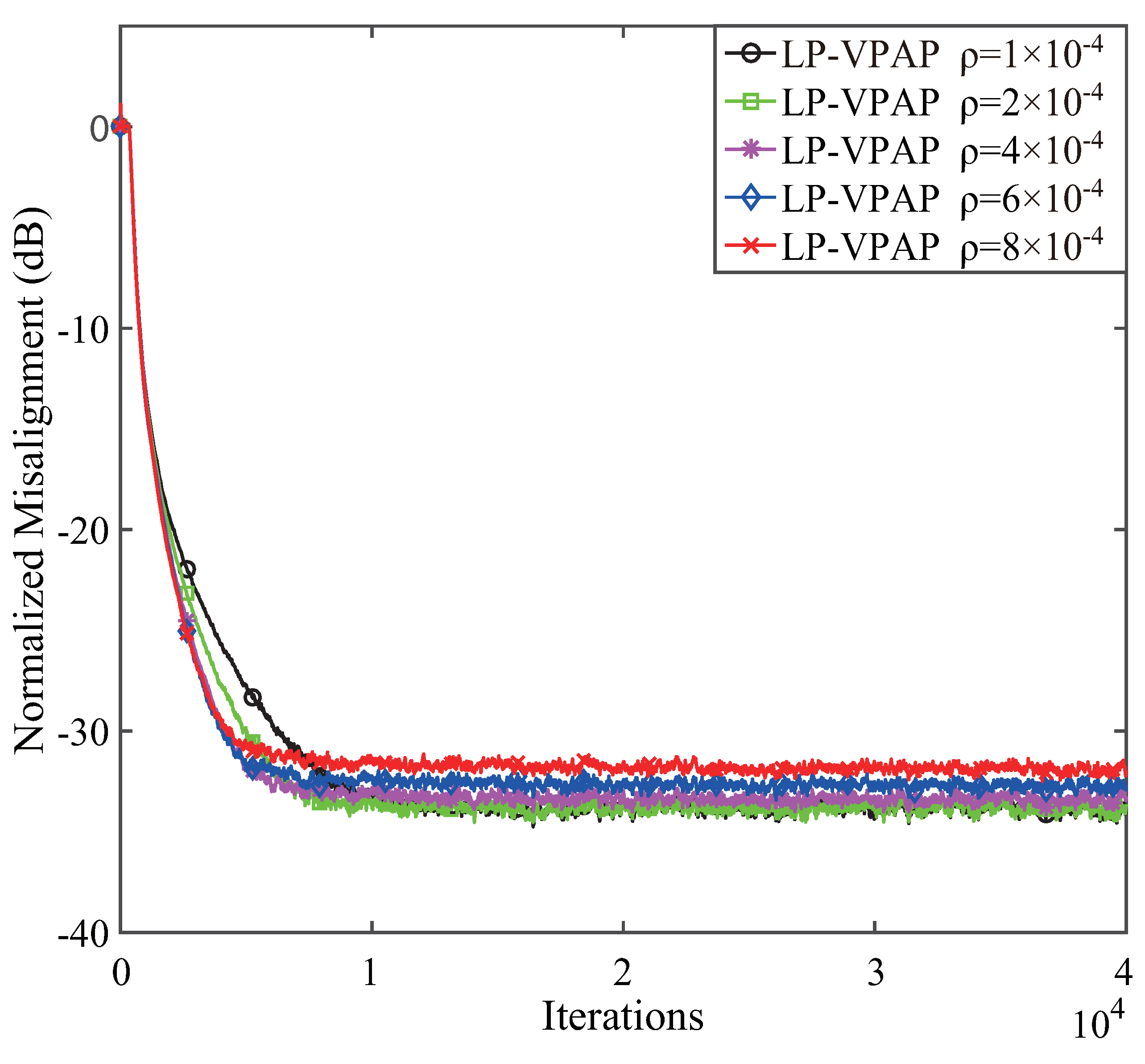
4.1. Performance of the LP-VPAP with Different p and $\rho$

Firstly, the effects of p and $\rho$ on the behavior for devised LP-VPAP algorithm is investigated. The colored noise (CN), which is obtained from WGN filtering through an autoregressive with a pole at 0.8, is used as the input. Herein, $\xi =0.225$. The results given in Figure 3 illustrate that when p is selected to 0.5 or 0.3, the LP-VPAP algorithm achieves the fastest convergence.

Secondly, the effects of $\rho$ on the convergence for the LP-VPAP is analyzed and discussed. Herein, $p=0.5$ is selected. The results given in Figure 4 illustrate that the NM of the LP-VPAP algorithm increases with the increment of $\rho$, but the convergence rate becomes faster. Therefore, a balance between convergence and NM should be taken into consideration.

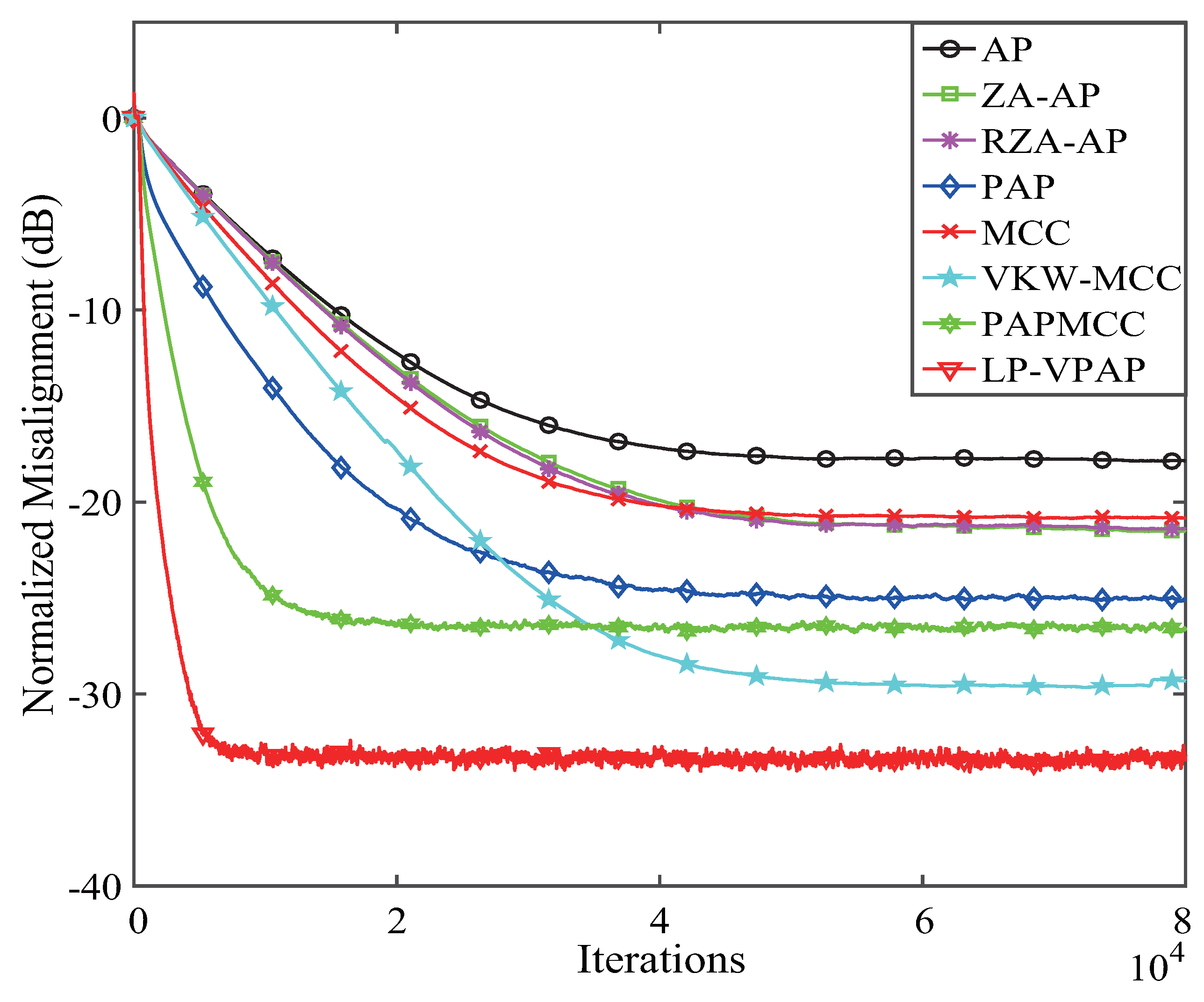
4.2. Performance Comparisons of the LP-VPAP Algorithm under Different Input Signals

According to the simulation above, we found that the devised LP-VPAP obtains better performance when $p=0.5$ and $\rho =4\times {10}^{-7}$ are selected. Then, the identification behavior of the LP-VPAP is compared with AP, ZA-AP, RZA-AP, PAP, MCC, VKW-MCC, and PAPMCC algorithms with WGN and CN input. The step-sizes for other algorithms are presented as follows: ${\mu }_{\mathrm{AP}}={\mu }_{\mathrm{ZA}-\mathrm{AP}}={\mu }_{\mathrm{RZA}-\mathrm{AP}}=0.025$, ${\mu }_{\mathrm{PAP}}=0.005$, ${\mu }_{\mathrm{MCC}}=0.0006$, ${\mu }_{\mathrm{VKW}-\mathrm{MCC}}=0.00175$, and ${\mu }_{\mathrm{PAPMCC}}=0.015$. The performance comparisons of the LP-VPAP with various inputs are presented in Figure 5 and Figure 6, respectively. It is clear to see that the LP-VPAP algorithm achieves the lowest NM and fast convergence rate. When the input is CN, the convergence speed of the MCC and VKW-MCC becomes much slower, while the proposed LP-VPAP is still better than all the related algorithms by considering the convergence and identification error.

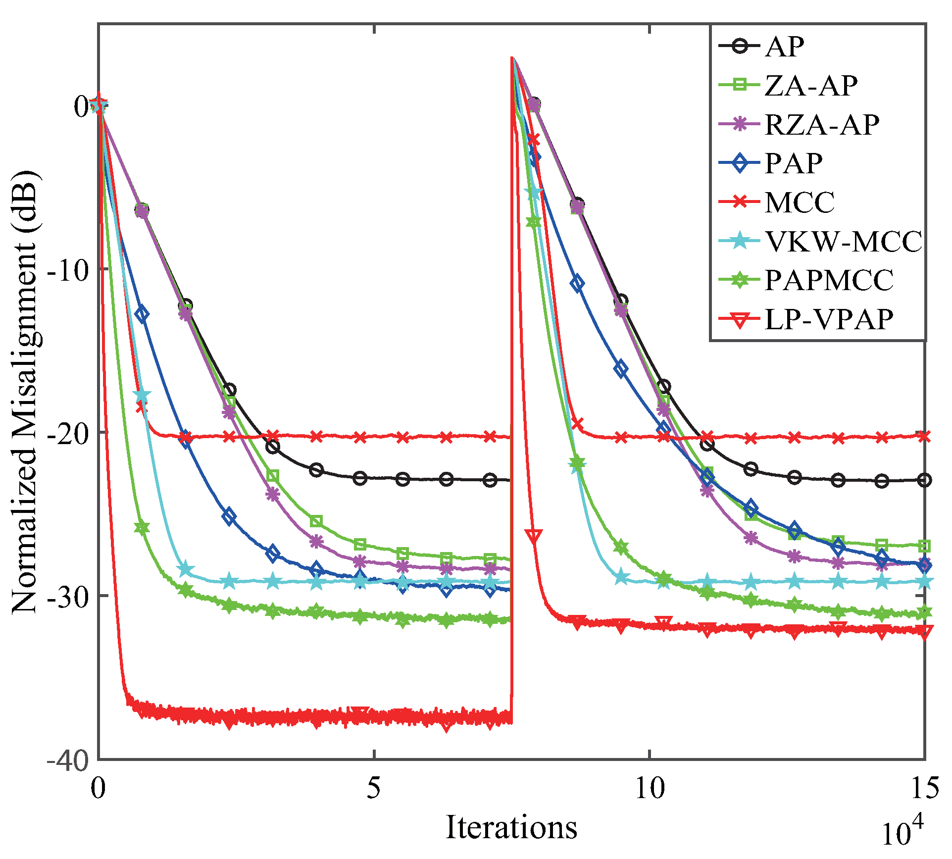
4.3. Tracking Behavior of the LP-VPAP

Herein, the tracking behavior of the LP-VPAP is investigated by two different systems. The first system, whose dominant taps distributed in [257,272], is presented in Figure 7a, and the second system, whose dominant taps distributed in [769,784] and [257,272], is presented in Figure 7b. Other parameters are consistent with those in the previous subsection. Simulation results under different input signal are presented in Figure 8 and Figure 9. It is clear to see that the LP-VPAP tracks the two different sparse systems, and converges the fastest and achieves the lowest NM. In the comparisons, only the sparsity-aware algorithms like ZA-AP, RZA-AP, PAPMCC and the proposed LP-VPAP algorithms will lead to estimation error increase. In Figure 8 and Figure 9, we find this result since our proposed LP-VPAP algorithm is also a sparsity-aware algorithm. Thus, when the system is getting less sparse, our proposed LP-VPAP algorithm will result in a high estimation error like the ZA-AP, RZA-AP and PAPMCC algorithms. However, the LP-VPAP algorithm still provides the lowest estimation error.

4.4. Performance Comparisons of the LP-VPAP Algorithm with a Less Sparse Echo Path

In this subsection, the performance of the LP-VPAP is investigated using CN input with a less sparse echo path whose dominant taps are distributed in [257,384]. Herein, $\rho =5\times {10}^{-8}$ is selected. Other parameters are the same as those in the previous simulations. Simulation results are presented in Figure 10. It is clear to see that although the steady-state error of the devised LP-VPAP increases, it is still better than the related algorithms for providing the fastest convergence speed.

5. Conclusions

In this paper, a sparsity-aware variable kernel width PAP is devised for sparse SI under impulsive noise environments. The developed LP-VPAP is realized by developing the variable kernel width technique and the $l_p$-norm-like constraint. The key parameters are analyzed to discuss the performance of the developed LP-VPAP. Simulation results show the LP-VPAP can speed up the convergence and improve the estimation accuracy compared with AP, ZA-AP, RZA-AP, PAP, MCC, VKW-MCC, and PAPMCC algorithms.

References

- Ljung, L. System Identification: Theory for the User; Prentice-Hall: Upper Saddle River, NJ, USA, 1987. [Google Scholar]
- Benesty, J.; Gänsler, T.; Morgan, D.R.; Sondhi, M.M.; Gay, S.L. Advances in Network and Acoustic Echo Cancellation; Springer: Berlin, Germany, 2001. [Google Scholar]
- Li, Y.; Wang, Y.; Jiang, T. Sparse-aware set-membership NLMS algorithms and their application for sparse channel estimation and echo cancelation. AEU-Int. J. Electron. Commun. 2006, 70, 895–902. [Google Scholar] [CrossRef]
- Li, Y.; Wang, Y.; Yang, R.; Ablu, F. A soft parameter function penalized normalized maximum correntropy criterion algorithm for sparse system identification. Entropy 2017, 19, 45. [Google Scholar] [CrossRef]
- Li, Y.; Wang, Y.; Jiang, T. Norm-adaption penalized least mean square/fourth algorithm for sparse channel estimation. Signal Process. 2016, 128, 243–251. [Google Scholar] [CrossRef]
- Li, Y.; Jiang, Z.; Jin, Z.; Han, X.; Yin, J. Cluster-sparse proportionate NLMS algorithm with the hybrid norm constraint. IEEE Access 2018, 6, 47794–47803. [Google Scholar] [CrossRef]
- Haykin, S. Adaptive Filter Theory, 2nd ed.; Prentice-Hall: Upper Saddle River, NJ, USA, 1991. [Google Scholar]
- Widrow, B.; Stearns, S.D. Adaptive Signal Processing; Prentice-Hall: Upper Saddle River, NJ, USA, 1985. [Google Scholar]
- Douglas, S.C.; Meng, T.Y. Normalized data nonlinearities for LMS adaptation. IEEE Trans. Signal Process. 1994, 42, 1352–1365. [Google Scholar] [CrossRef]
- Ozeki, K.; Umeda, T. An adaptive filtering algorithm using an orthogonal projection to an affine subspace and its properties. Electr. Commun. Jpn. 1984, 67, 19–27. [Google Scholar] [CrossRef]
- Shin, H.; Sayed, A.H.; Song, W. Variable step-size NLMS and affine projection algorithms. Electr. Commun. Jpn. 2004, 11, 132–135. [Google Scholar] [CrossRef]
- Li, Y.; Jiang, Z.; Osman, O.M.O.; Han, X.; Yin, J. Mixed norm constrained sparse APA algorithm for satellite and network echo channel estimation. IEEE Access 2018, 6, 65901–65908. [Google Scholar] [CrossRef]
- Etter, D. Identification of sparse impulse response systems using an adaptive delay filter. In Proceedings of the 1985 IEEE International Conference on Acoustics, Speech and Signal Processing, Tampa, FL, USA, 26–29 April 1985; pp. 1169–1172. [Google Scholar]
- Li, W.; Preisig, J.C. Estimation of rapidly time-varying sparse channels. IEEE J. Ocean. Eng. 2007, 32, 927–939. [Google Scholar] [CrossRef]
- Li, Y.; Wang, Y.; Jiang, T. Sparse least mean mixed-norm adaptive filtering algorithms for sparse channel estimation applications. Int. J. Commun. Syst. 2017, 30, 1–14. [Google Scholar] [CrossRef]
- Li, Y.; Zhang, C.; Wang, S. Low-complexity non-uniform penalized affine projection algorithm for sparse system identification. Circuits Syst. Signal Process. 2016, 35, 1–14. [Google Scholar] [CrossRef]
- Shi, W.; Li, Y.; Zhao, L.; Liu, X. Controllable sparse antenna array for adaptive beamforming. IEEE Access 2019, 7, 6412–6423. [Google Scholar] [CrossRef]
- Zhang, X.; Jiang, T.; Li, Y.; Zakharov, Y. A novel block sparse reconstruction method for DOA estimation with unknown mutual coupling. IEEE Commun. Lett. 2019. [Google Scholar] [CrossRef]
- Berger, C.R.; Zhou, S.; Preisig, J.C.; Willett, P. Sparse channel estimation for multicarrier underwater acoustic communication: From subspace methods to compressed sensing. IEEE Trans. Signal Process. 2010, 58, 1708–1721. [Google Scholar] [CrossRef]
- Gänsler, T.; Gay, S.L.; Sondhi, M.M.; Benesty, J. Double-talk robust fast converging algorithms for network echo cancellation. IEEE Trans. Speech Audio Process. 2000, 8, 656–663. [Google Scholar] [CrossRef]
- Duttweiler, D.L. Proportionate normalized least-mean-squares adaptation in echo cancelers. IEEE Trans. Speech Audio Process. 2000, 8, 508–518. [Google Scholar] [CrossRef]
- Gansler, T.; Benesty, J.; Gay, S.L.; Sondhi, M.M. A robust proportionate affine projection algorithm for network echo cancellation. In Proceedings of the 2000 IEEE International Conference on Acoustics, Speech, and Signal Processing, Istanbul, Turkey, 5–9 June 2000; pp. 793–796. [Google Scholar]
- Benesty, J.; Gay, S.L. An improved PNLMS algorithm. In Proceedings of the 2002 IEEE International Conference on Acoustics, Speech, and Signal Processing, Orlando, FL, USA, 13–17 May 2002; pp. 1881–1884. [Google Scholar]
- Jin, Z.; Li, Y.; Wang, Y. An enhanced set-membership PNLMS algorithm with a correntropy induced metric constraint for acoustic channel estimation. Entropy 2017, 19, 281. [Google Scholar] [CrossRef]
- Deng, H.; Doroslovački, M. Improving convergence of the PNLMS algorithm for sparse impulse response identification. IEEE Signal Process. Lett. 2005, 12, 181–184. [Google Scholar] [CrossRef]
- Chen, Y.; Gu, Y.; Hero, A.O. Sparse LMS for system identification. In Proceedings of the 2009 IEEE International Conference on Acoustics, Speech and Signal Processing, Taipei, Taiwan, 19–24 April 2009; pp. 3125–3128. [Google Scholar]
- Gu, Y.; Jin, J.; Mei, S. L0 norm constraint LMS for sparse system identification. IEEE Signal Process. Lett. 2009, 16, 774–777. [Google Scholar]
- Su, G.; Jin, J.; Gu, Y.; Wang, J. Performance analysis of l0 norm constraint least mean square algorithm. IEEE Trans. Signal Process. 2012, 60, 2223–2235. [Google Scholar] [CrossRef]
- Jiang, S.; Gu, Y. Block-sparsity-induced adaptive filter for multi-clustering system identification. IEEE Trans. Signal Process. 2015, 63, 5183–5330. [Google Scholar] [CrossRef]
- Jin, J.; Qu, Q.; Gu, Y. Robust zero-point attraction least mean square algorithm on near sparse system identification. IET Signal Process. 2013, 7, 210–218. [Google Scholar] [CrossRef]
- Meng, R.; de Lamare, R.C.; Nascimento, V.H. Nascimento. Sparsity-aware affine projection adaptive algorithms for system identification. In Proceedings of the Sensor Signal Processing for Defence (SSPD 2011), London, UK, 27–29 September 2011; pp. 793–796. [Google Scholar]
- Yu, Y.; Zhao, H.; Chen, B. Sparseness-controlled proportionate affine projection sign algorithms for acoustic echo cancellation. Circuits Syst. Signal Process. 2015, 34, 3933–3948. [Google Scholar] [CrossRef]
- Ma, W.; Chen, B.; Qu, H.; Zhao, J. Sparse least mean p-power algorithms for channel estimation in the presence of impulsive noise. Signal Image Video Process. 2016, 10, 503–510. [Google Scholar] [CrossRef]
- Donoho, D.L. Compressed sensing. IEEE Trans. Inf. Theory 2006, 52, 1289–1306. [Google Scholar] [CrossRef]
- Vega, L.R.; Rey, H.; Benesty, J.; Tressens, S. A new robust variable step-size NLMS algorithm. IEEE Trans. Signal Process. 2008, 56, 1878–1893. [Google Scholar] [CrossRef]
- Chen, B.; Xing, L.; Zhao, H.; Zheng, N.; Príncipe, J.C. Generalized correntropy for robust adaptive filtering. IEEE Trans. Signal Process. 2016, 64, 3376–3387. [Google Scholar] [CrossRef]
- Chen, B.; Wang, J.; Zhao, H.; Zheng, N.; Príncipe, J.C. Convergence of a fixed-point algorithm under maximum correntropy criterion. IEEE Signal Process. Lett. 2015, 22, 1723–1727. [Google Scholar] [CrossRef]
- Ma, W.; Qu, H.; Gui, G.; Xu, L.; Zhao, J.; Chen, B. Maximum correntropy criterion based sparse adaptive filtering algorithms for robust channel estimation under non-Gaussian environments. J. Frankl. Inst.-Eng. Appl. Math. 2015, 352, 2708–2727. [Google Scholar] [CrossRef]
- Li, Y.; Jiang, Z.; Shi, W.; Han, X.; Chen, B. Blocked maximum correntropy criterion algorithm for cluster-sparse system identifications. IEEE Trans. Circuits Syst. II-Express Briefs 2019. [Google Scholar] [CrossRef]
- Shi, W.; Li, Y.; Wang, Y. Noise-free maximum correntropy criterion algorithm in non-Gaussian environment. IEEE Trans. Circuits Syst. II-Express Briefs 2019. [Google Scholar] [CrossRef]
- Chen, B.; Xing, L.; Liang, J.; Zheng, N.; Príncipe, J.C. Steady-state mean-square error analysis for adaptive filtering under the maximum correntropy criterion. IEEE Signal Process. Lett. 2014, 21, 880–884. [Google Scholar]
- Chen, B.; Príncipe, J.C. Maximum correntropy estimation is a smoothed MAP estimation. IEEE Signal Process. Lett. 2012, 19, 491–494. [Google Scholar] [CrossRef]
- Wu, Z.; Shi, J.; Zhang, X.; Ma, W.; Chen, B. Kernel recursive maximum correntropy. Signal Process. 2015, 117, 11–16. [Google Scholar] [CrossRef]
- Chen, B.; Wang, X.; Lu, N.; Wang, S.; Cao, J.; Qin, J. Mixture correntropy for robust learning. Pattern Recognit. 2018, 79, 318–327. [Google Scholar] [CrossRef]
- Wang, F.; He, Y.; Wang, S.; Chen, B. Maximum total correntropy adaptive filtering against heavy-tailed noises. Signal Process. 2017, 141, 84–95. [Google Scholar] [CrossRef]
- Wang, S.; Dang, L.; Chen, B.; Duan, S.; Wang, L.; Chi, K.T. Random fourier filters under maximum correntropy criterion. IEEE Trans. Circuits Syst. I-Regul. Pap. 2018, 65, 3390–3403. [Google Scholar] [CrossRef]
- Qian, G.; Wang, S. Generalized complex correntropy: Application to adaptive filtering of complex data. IEEE Access 2018, 6, 19113–19120. [Google Scholar] [CrossRef]
- Wang, S.; Dang, L.; Wang, W.; Qian, G.; Chi, K.T. Kernel adaptive filters with feedback based on maximum correntropy. IEEE Access 2018, 6, 10540–10552. [Google Scholar] [CrossRef]
- Huang, F.; Zhang, J.; Zhang, S. Adaptive filtering under a variable kernel width maximum correntropy criterion. IEEE Trans. Circuits Syst. II-Express Briefs 2017, 64, 1247–1251. [Google Scholar] [CrossRef]
- Jiang, Z.; Li, Y.; Hunag, X. A correntropy-based proportionate affine projection algorithm for estimating sparse channels with impulsive noise. Entropy 2019, 21, 555. [Google Scholar] [CrossRef]
- Das, R.L.; Chakraborty, M. Improving the performance of the PNLMS algorithm esing l1 norm regularization. IEEE Trans. Audio Speech Lang. Process. 2016, 24, 1280–1290. [Google Scholar] [CrossRef]
- Li, Y.; Li, W.; Yu, W.; Wan, J.; Li, Z. Sparse adaptive channel estimation based on lp-norm-penalized affine projection algorithm. Int. J. Antennas Propag. 2014, 2014, 1–8. [Google Scholar]
- Benesty, J.; Paleologu, C.; Ciochina, S. On regularization in adaptive filtering. IEEE Trans. Audio Speech Lang. Process. 2011, 19, 1734–1742. [Google Scholar] [CrossRef]