Energy Optimization in Cluster-Based Routing Protocols for Large-Area Wireless Sensor Networks

Abstract

In large-area wireless sensor networks with hierarchical cluster-based routing protocols, the average number of clusters, k, and the transmission range for the control messages, R, significantly affect the network lifespan. We analyze energy consumption in depth as a function of $(k,R)$, taking into account the energy dissipation of cluster head nodes and the member nodes, separately. To achieve joint optimization of $(k_{opt},R_{opt})$, we adopt derivative-free Nelder–Mead Simplex method. Computer simulations have shown that our approach effectively reduces energy consumption of sensor nodes in the process of clustering and data transmission in large-area sensor fields. Our optimization can be applied to existing cluster-based routing schemes to maximize their energy efficiency.

1. Introduction

Ad-hoc wireless sensor network (WSN) is a core technology of Internet of Things (IoT) with a wide range of applications including smart home networking and industrial internet of things (IIoT) [1,2]. In IoT environments, the WSNs have large area with many sensor nodes compared with conventional application specific sensor networks. We need more sophisticated energy-efficient routing protocols than conventional ones targeted for relatively small-area WSNs.

WSN is a collection of large numbers of sensor nodes deployed over a large area with a central base station (BS) that collects sensing data. Sensor nodes are characterized by limited sensing, computing and communication capabilities. Moreover, in WSN based IoT environments, several hundreds or thousands of sensor nodes are randomly deployed with limited battery power, which are difficult to be recharged. To overcome limitations from these characteristics, a great emphasis is placed on scalability and efficient energy consumption of WSN in every design aspects including routing protocols, network topology, security key management, etc.

Based on the deployment of nodes, routing protocols can be divided into two types: flat routing and hierarchical routing, which is also called cluster-based routing. In flat routing protocols, all sensor nodes play identical roles in conveying sensing data to the BS. Cluster-based or hierarchical routing protocols refer to routing protocols in which the nodes are grouped into clusters, where a cluster is composed of a cluster head (CH) and one or more member nodes. Cluster-based routing protocols take advantage of load balancing and reducing communication volume in a distributed manner to prolong the network lifespan of WSN. Low Energy Adaptive Clustering Hierarchy (LEACH) [3] is a most widely adopted cluster-based routing protocol for WSN, by virtue of its simplicity and energy efficiency as a fully decentralized scheme.

There has been a lot of research work related to energy consumption in cluster-based routing protocols. In single hop communication, the CH collects data from its member nodes and directly sends these data to the BS, as in LEACH [3]. If the network area is small, then the entire sensor field can be covered by the transmission range of any node in the field, and single hop protocols are advantageous due to minimum overhead and minimum delay. However, cluster-based routing protocols with single hop protocols [4,5,6,7,8,9] are not suitable for IoT environments based on large-area WNS, due to their short lifespan.

Multi-hop communication is more energy efficient approach to routing protocols for large-area sensor networks. In multi-hop cluster-based routing protocols, the CH sends its data via some intermediate nodes to the BS, if necessary. In LEACH-D protocol [10], connectivity density factor and energy factor are considered in computing the threshold value for the CH selection phase. Although it shows improvement in terms of scalability and energy consumption, it still has hotspot problem with difference in cluster sizes. This hotspot problem is addressed in FZ-LEACH protocol [11] to enhance the lifespan of the network. However, the main drawback of FZ-LEACH is non-optimality in the selection of zone heads. This drawback is improved in IFZ-LEACH [12], in which CH divides the sensor field intofar zone and non-far zone to select the zone head from the far zone based on maximum residual energy. However, it suffers from scalability and network complexity. In DL-LEACH [13], the network is divided into several layers and the nodes in lower layers make distance-base determine whether they are to transmit data via CHs or to send data to the BS directly. It has achieved a good improvement in energy consumption with moderate-size sensor networks. However, it suffers from short node lifespan in large-scale or large-area networks. In CL-LEACH [14], the node with residual energy greater than the threshold value performs the tasks of a relay node for multi-hop communication. Broken links are detected by route maintenance and substituted by some new paths in the existing route. The main drawbacks of this protocol are message overheads and complexity. In P-LEACH [15], a mobile base station (BS) is considered instead of a fixed BS. It uses a cluster-based prediction by activating a small number of nodes during the tracking of the mobile BS in the field, which is divided into three regions: partition cluster, communication quadrangle, and four-partition-cluster structure.

Aside from data routing protocol issues, the authors of [16] presented a survey on cluster-based group key agreement (GKA) protocols for WSN security issues, and assessed and measured the efficiency of each GKA protocol in terms of its energy consumption.

Cluster-based routing protocols divide the sensor nodes into an average of k clusters. In conventional WSN, we used the parameter k as a sub-optimized fixed value by rule of thumb, which worked well enough with small-area sensor networks. In large-area WSNs, k needs to be optimized with increased number of sensor nodes. Decentralized cluster-based routing protocols use control messages for cluster head advertisement, join request, message transmission scheduling, etc. In LEACH algorithm [17] and most of its variants, nodes send control messages with maximum power to reach the entire network to ensure that the messages can be received by nodes farthest away in the sensor field. Using this non-optimized max-distance transmission range of R for the control messages, together with another sub-optimized fixed value of k, is one of the main causes of limited improvements in lifespan of large area sensor network in IoT [18,19].

Referring to a survey paper over a hundred of cluster-based routing protocols [20], we found some approaches [21,22] to optimization of k, without compromising decentralized-clustering features. In [21], the authors investigated the optimization of k using a genetic algorithm, in which, however, the improvement significantly degraded by increasing the size of sensor field from 50 m to 100 m, which are still not big enough to be applied in IoT. In [22], uneven probabilities are applied to the election of CH nodes, while using suboptimal k determined by rule of thumb. In general, we could hardly find cluster-based routing protocols with optimization of R, the transmission range for control messages, or with joint optimization of $(k,R)$. In this paper, we investigate a joint optimization of $(k,R)$ by in-depth analyses of energy consumption during clustering processes and data transmission in sensor nodes.

Table 1. Symbols and notations.

Notation	Meaning
N	total number of sensor nodes
L	radius of circular-shaped sensor field, (m)
S	distance of BS from the center of the sensor field, (m)
$E_T(l,d)$	energy dissipation while transmitting an l-bit message over d meters, (J)
$E_R\left(l\right)$	energy dissipation which receiving an l-bit message, (J)
$E_e$	energy consumption in the sensor circuitry per bit, (nJ/bit)
${ϵ}_f$	energy attenuation factor in free space model, (pJ/bit/m2)
${ϵ}_m$	energy attenuation factor in multi-path model, (pJ/bit/m4)
$E_{\mathrm{DA}}$	energy for data aggregation per bit, (nJ/bit)
$\delta$	$\delta =\sqrt{{ϵ}_f/{ϵ}_m}\approx 87.7$ (m)
$T_{i,r}$	probability that node i chooses to become a CH in round r
k	expected number of cluster heads in a round
R	transmission radius of control messages (ADV, Join-REQ, TDMA), (m)
$A(r,R)$	effective area of a node at r (m) away from the origin with transmission range R, (m2)
$\overline{A}\left(R\right)$	expectation of the effective area among nodes with transmission range R
$P_{k,R}^{\left(n\right)}$	the probability that a node has n CHs in its effective area, given k and R
$P_{k,R}^{\left(0\right)}$	the probability that a node has no CHs in its effective area, given k and R
$l_A$	length of the advertisement message, (bits)
$l_J$	length of the Join request message, (bits)
$l_T^{(k,R)}$	length of a TDMA message, given k and R, (bits)
$l_D$	length of the aggregated DATA message, (bits)
$r_{CH}$	the expectation of the radius of a cluster modeled as a circle, (m)
$E_{T-Join}$	avg. energy by a non-CH node while sending a Join-REQ message in a round
$d_{CH}$	distance from a member node to its CH
$d_{BS}$	distance from a node to the BS
$E_{T-toCH}$	avg. energy by a member node while sending a DATA message to its CH in a round
$E_{T-toBS}$	avg. energy consumed by a non-CH, non-member node while
	sending DATA message to the BS in a round
$E_{R-ADV}$	avg. energy by a non-CH node while receiving ADV messages in a round
$E_{R-TDMA}$	avg. energy by a non-CH node while receiving TDMA messages in a round
$E_{non-CH}(k,R)$	avg. total energy expended by all non-CH nodes in a round
$E_{R-ADV}$	avg. energy by a CH node receiving ADV in a round
$E_{R-TDMA}$	avg. energy by a CH node receiving TDMA in a round
$E_{Agg}$	avg. data-aggregation energy in a round
$E_{T-CHtoBS}$	avg. energy by a CH node transmitting aggregated data to BS in a round
$E_{R-Join}$	avg. energy by a CH node receiving Join request messages in a round
$E_{R-DATA}$	avg. energy by a CH node receiving DATA messages from its member nodes in a round
$E_{CH}(k,R)$	avg. total energy expended by all CH nodes in a round
$E(k,R)$	expected amount of total energy consumption in a round

is a list of symbols and notations used in this paper.

2. Preliminaries

2.1. Energy Consumption Model

We adopt the energy consumption model stated in [3]. Each sensor node is assumed to perform power control depending on the distance between the transmitter and receiver. To transmit an l-bit message over a distance d (m), a sensor node dissipates energy $E_T(l,d)$ (J) by

$$E_T(l,d)=\left\{\begin{array}{cc}l(E_e+{ϵ}_f{d}^2),& \mathrm{if}d<\delta \\ l(E_e+{ϵ}_m{d}^4),& \mathrm{if}d\ge \delta ,\end{array}\right.$$

(1)

and the corresponding receiver node expends $E_R\left(l\right)$ (J) in the process of receiving this message,

$$E_R\left(l\right)=l{E}_e,$$

(2)

where $E_e$ = 50 (nJ/bit) represents the energy in the circuitry per bit; ${ϵ}_f$ = 10 (pJ/bit/m²) and ${ϵ}_m$ = 0.0013 (pJ/bit/m⁴) denote the energy dissipation in the transmission amplifier needed to achieve an acceptable signal-to-noise ratio according to the free space model (Friss) and the multi-path model, respectively; and $\delta =\sqrt{{ϵ}_f/{ϵ}_m}\approx 87.7$ (m). The energy for data aggregation per bit is set as $E_{\mathrm{DA}}$ = 5 (nJ/bit). Given two nodes communicating with each other, we also assume symmetry of the forward and reverse path power dissipation, i.e., the same amount of energy is consumed in the forward and reverse paths.

2.2. Cluster-Based Hierarchical Routing

It is assumed that there are N sensor nodes deployed in a circular-shaped field with radius of L (m). The distribution of the sensor nodes is uniformly random within this area, and the deployment is independent for different nodes. All nodes are assumed to have the same sensing ability and the same initial amount of energy. The sensing data are forwarded to a remote base station (BS) by performing the employed routing protocol. The BS is assumed to be at the border or outside of the sensing area.

In cluster-based routing protocols, time line is divided into rounds. Each round begins with the set-up phase, which is composed of CH selection and control message communications. A random number of CHs are elected in the set-up phase of each round. The number of CHs in a round is a random variable whose expectation is k. Conventional algorithms have estimated the value of k to be 5 by rule of thumb. Rounds, $r=0,1,2,\cdots$, are grouped together in such a manner that rounds from $r=0$ to $r=N/k-1$ form a group of rounds (GOR), rounds from $r=N/k$ to $r=2N/k-1$ form another GOR, and so on. Let G be the set of nodes that have not been CHs within current GOR. Then, in round r, node i ($i=1,2,\cdots N$) chooses to become a CH with the probability of

$$T_{i,r}=\left\{\begin{array}{cc}\frac{k}{N-k·\left(r\mathrm{mod}\frac{N}{k}\right)},& i\in G\\ 0,& \mathrm{otherwise}.\end{array}\right.$$

(3)

According to Equation (3), each node serves as a CH one time in a GOR. CH selection is followed by three sequential steps of transmitting control messages: (i) CHs for this round broadcast advertisement (ADV) messages; (ii) non-CH nodes transmit join-request (Join-REQ) messages; and (iii) CHs send TDMA scheduling messages to their members. This ends the set-up phase of a round.

The set-up phase is followed by the steady-state phase in which the CHs gather, aggregate, and route the data from sensors within their cluster. If a non-CH node has failed to join a cluster in a round, it transmits its DATA to the base station (BS) directly for that round. Each member node of a cluster transmits DATA to its CH. CH nodes then perform data aggregation and finally send the aggregated data to the BS.

2.3. Problem Statement

In conventional LEACH-based algorithms, DATA messages are transmitted under power control. However, the control messages including ADV, Join-REQ, and TDMA are assumed to be transmitted with the fixed power enough to reach over a maximum distance of $2L$ in the field. This fixed transmission range, $R=2L$, would be inappropriate for IoT based on large-area WSN. Furthermore, this non-optimized, max-distance transmission radius, $R=2L$, for control messages have caused us to set the number of clusters, k, to be a sub-optimal value $k=5$ [3], which is used as the rule of thumb thereafter. It is observed that the sub-optimal value $k=5$ also significantly shorten the network lifespan especially when L becomes large.

We now write the problem statement as follows. Assume we have N sensor nodes over a circular-shaped sensor field with radius $L\gg \delta$ (e.g., $L>200\mathrm{m}$). Our goal in this paper is to jointly optimize the average number k of CH nodes and transmission radius R ($L<R<2L$) for the control messages to minimize overall energy consumption in a round or to maximize the sensor network lifespan.

3. Energy Consumption Analysis

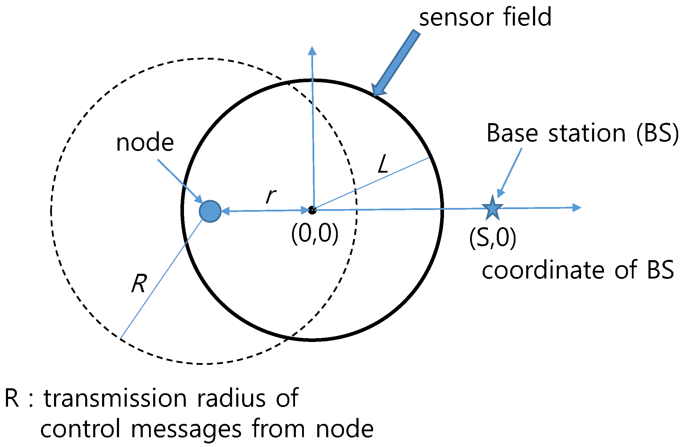
Consider the circular-shaped sensor field with radius of L (m) in Figure 1. The center of the sensor field is the origin (0, 0) of the coordinate system. Let S $(S\ge L)$ denote distance of BS from the center of the sensor field. The base station (BS) is considered to be at the border or outside of the sensor field at coordinate (S, 0). Within the sensor field, we have a node at r ($0<r<L$) (m) away from the origin (0, 0). Each node has transmission radius R ($L<R<2L$) for control messages including ADV, Join-REQ, and TDMA messages.

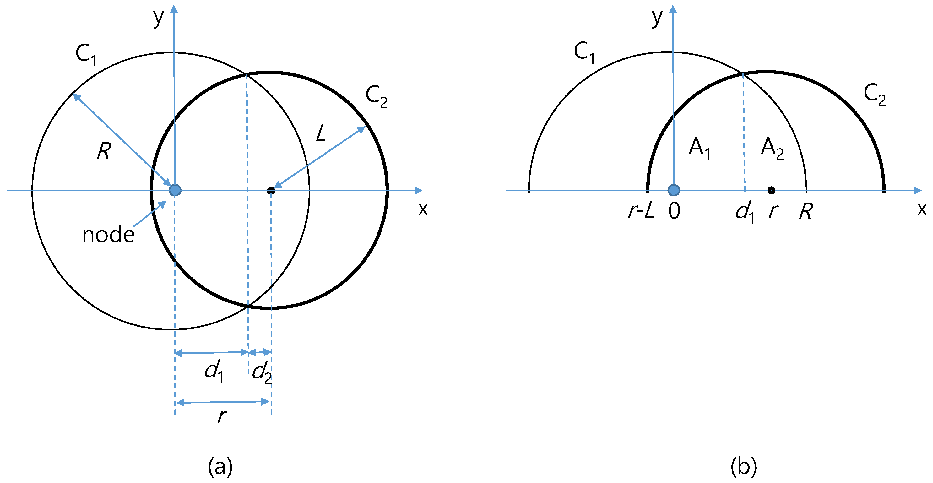
Consider a node marked at r ($0<r<L$) (m) away from the origin in Figure 1. Using a dashed circle, we show the transmission radius R (m) of control messages for the marked node. Inside of the sensor field, the area covered by the transmission range of the marked node is called effective area of the marked node. In the case of $0<r<R-L$, the marked node is close to the center of the sensor field. In this case, the transmission range depicted by the dashed circle includes the entire sensor field as in Figure 2a; and the effective area of the marked node is exactly the same as the entire sensor field. However, in the case of $R-L<r<L$, the sensor field is covered in part by the transmission range of the marked node as in Figure 2b, and the effective area of the node is the intersection of the two partially overlapping circles.

By assuming symmetrical propagation channel between any two nodes, a node can hear ADV messages from other nodes which only reside in its effective area. The effective area $A(r,R)$ of a node at r (m) $(0<r<L)$ away from the origin, with transmission range R, is calculated by (see Appendix A for its derivation)

$$A(r,R)=\left\{\begin{array}{cc}\pi L^2,& 0<r<R-L,\\ I(r,R),& R-L<r<L,\end{array}\right.$$

(4)

where

$$I(r,R)=R^2{cos}^{-1}\left(\frac{r^2+R^2-L^2}{2rR}\right)+L^2{cos}^{-1}\left(\frac{r^2+L^2-R^2}{2rL}\right)-\frac{1}{2}\sqrt{4r^2{L}^2-{(r^2-R^2+L^2)}^2}$$

is the intersection area of the two partially overlapped circles. The expectation, $\overline{A}\left(R\right)$, of the effective area is given by (see Appendix B for its derivation)

$$\begin{array}{c}\overline{A}\left(R\right)=\frac{1}{\pi L^2}{\int }_0^{2\pi }{\int }_0^{L}A(r,R)r\mathrm{d}r\mathrm{d}\theta \hfill \\ =\pi {(R-L)}^2+\frac{2}{L^2}{\int }_{R-L}^{L}I(r,R)r\mathrm{d}r\hfill \\ =2R^2{cos}^{-1}\left(\frac{R}{2L}\right)+L^2{cos}^{-1}\left(1-\frac{R^2}{2L^2}\right)-\frac{(2L^{2}R+R^3)\sqrt{4L^2-R^2}}{4L^2}.\hfill \end{array}$$

(5)

It is noted that Equation (5) is calculated by taking into account both the total inclusion and partial overlap cases to obtain the expectation of transmission range of an arbitrary node.

Given k and R, we consider the probability that a node hears ADV messages from n CHs as the probability that a node has n CHs in its effective area. We model this probability as the spatial Poisson process, which is a stationary two-dimensional Poisson point process successfully adopted in modeling wireless sensor networks [23,24,25]:

$$P_{k,R}^{\left(n\right)}=\frac{{\left\{\lambda \overline{A}\left(R\right)\right\}}^n}{n!}{\mathrm{e}}^{-\lambda \overline{A}\left(R\right)},$$

(6)

where the density, the number of sensor nodes per unit area,

$$\lambda =\frac{k}{\pi L^2}$$

is the average number of CHs within unit area. A node can join a cluster if it has heard from one of more CHs. Therefore, the probability that a node fails to join a cluster for the current round is given by the probability of hearing zero ADV message:

$$P_{k,R}^{\left(0\right)}={\mathrm{e}}^{-\frac{k}{\pi L^2}\overline{A}\left(R\right)}.$$

(7)

The length of ADV, Join-REQ, TDMA, and DATA messages are denoted by $l_A$, $l_J$, $l_T^{(k,R)}$, and $l_D$, respectively (in bits). Among them, lengths $l_A$, $l_J$, and $l_D$ are fixed. However, the length of a TDMA schedule message, $l_T^{(k,R)}$, depends on the number of member nodes in the current cluster, and the number of members, again, depends on $(k,R)$. The expected number of non-CH nodes which successfully join clusters is

$$(N-k)(1-P_{k,R}^{\left(0\right)}),$$

which, after dividing by k, gives the expected number of member nodes in a cluster. We have

$$l_T^{(k,R)}=\frac{16(N-k)(1-P_{k,R}^{\left(0\right)})}{k},$$

(8)

where 16 is assumed to be the number of bits to represent each node ID. In the following subsections, we analyze the overall amounts of energy that are expended by the nodes in a round as a function of k and R.

3.1. Energy Dissipation by Non-CH Nodes

In this subsection, we analyze the expected amount of energy consumed by non-CH nodes in a round. First, consider sending Join-REQ messages with transmission radius of R. Since we have $R>L$ and assume

$$L\gg \delta ,$$

the expectation of energy dissipation $E_{T-Join}$ by a non-CH node sending a Join-REQ message is given by

$$E_{T-Join}=(1-P_{k,R}^{\left(0\right)})l_J(E_e+{ϵ}_m{R}^4).$$

(9)

Modeling each of k clusters as a circle with the expectation of radius, $r_{CH}$, we calculate the area of each cluster as

$$\pi r_{CH}^2=\frac{\pi L^2}{k},$$

from which

$$r_{CH}=\frac{L}{\sqrt{k}}.$$

(10)

If we have $k<{(L/\delta )}^2$ then $r_{CH}>\delta$ and vice versa. Let $d_{CH}$ denote the distance from a member node to its CH. The expected amount of energy $E_{T-toCH}$ consumed by a member node while sending a DATA message to its CH is calculated by

$$E_{T-toCH}=(1-P_{k,R}^{\left(0\right)})l_D\left(E_e+{ϵ}_f\overline{d_{CH}^2}+{ϵ}_m\overline{d_{CH}^4}\right),$$

(11)

where, using Equation (10),

$$\begin{array}{c}\overline{d_{CH}^2}=\frac{2\pi }{\pi r_{CH}^2}{\int }_0^{\min (r_{CH},\delta )}{r}^3\mathrm{d}r\hfill \\ =\min \left(\frac{L^2}{2k},\frac{{\delta }^2}{2}\right),\hfill \end{array}$$

and

$$\begin{array}{c}\overline{d_{CH}^4}=\frac{2\pi }{\pi r_{CH}^2}{\int }_{\delta }^{\max (\delta ,r_{CH})}{r}^5\mathrm{d}r\hfill \\ =\max \left(\frac{L^6-k^3{\delta }^6}{3k^2{L}^2},0\right).\hfill \end{array}$$

We assume that the base station (BS) resides at coordinate $(S,0)$ where $S\ge L$. A non-CH node, failing to join a cluster, sends a DATA message to the BS directly, consuming the amount of energy $E_{T-toBS}$. Let $d_{BS}$ denote the distance from a node to the BS. With large fields, $E_{T-toBS}$ will be dominated by nodes with $d_{toBS}>\delta$, as follows.

$$\begin{array}{c}{E}_{T-toBS}=P_{k,R}^{\left(0\right)}{l}_D\left(E_e+{ϵ}_f\overline{d_{BS}^2}+{ϵ}_m\overline{d_{BS}^4}\right)\hfill \\ \simeq P_{k,R}^{\left(0\right)}{l}_D\left(E_e+{ϵ}_m\overline{d_{BS}^4}\right),\hfill \end{array}$$

(12)

where

$$\begin{array}{c}\overline{d_{BS}^4}=\frac{1}{\pi L^2}{\int }_{S-L}^{S+L}2x^5{cos}^{-1}\left(\frac{x^2+S^2-L^2}{2xS}\right)\mathrm{d}x\hfill \\ =S^4+2S^2{L}^2+\frac{L^4}{3},(S\ge L).\hfill \end{array}$$

(13)

The expectation of the number of CHs seen by a non-CH node is

$$\frac{k}{\pi L^2}\overline{A}\left(R\right).$$

The energy $E_{R-ADV}$ consumed by a non-CH node while receiving ADV messages is

$$E_{R-ADV}=\frac{k}{\pi L^2}\overline{A}\left(R\right)l_A{E}_e.$$

(14)

A non-CH node receives a TDMA scheduling message from its CH by expending energy $E_{R-TDMA}$:

$$E_{R-TDMA}=l_T^{(k,R)}{E}_e,$$

(15)

where $l_T^{(k,R)}$ is given in Equation (8).

Consequently, the expectation of total energy expended by all non-CH nodes in a round is given by

$$E_{non-CH}(k,R)=(N-k)\left(E_{T-Join}+E_{T-toCH}+E_{T-toBS}+E_{R-ADV}+E_{R-TDMA}\right).$$

(16)

3.2. Energy Dissipation by CH Nodes

We now analyze the expected amount of energy expended by CH nodes in a round. First, consider sending ADV and TDMA messages with transmission radius of R. Average amount of energy consumption by a CH node while transmitting ADV and TDMA messages are

$$E_{T-ADV}=l_A(E_e+{ϵ}_m{R}^4)$$

(17)

and

$$E_{T-TDMA}=l_T^{(k,R)}(E_e+{ϵ}_m{R}^4),$$

(18)

respectively.

The average number of member nodes of a CH is $(N-k)(1-P_{k,R}^{\left(0\right)})/k$. The expected data-aggregation energy by a CH node is

$$E_{Agg}=\left(1+\frac{(N-k)(1-P_{k,R}^{\left(0\right)})}{k}\right)l_D{E}_{DA}.$$

(19)

A CH node sends aggregated data to the BS by expending $E_{T-CHtoBS}$

$$E_{T-CHtoBS}=l_D\left(E_e+{ϵ}_m\overline{d_{BS}^4}\right),$$

(20)

where $\overline{d_{BS}^4}$ is calculated as in Equation (13).

In LEACH-based clustering protocol, a CH node receives other CHs’ ADV messages, although they are just dumped; we ignore the energy related to this step. A CH node will hear Join-REQ messages from all non-CH nodes in its control-message range, to check if they are destined for itself or not. Therefore, while a CH node receives Join-REQ messages, it consumes $E_{R-Join}$:

$$E_{R-Join}=l_J{E}_e(N-k)\frac{\overline{A}\left(R\right)}{\pi L^2}.$$

(21)

A CH requires energy $E_{R-DATA}$ during receiving DATA from its member nodes as follows:

$$E_{R-DATA}=\frac{(N-k)(1-P_{k,R}^{\left(0\right)})}{k}{l}_D{E}_e.$$

(22)

Consequently, the expectation of the total energy expended among all CH nodes in a round is given by

$$E_{CH}(k,R)=k\left(E_{T-ADV}+E_{T-TDMA}+E_{Agg}+E_{T-CHtoBS}+E_{R-Join}+E_{R-DATA}\right).$$

(23)

Finally, the expected amount of energy consumption in a round is

$$E(k,R)=E_{non-CH}(k,R)+E_{CH}(k,R).$$

(24)

4. Optimization of $(\mathit{k},\mathit{R})$

Our goal is to find the optimized $k_{opt}$ $(0<k_{opt}<N)$ and $R_{opt}$ $(L<R_{opt}<2L)$ to minimize $E(k,R)$ as in:

$$(k_{opt},R_{opt})=arg\underset{(k,R)}{min}E(k,R).$$

(25)

We note that $k_{opt}$ can be calculated as a real number, which can be readily applied to the LEACH algorithm by using rounding off form $[N/k]$ for the place of $N/k$ in the cluster-selection probability (Equation (3)).

Although $E(k,R)$ is high-order differentiable, getting gradients or Hessian matrix is expensive and complicated. Since $E(k,R)$ is observed to have convex-downward shape, as shown by the simulation presented below, we choose Nelder–Mead (N-M) Simplex algorithm [26,27], as a derivative-free optimization method. We suggest constructing the initial simplex as the following three vertices, ${\mathbf{v}}_1$, ${\mathbf{v}}_2$, and ${\mathbf{v}}_3$:

$$\begin{array}{c}{\mathbf{v}}_1=(k_1,R_1)=(5,\frac{3L}{2}),\hfill \\ {\mathbf{v}}_2=(k_2,R_2)=(5+{\Delta }_k,\frac{3L}{2}+{\Delta }_R),\hfill \\ {\mathbf{v}}_3=(k_3,R_3)=(5+{\Delta }_k,\frac{3L}{2}-{\Delta }_R),\hfill \end{array}$$

where ${\Delta }_k$ and ${\Delta }_R$ are 5% value of $k_1$ and $R_1$, respectively. In the first simplex ${\mathbf{v}}_1$, k is chosen to be 5 and R is taken as the mid-point of interval $[L,2L]$. Large-area sensor networks with large number of sensor nodes often show the optimum values of $k_{opt}$, which are greater than $k=5$ by conventional rule of thumb. Therefore, we suggest that both the second simplex ${\mathbf{v}}_2$ and the third, ${\mathbf{v}}_3$, have $k=5+{\Delta }_k$, instead of using conventional initialization with $k=5+{\Delta }_k$ for ${\mathbf{v}}_2$ and, $k=5-{\Delta }_k$ for ${\mathbf{v}}_3$.

The N-M optimization algorithm starts with the three vertices ${\mathbf{v}}_1$, ${\mathbf{v}}_2$, and ${\mathbf{v}}_3$. The function $E(k,R)$ takes on values $E\left({\mathbf{v}}_1\right)$, $E\left({\mathbf{v}}_2\right)$, and $E\left({\mathbf{v}}_3\right)$. The function values are to be compared to determine the best vertex, second best vertex, and the worst vertex. For N-M simplex transformations, we have used the standard values, 1, 1/2, 1, and 1/2 for the reflection, expansion, contraction, and shrink transformation, respectively. According to the N-M implementation in [27], we iteratively continue the ordering, centroid, and transformation steps of N-M algorithm with given termination tests to obtain the optimization value of ${\mathbf{v}}_{opt}=(k_{opt},R_{opt})$.

It is noted that the computational procedure for our proposed optimization described in this paper is not carried out by the sensor nodes, but is carried out at the base station (BS) and/or at the management center, which are assumed to have enough computational capabilities being supplied with sufficient power. The optimized parameters $(k_{opt},R_{opt})$ calculated at the management center can be implemented as a design parameter during the firmware installation for sensor nodes. The optimized parameters calculated at the BS can be broadcast to the sensor nodes deployed in the field through the wireless channel.

5. Performance Evaluation

In the performance evaluation, we used the lengths of messages as in the LEACH code [17]: $l_A=16$, $l_J=16$, and $l_D=8\times (500+25)$ (bits). We considered $N=100$ or $N=200$. We carried extensive simulations with large sizes of sensor fields, $L=\{200\mathrm{m},300\mathrm{m},400\mathrm{m}\}$, compared with the typical size of 100 m considered in most existing WSN routing protocols [3,18,19,20,21]. The unit of L and R is meters. We assumed $S=L$, i.e., the BS is on the boundary of the field.

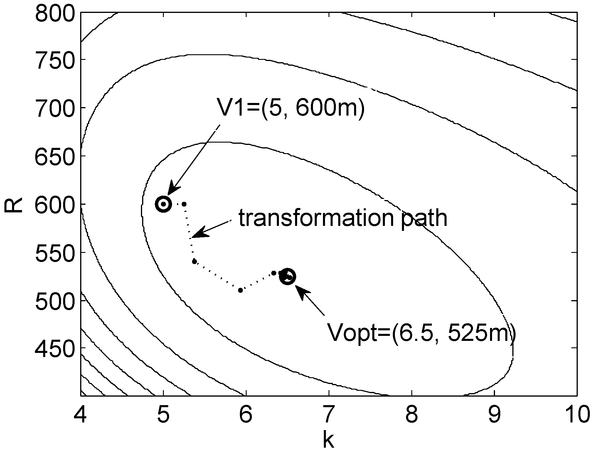
With our derived energy function $E(k,R)$, Nelder–Mead Simplex algorithm converged in an average of 50 iterations taking around 50 ms on a CPU running at 3.10 GHz. In Figure 3, we show a contour plot of $E(k,R)$ with $N=200$ and $L=400\mathrm{m}$. We also show the locations of initial simplex ${\mathbf{v}}_1=(5,600\mathrm{m})$ and the final optimized simplex ${\mathbf{v}}_{opt}=(6.5,525\mathrm{m})$ after 54 iterations. The marks connected with dotted lines between ${\mathbf{v}}_1$ and ${\mathbf{v}}_{opt}$ show the path of simplex transformations from the iterations of N-M optimization. A closer investigation on the convergence behavior of the N-M optimization process is shown in Appendix C. We observed that the iterations have 3 expansions, 9 reflections, 6 outside-contractions, and 36 inside-contractions out of a total of 54 transformations. Overall, 66% of transformations are inside-contractions, which means the energy function $E(r,R)$ has a very good shape for optimization.

We evaluated our proposed optimization by simulation with the LEACH code [17] from the originator, which runs on NS2 and has been verified in the literature, to obtain higher level of objectivity of our simulation results. For each scenario, we ran 100 simulations with different seed numbers to obtain narrow confidence intervals.

In

Table 2. Energy consumption per node in a round.

N	L	Energy Consumption (mJ)		Saving	$({\mathit{k}}_{\mathit{o}\mathit{p}\mathit{t}},{\mathit{R}}_{\mathit{o}\mathit{p}\mathit{t}})$
		Original LEACH [3]	LEACH w/Opt.
100	200 m	10.5	9.2	12.4%	(5.2, 286 m)
	300 m	31.9	24.1	24.5%	(5.2, 428 m)
	400 m	86.4	62.8	27.3%	(5.2, 571 m)
200	200 m	12.2	10.7	12.3%	(6.4, 263 m)
	300 m	31.2	20.3	34.9%	(6.5, 393 m)
	400 m	84.1	48.9	41.9%	(6.5, 525 m)

, we compare average energy consumption per node in a round with measure (mJ/node/round), between the original LEACH [3] and the LEACH with our optimization. Each value was obtained from several hundreds of rounds with all N nodes alive in the cluster-based routing algorithms. The larger are N and L, the higher is the percentage of energy savings. We also show the optimized parameters $(k_{opt},R_{opt})$ in the table as compared with the fixed values of $(k=5,R=2L)$ in the existing LEACH-based algorithms. It was observed that the optimum number k of clusters is dominated by N. On the other hand, R is mainly affected by the size, L, of sensor field.

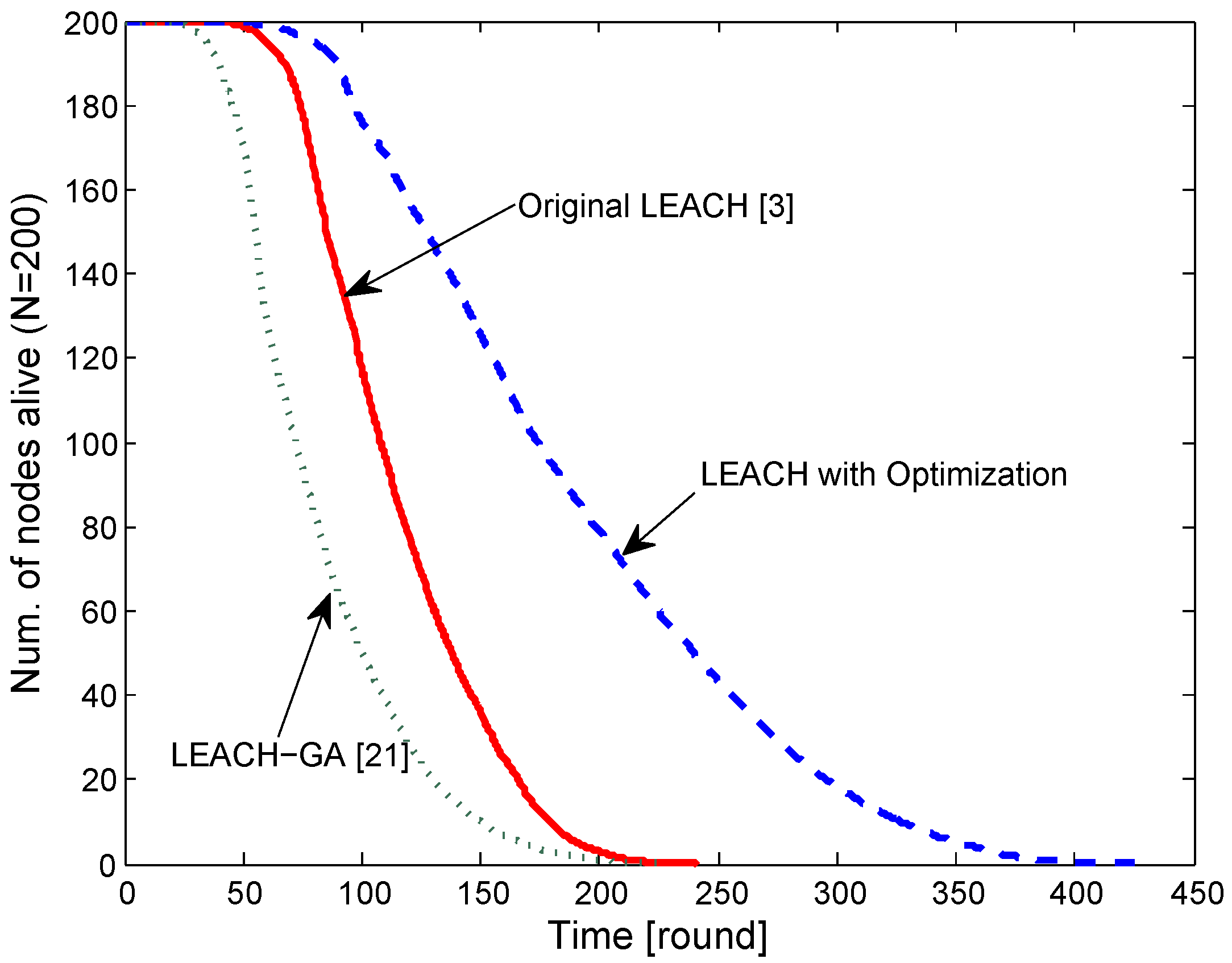
Figure 4 shows simulation results with $N=200$ and $L=400\mathrm{m}$. Every node had an initial energy of 10 (J). The original LEACH [3] takes $k=5$ by rule of thumb, and $R=2L=800\mathrm{m}$ to make sure that the entire sensor field is covered by any sensor node. In the figure, we show the number of nodes alive over simulation time in rounds. In the original LEACH [3], the average node lifespan is 110 rounds. Our proposed optimization, shown as “LEACH with Optimization”, takes $k_{opt}=6.5$ and $R_{opt}=525\mathrm{m}$ and outperforms the original, non-optimized LEACH [3] with an average node lifespan of 178 rounds, which is an increment of 62%. A genetic algorithm based optimization, LEACH-GA [21], does not take into account the energy dissipation for control messages, and yields an optimized value of $k=3.4$, which resulted in quick energy depletion in our simulation environment with large area sensor field.

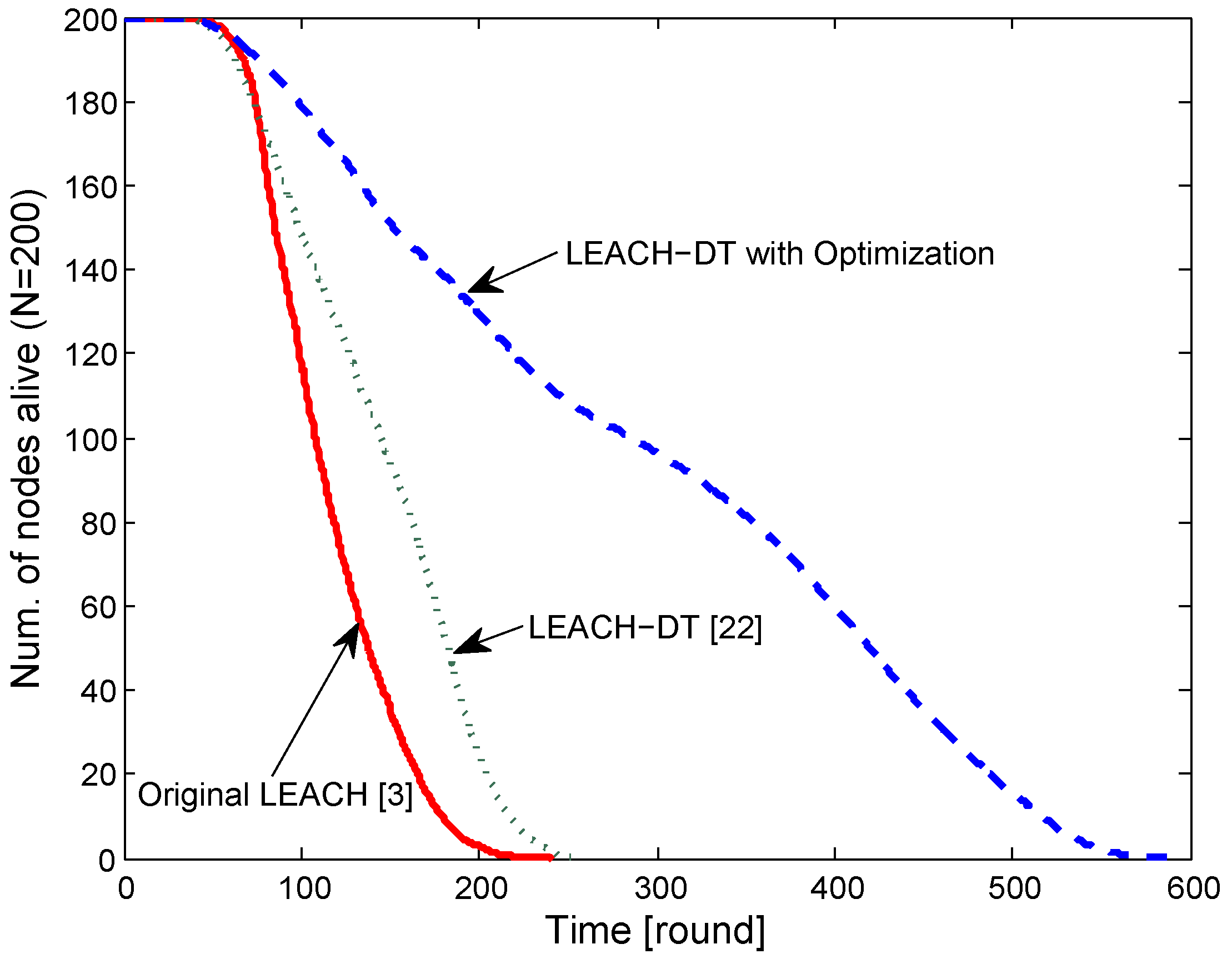
In Figure 5, we show how much our optimization improves another LEACH-based algorithm, LEACH-DT [22], which applies uneven probabilities to nodes in CH selection depending on the distance to the BS. LEACH-DT [22] uses the same parameters $k=5$ and $R=2L=800$ (m) as in the original LEACH. LEACH-DT itself outperforms the original LEACH, as shown in the figure. We could further improve LEACH-DT by running it with our optimized parameters $k_{opt}=6.5$ and $R_{opt}=525\mathrm{m}$, i.e., we used uneven CH-selection probabilities while keeping the average of 6.5 CHs in each round and setting the transmission radius for control messages to be 525 m. This improved LEACH-DT significantly, as shown in the curve “LEACH-DT with Optimization”.

In

Table 3. Time to percent-node-death.

Scheme		Time to %-Node-Death (Rounds)
		1%	10%	50%	90%
LEACH [3]	Non-opt.	54	74	108	166
	With opt.	68	97	174	296
LEACH-DT [22]	Non-opt.	47	73	146	205
	With opt.	51	98	286	488

, we compare performance in terms of time to percentage-node-death in rounds among the schemes compared in Figure 5. Our proposed optimization improved the network lifespan in terms of all criteria, 1–90%, in the table. We note that our optimization helps LEACH and LEACH-DT improve energy efficiency by increasing the lifespan dramatically with optimization. Consequently, our proposed optimization is expected to help existing cluster-based routing protocols to further improve in terms of network lifespan.

6. Conclusions

We have analyzed the expectation of energy dissipation in a round as a function of k and R to obtain joint optimization values of $(k_{opt},R_{opt})$. We have analyzed the amount of energy dissipation of CH nodes and non-CH nodes to derive the expectation of energy consumption in a round as a function of system design parameters $(k,R)$ with given network parameters including the number of sensor nodes N and the radius L of the sensor field. Our analyzed energy function is computationally tractable for derivative-free optimization algorithms, among which we adopt Nelder–Mead (N-M) simplex algorithm in our proposed scheme. The optimization procedure converges quickly enough for the BS or management center to run the optimization algorithm in real time. Our proposed method outperforms existing non-optimized LEACH-based schemes in terms of average node lifespan by saving the energy consumption by several tens of percent. Our optimization approach is expected to help existing cluster-based algorithms to further improve their energy efficiency.

References

1. Ghayvat, H.; Mukhopadhyay, S.; Gui, X.; Suryadevara, N. WSN- and IoT-based smart homes and their extension to smart buildings. Sensors 2015, 15, 10350–10379. [Google Scholar] [CrossRef] [PubMed]
2. Zhou, M.; Zhao, M.; Liu, A.; Ma, M.; Wang, T.; Huang, C. Fast and efficient data forwarding scheme for tracking mobile targets in sensor networks. Symmetry 2017, 9, 269. [Google Scholar] [CrossRef]
3. Heinzelman, W.B.; Chandrakasan, A.P.; Balakrishnan, H. An application-specific protocol architecture for wireless microsensor networks. IEEE Trans. Wirel. Commun. 2002, 1, 660–670. [Google Scholar] [CrossRef] [Green Version]
4. Essam, M.; Shaaban, E. Enhancing S-LEACH security for wireless sensor networks. Int. J. Appl. Comput. 2011, 4, 101–107. [Google Scholar]
5. Manzoor, B.; Javaid, N.; Rehman, O.; Akbar, M.; Nadeem, Q.; Iqbal, A.; Ishfaq, M. Q-LEACH: A new routing protocol for WSNs. Procedia Comput. Sci. 2013, 19, 926–931. [Google Scholar] [CrossRef]
6. Wang, A.; Yang, D.; Sun, D. A clustering algorithm based on energy information and cluster heads expectation for wireless sensor networks. Comput. Electr. Eng. 2012, 38, 662–671. [Google Scholar] [CrossRef]
7. Abdulsalam, H.M.; Ali, B.A. W-LEACH based dynamic adaptive data aggregation algorithm for wireless sensor networks. Int. J. Distrib. Sens. Netw. 2013, 9, 1–11. [Google Scholar] [CrossRef]
8. Sasikala, A.S.D.; Sangameswaran, N. Improving the energy efficiency of LEACH protocol using VCH in wireless sensor network. Int. J. Eng. Dev. Res. 2015, 3, 918–924. [Google Scholar]
9. Batra, P.K.; Kant, K. LEACH-MAC: A new cluster head selection algorithm for wireless sensor networks. Wirel. Netw. 2016, 22, 49–60. [Google Scholar] [CrossRef]
10. Liu, Y.; Xu, K.; Luo, Z.; Chen, L. A reliable clustering algorithm based on LEACH protocol in wireless mobile sensor networks. In Proceedings of the International Conference on Mechanical and Electrical Technology, Singapore, 10–12 September 2010; pp. 692–696. [Google Scholar]
11. Katiyar, V.; Chand, N.; Gautam, G.C.; Kumar, A. Improvement in LEACH protocol for large-scale wireless sensor networks. In Proceedings of the International Conference on Emerging Trends in Electrical and Computer Technology, Nagercoil, India, 23–24 March 2011; pp. 1070–1075. [Google Scholar]
12. Kim, D.S.; Cha, H.S.; Yoo, S. Improve far-zone LEACH protocol for energy conserving. In Proceedings of the International Conference on Wireless Communications, Networking and Mobile Computing, Shanghai, China, 21–23 September 2012; pp. 1–4. [Google Scholar]
13. Lee, J.Y.; Jung, K.D.; Moon, S.J.; Jeong, H.Y. Improvement on LEACH protocol of a wide-area wireless sensor network. Multimedia Tools Appl. 2017, 76, 19843–19860. [Google Scholar] [CrossRef]
14. Marappan, P.; Rodrigues, P. An energy efficient routing protocol for correlated data using CL-LEACH in WSN. Wirel. Netw. 2016, 22, 1415–1423. [Google Scholar] [CrossRef]
15. Cho, S.; Han, L.; Joo, B.; Han, S. P-LEACH: An efficient cluster-based technique to track mobile sinks in wireless sensor networks. Int. J. Distrib. Sens. Netw. 2014, 2014, 803656. [Google Scholar] [CrossRef]
16. Klaoudatou, E.; Konstantinou, E.; Kambourakis, G.; Gritzalis, S. A survey on cluster-based group key agreement protocols for WSNs. IEEE Commun. Surv. Tutor. 2011, 13, 429–442. [Google Scholar] [CrossRef]
17. MIT uAMPS LEACH ns Extentions. Available online: http://www2.ece.rochester.edu/projects/wcng/code.html (accessed on 1 December 2018).
18. Khediri, S.E.L.; Nasri, N.; Wei, A.; Kachouri, A. A new approach for clustering in wireless sensors networks based on LEACH. Procedia Comput. Sci. 2014, 32, 1180–1185. [Google Scholar] [CrossRef]
19. Devika, G.; Karegowda, A. A programatic study of LEACH and its decendant routing protocols in WSN. Int. J. Comput. Intell. Inform. 2015, 4, 300–307. [Google Scholar]
20. Singh, S.K.; Kumar, P.; Singh, J.P. A survey on successors of LEACH protocol. IEEE Access 2017, 5, 4298–4328. [Google Scholar] [CrossRef]
21. Liu, J.L.; Ravishankar, C.V. LEACH-GA: Genetic algorithm-based energy-efficient adaptive clustering protocol for wireless sensor networks. Int. J. Mach. Learn. Comput. 2011, 1, 79–85. [Google Scholar] [CrossRef]
22. Kang, S.H.; Nguyen, T. Distance based thresholds for cluster head selection in wireless sensor networks. IEEE Commun. Lett. 2012, 16, 1396–1399. [Google Scholar] [CrossRef]
23. Ram, S.S.; Manjunath, D.; Iyer, S.K.; Yogeshwaran, D. On the path coverage properties of random sensor networks. IEEE Trans. Mobile Comput. 2007, 6, 494–506. [Google Scholar] [CrossRef]
24. Liu, B.; Towsley, D. A study on the coverage of large-scale networks. In Proceedings of the IEEE International Conference on Mobile Ad-hoc and Sensor Systems, Fort Lauderdale, FL, USA, 25–27 October 2004; pp. 475–483. [Google Scholar]
25. Zhang, H.; Hou, J. On deriving the upper bound of α-lifetime for large sensor networks. In Proceedings of the 5th ACM International Symposium on Mobile Ad-Doc Networking and Computing, Tokyo, Japan, 24–26 May 2004; pp. 121–132. [Google Scholar]
26. Lagarias, J.C.; Reeds, J.A.; Wright, M.H.; Wright, P.E. Convergence Properties of the Nelder–Mead Simplex Method in Low Dimensions. SIAM J. Optim. 1998, 9, 112–147. [Google Scholar] [CrossRef]
27. Gao, F.; Han, L. Implementing the Nelder–Mead simplex algorithm with adaptive parameters. Comput. Optim. Appl. 2012, 51, 259–277. [Google Scholar] [CrossRef]
Figure 1. Sensor field and control-message transmission range.
Symmetry 11 00037 g001
Figure 2. Effective area of control-message.
Symmetry 11 00037 g002
Figure 3. Contour of energy function E ( k , R ) ( N = 200 , L = 400 m ) and N-M transformation path from initial simples v 1 = ( 5 , 600 m ) to optimized simplex v o p t = ( 6.5 , 525 m ) .
Symmetry 11 00037 g003
Figure 4. Number of nodes alive ( N = 200 , L = 400 m).
Symmetry 11 00037 g004
Figure 5. Number of nodes alive ( N = 200 , L = 400 m).
Symmetry 11 00037 g005