A Complex Lie-Symmetry Approach to Calculate First Integrals and Their Numerical Preservation

Abstract

We calculated Noether-like operators and first integrals of a scalar second-order ordinary differential equation using the complex Lie-symmetry method. We numerically integrated the equations using a symplectic Runge–Kutta method. It was seen that these structure-preserving numerical methods provide qualitatively correct numerical results, and good preservation of first integrals is obtained.

1. Introduction

Marius Sophus Lie proposed a symmetry-based method for the analytical solution of differential equations using groups of continuous transformations known as Lie groups [1,2,3,4]. Amalie Emmy Noether later presented her remarkable theorem that relates variational symmetries with conservation laws or first integrals in Reference [5]. In the literature, different methods are available to calculate first integrals of ordinary differential equations (ODEs), including the direct method, the characteristic or multiplier method, the Noether approach, and the partial Noether approach [6,7,8,9]. In this paper, we used the classical Noether approach to calculate the first integrals of a harmonic oscillator. We then applied the complex symmetry method in the restricted domain to find the first integrals of a system of harmonic oscillators by considering the Lagrangian in the complex variable domain [10,11,12].

Concerning the numerical solutions of ODEs with quadratic first integrals, it is well known that symplectic numerical methods are a suitable candidate [13]. These methods are a subclass of geometric integrators that preserve the geometric properties of the exact flow of ODEs. One class of symplectic methods with optimal order are the Gauss–Legendre Runge–Kutta methods. They are one-step numerical methods for ODEs and preserve all linear and quadratic first integrals of a dynamic system [14]. If we intend to preserve cubic or higher-order first integrals, we do not have a general numerical scheme for such a purpose, but we can design a numerical method that has this as its specific goal, for example, with the splitting and discrete-gradient methods [14]. In this paper, we present a way of constructing symplectic Runge–Kutta methods. We then take fourth-order Gauss–Legendre Runge–Kutta methods for the numerical integration of ODEs and report good preservation of first integrals by the numerical solution.

2. Symmetries and First Integrals

Consider a second-order ordinary differential equation,

$$\frac{d^{2}y}{dt}=f(t,y^{\prime },y),$$

(1)

which admits a Lagrangian L satisfying the Euler–Lagrange equation,

$$\frac{d}{dt}(\frac{\partial L}{\partial y^{\prime }})-\frac{\partial L}{\partial y}=0.$$

(2)

To explain the invariance criteria for variational problems under a group of transformation, we consider the operator

$$X=\xi (t,y)\frac{\partial }{\partial t}+\eta (t,y)\frac{\partial }{\partial y},$$

(3)

where X is the Noether symmetry generator for the Lagrangian L with gauge function $B(t,y)$, provided the following condition holds,

$$X^{(1)}(L)+D_t(\xi )L-D_t(B)=0,$$

(4)

where $X^{(1)}$ is a first-order prolongation of X and D represents total derivative,

$$D_t=\frac{\partial }{\partial t}+y^{\prime }\frac{\partial }{\partial y}.$$

(5)

According to the Noether theorem, for each Noether symmetry of a Euler–Lagrange equation, there corresponds a function I

$$I=\xi L+(\eta -\xi y^{\prime })\frac{\partial L}{\partial y^{\prime }}-B(t,y),$$

(6)

called the first integral or conserved quantity of Equation (1) with respect to symmetry generator X.

Complex Symmetry Analysis

We first discuss some important results related to complex Noether symmetries, complex Lagrangian, and the Noether theorem in the restricted complex domain. We use them to determine first integrals of second-order restricted complex ODEs [15]. We then present expressions for Euler–Lagrange-like equations, conditions for Noether-like operators, and expressions for first integrals corresponding to these operators. For more details, see Reference [10] and references therein.

Consider a system of two second-order ordinary differential equations of the form

$$\begin{array}{c}\hfill \begin{array}{cc}\hfill \frac{d^{2}f}{dt}& =w_1(t,g,f,g^{\prime },f^{\prime }),\hfill \\ \hfill \frac{d^{2}g}{dt}& =w_2(t,g,f,g^{\prime },f^{\prime }).\hfill \end{array}\end{array}$$

(7)

Suppose we have a transformation $y(t)=f+ig$ and $w=w_1+i{w}_2$, which converts System (7) to a second-order restricted complex ODE,

$$y^{″}=w(t,y,y^{\prime }).$$

(8)

Assume that Equation (8) admits a complex Lagrangian $L(t,f,g,f^{\prime },g^{\prime })$, i.e., $L=L_1+i{L}_2$. Therefore, we have two Lagrangians, $L_1$ and $L_2$, for System (7) that satisfy Euler–Lagrange-like equations:

$$\begin{array}{c}\hfill \begin{array}{cc}\hfill \frac{\partial L_1}{\partial f}+\frac{\partial L_2}{\partial g}-\frac{d}{dt}(\frac{\partial L_1}{\partial f^{\prime }}+\frac{\partial L_1}{\partial g^{\prime }})& =0,\hfill \\ \hfill \frac{\partial L_2}{\partial f}-\frac{\partial L_1}{\partial g}-\frac{d}{dt}(\frac{\partial L_2}{\partial f^{\prime }}-\frac{\partial L_1}{\partial g^{\prime }})& =0.\hfill \end{array}\end{array}$$

(9)

The operators

$$\begin{array}{c}\hfill \begin{array}{cc}\hfill X_1& ={\varsigma }_1\frac{\partial }{\partial t}+{\chi }_1\frac{\partial }{\partial f}+{\chi }_2\frac{\partial }{\partial g},\hfill \\ \hfill X_2& ={\varsigma }_2\frac{\partial }{\partial t}+{\chi }_2\frac{\partial }{\partial f}-{\chi }_1\frac{\partial }{\partial g}.\hfill \end{array}\end{array}$$

(10)

are called Noether-like operators for Lagrangians $L_1$ and $L_2$ such that:

$$\begin{array}{cc}\hfill -X_2^{(1)}(L_2)+X_1^{(1)}(L_1)+(D_t{\varsigma }_1)L_1-(D_t{\varsigma }_2)L_2& =D_t{A}_1,\hfill \\ \hfill X_2^{(1)}(L_1)+X_1^{(1)}(L_2)+(D_t{\varsigma }_1)L_2+(D_t{\varsigma }_2)L_1& =D_t{A}_2,\hfill \end{array}$$

(11)

where $A_1$ and $A_2$ are suitable gauge functions. The two first integrals corresponding to Noether-like operators $X_1$ and $X_2$ can be found as:

$$\begin{array}{cc}\hfill I_1& =-A_1+{\varsigma }_1{L}_1+{\partial }_{f^{\prime }}{L}_1({\chi }_1-{\varsigma }_2{L}_2-{\varsigma }_1{f}^{\prime }-{\varsigma }_2{g}^{\prime })-{\partial }_{f^{\prime }}{L}_2({\chi }_2-{\varsigma }_2{f}^{\prime }-{\varsigma }_1{g}^{\prime }),\hfill \\ \hfill I_2& =-A_2+{\varsigma }_1{L}_2+{\partial }_{f^{\prime }}{L}_2({\chi }_1+{\varsigma }_2{L}_1-{\varsigma }_1{f}^{\prime }-{\varsigma }_2{g}^{\prime })+{\partial }_{f^{\prime }}{L}_1({\chi }_2-{\varsigma }_2{f}^{\prime }-{\varsigma }_1{g}^{\prime }).\hfill \end{array}$$

(12)

3. Runge–Kutta Methods

Runge–Kutta methods [16] are one-step numerical methods for the approximate solution of IVPs:

$$y^{\prime }(t)=f(y(t)),y(t_0)=y_0,y(t)\in {\mathbb{R}}^n.$$

(13)

These methods provide approximation $y_n=y(t_n)$ of the exact solution $y(t)$ at time $t_n=nh$, where $n=0,1,\dots$ and h corresponds to the stepsize. The generalized form of an s-stage Runge–Kutta method is

$$\begin{array}{cc}\hfill Y_k& {\displaystyle =y_{n-1}+\sum _{i=1}^s{a}_{ki}hf(Y_i),k=1,\dots ,s,}\hfill \\ \hfill y_n& {\displaystyle =y_{n-1}+\sum _{l=1}^s{b}_{l}hf(Y_l),}\hfill \end{array}$$

(14)

with $b_i$ representing the weights and $c_i$, the nodes at which stages $Y_k$ are evaluated. A Runge–Kutta method can be represented by a Butcher tableau:

$$\begin{array}{cccc}{c}_1& a_{11}& \cdots & a_{1n}\\ ⋮& ⋮& \ddots & ⋮\\ c_n& a_{n1}& \cdots & a_{nn}\\ & b_1& \cdots & b_n\end{array}.$$

For explicit Runge–Kutta methods, we have $a_{ki}=0$ for $k\le i,$; otherwise, they are implicit.

3.1. Symplectic Runge–Kutta Methods

If Equation (13) has a quadratic first integral

$$I(y)=\langle y,Sy\rangle =y^{T}Sy,$$

where S is a symmetric square matrix, then we have

$$\langle y,f(y)\rangle =y^{T}Sf(y)=0.$$

We want to determine numerical solutions $y_n$ such that first integral $I(y)$ is preserved numerically, i.e.,

$$\langle y_n,S{y}_n\rangle =\langle y_{n-1},S{y}_{n-1}\rangle n=0,1,\dots .$$

It has been shown in References [17,18,19] that only symplectic Runge–Kutta methods preserve quadratic first integrals while numerically integrating System (13). Moreover, in this paper we are only considering implicit Runge–Kutta methods to check the numerical preservation of first integrals because explicit methods cannot be symplectic [20]. A Runge–Kutta method is symplectic if its coefficients satisfy the following condition [18,19,21]:

$$b_i{a}_{ij}+b_j{a}_{ji}-b_i{b}_j=0\forall j,i=1,\dots ,s,$$

(15)

which can be derived as follows.

Firstly, apply the Runge–Kutta method (14) to solve the IVP (13). The stage values are

$${\displaystyle Y_i=y_{n-1}+\sum _{j}h{a}_{ij}f(Y_j).}$$

Since

$$\begin{array}{cc}& \langle Y_i,Sf(Y_i)\rangle =0,\hfill \\ \hfill \Rightarrow & {\displaystyle \langle y_{n-1},Sf(Y_i)\rangle +\sum _{j}h{a}_{ij}\langle f(Y_j),Sf(Y_i)\rangle =0.}\hfill \end{array}$$

(16)

Moreover, for the output values, we have

$${\displaystyle y_n=y_{n-1}+\sum _{i=1}^s{b}_{i}hf(Y_i).}$$

Thus,

$$\begin{array}{cc}\hfill \langle y_n,S{y}_n\rangle & {\displaystyle =\langle y_{n-1},S{y}_{n-1}\rangle +h\sum _i{b}_i\langle y_{n-1},Sf(Y_i)\rangle }\hfill \\ & {\displaystyle +h\sum _j{b}_j\langle f(Y_j),S{y}_{n-1}\rangle +h^2\sum _{i,j}{b}_j{b}_i\langle f(Y_i),Sf(Y_j)\rangle .}\hfill \end{array}$$

(17)

Evidently from Systems (16) and (17), we have

$$\langle y_n,S{y}_n\rangle =\langle y_{n-1},S{y}_{n-1}\rangle ,$$

provided that

$$b_j{a}_{ji}+b_i{a}_{ij}-b_i{b}_j=0.$$

(18)

3.2. Construction of Symplectic RK Methods

Although there exist several techniques to construct symplectic RK methods in the literature [14,22], here we constructed symplectic Runge–Kutta methods with the help of a Vandermonde transformation. This was first discussed in reference [23].

A Vandermonde matrix is given as

$$V=\left[\begin{array}{cccc}1& c_1& \cdots & c_1^{n-1}\\ ⋮& ⋮& \ddots & ⋮\\ 1& c_n& \cdots & c_n^{n-1}\end{array}\right]=c_i^{j-1}.$$

Pre- and postmultiply, Vandermonde matrix V with symplectic condition (15) as

$$c_i^{k-1}(b_j{a}_{ji}+b_i{a}_{ij}-b_j{b}_i)c_j^{l-1}=0,\forall l,k,j,i=1,2,\dots ,s.$$

(19)

To construct methods with two stages ($s=2$), we consider

For $l,k=1$,

$$\sum _{i,j}(b_j{a}_{ji}+b_i{a}_{ij}-b_j{b}_i)=0.$$

(20)

For $l=1$ and $k=2,$

$$\sum _{i,j}(b_j{c}_j{a}_{ji}+b_i{a}_{ij}{c}_j-b_j{c}_j{b}_i)=0.$$

(21)

For $l=2$ and $k=1,$

$$\sum _{i,j}(b_i{a}_{ij}{c}_j+b_j{c}_j{a}_{ji}-b_i{b}_j{c}_j)=0.$$

(22)

For $l,k=2$,

$$\sum _{i,j}(b_i{c}_i{a}_{ij}{c}_j+b_j{c}_j{a}_{ji}{c}_i-b_i{c}_i{b}_j{c}_j)=0.$$

(23)

The following order two conditions must be satisfied.

$$\sum _j{b}_j=1,\sum _j{b}_j{c}_j=\frac{1}{2}.$$

(24)

Using Equation (24) in Equations (20)–(23), we have

$$\begin{array}{cc}\hfill {\displaystyle \sum _i{b}_i{c}_i}& =\frac{1}{2},\hfill \\ \hfill {\displaystyle \sum _{i,j=1}^2(b_i{a}_{ij}{c}_j+b_j{c}_j{a}_{ji})}& =\frac{1}{2},\hfill \\ \hfill {\displaystyle \sum _{i,j=1}^2(b_i{c}_i{a}_{ij}+b_j{a}_{ji}{c}_i)}& =\frac{1}{2},\hfill \\ \hfill {\displaystyle \sum _{i,j=1}^2{b}_i{c}_i{a}_{ij}{c}_j}& =\frac{1}{8}.\hfill \end{array}$$

If we take $b_i(c_i-c_1)=b_i{c}_i-b_i{c}_1)$ and take summation of i from 1 to 2, we get

$$b_2{c}_2-b_2{c}_1=\frac{1}{2}-c_1,$$

$$b_2=\frac{c_1-\frac{1}{2}}{c_1-c_2}.$$

Similarly,

$$b_1=\frac{c_2-\frac{1}{2}}{c_2-c_1}.$$

If we take the relation

$$b_i(c_j-c_1)a_{ij}(c_i-c_1)=b_i{c}_i{a}_{ij}{c}_j-b_i{c}_i{a}_{ij}{c}_1-b_i{a}_{ij}{c}_j{c}_1+b_i{a}_{ij}{c}_1{c}_1.$$

Thus, we get

$$a_{22}=\frac{\frac{1}{8}-\frac{c_1}{6}-\frac{c_1}{3}+\frac{c_1{c}_1}{2}}{b_2{(c_2-c_1)}^2}.$$

Similarly, we get

$$a_{11}=\frac{\frac{1}{8}-\frac{c_2}{6}-\frac{c_2}{3}+\frac{c_2{c}_2}{2}}{b_1{(c_1-c_2)}^2},$$

$$a_{21}=\frac{\frac{1}{8}-\frac{c_2}{3}-\frac{c_1}{6}+\frac{c_1{c}_2}{2}}{b_2(c_2-c_1)(c_1-c_2)},$$

$$a_{12}=\frac{\frac{1}{8}-\frac{c_1}{3}-\frac{c_2}{6}+\frac{c_1{c}_2}{2}}{b_1(c_2-c_1)(c_1-c_2)}.$$

Let us consider the shifted Legendre polynomials $P_t^{*}$ on the interval $[0,1]$,

$${\displaystyle P_t^{*}(y)=\sum _{n=0}^t\frac{t!}{2t}\left(\begin{array}{c}t\\ n\end{array}\right)\left(\begin{array}{c}t+n\\ n\end{array}\right){(-1)}^{t-n}{y}^n.}$$

For Gauss methods, we choose abscissa $c_i$ as zeros of $P_t^{*}$ which have an order $2t$. For Radau methods, we choose either $c_1=0$ or $c_t=1$, or both of them and then take for Radau I methods, the abscissa as the zeros of the polynomial $P_{t-1}^{*}(y)+P_t^{*}(y)$ of order $2t-1$. Similarly, for Radau II methods, we take the abscissa as the zeros of the polynomial $P_t^{*}(y)-P_{t-1}^{*}(y)$ of order $2t-1$. Moreover, for Lobatto III methods, we take the abscissa as the zeros of the polynomial $P_t^{*}(y)-P_{t-2}^{*}(y)$ of order $2t-2$. Thus, we have the following symplectic methods:

Gauss, s = 2:

$$\begin{array}{ccc}\hfill \frac{1}{2}-\frac{\sqrt{3}}{6}& \frac{1}{4}& \hfill \frac{1}{4}-\frac{\sqrt{3}}{6}\hfill \\ \hfill \frac{1}{2}+\frac{\sqrt{3}}{6}\hfill & \frac{1}{4}+\frac{\sqrt{3}}{6}& \hfill \frac{1}{4}\hfill \\ & \frac{1}{2}& \hfill \frac{1}{2}\hfill \end{array}$$

Radau I, s = 2:

$$\begin{array}{ccc}\hfill 0\hfill & \frac{1}{8}& \hfill \frac{-1}{8}\hfill \\ \hfill \frac{2}{3}\hfill & \frac{7}{24}& \hfill \frac{3}{8}\hfill \\ & \frac{1}{4}& \hfill \frac{3}{4}\hfill \end{array}$$

Radau II, s = 2:

$$\begin{array}{ccc}\hfill \frac{1}{3}\hfill & \frac{3}{8}& \hfill \frac{-1}{24}\hfill \\ \hfill 1\hfill & \frac{7}{8}& \hfill \frac{1}{8}\hfill \\ & \frac{3}{4}& \hfill \frac{1}{4}\hfill \end{array}$$

Similarly, we can construct methods with more stages and a higher order.

4. Construction of First Integrals and Their Numerical Preservation

We construct the first integrals of a system of harmonic oscillators (both coupled and uncoupled) determined by the second-order ODE:

$$y^{″}=-k^{2}y.$$

(25)

We take different values of k and y, as follows:

Case I: (${\mathit{k}}^{\mathbf{2}}=\mathbf{1}$ and $\mathit{y}$ is real)

When $k^2=1$ and $y(t)$ is real-valued, (25) becomes a one-dimensional harmonic oscillator equation:

$$y^{″}=-y,$$

(26)

that possesses the standard Lagrangian

$$L=\frac{y^{\prime 2}}{2}-\frac{y^2}{2}.$$

(27)

Taking the Lagrangian and inserting it in System (4) yields the following determining system of equations:

$$\begin{array}{c}\hfill \begin{array}{c}\hfill -\eta y+{\eta }_t{y}^{\prime }+({\eta }_y-\frac{1}{2}{\xi }_t)y^{\prime 2}-\frac{1}{2}{\xi }_y{y}^{\prime 3}-\frac{1}{2}{\xi }_t{y}^2-\frac{1}{2}{\xi }_y{y}^2{y}^{\prime }-B_t-y^{\prime }{B}_y=0.\end{array}\end{array}$$

(28)

Comparing different powers of $y^{\prime }$, we have a system of four partial differential equations whose solution gives rise to:

$$\begin{array}{cc}\hfill \xi (t,y)& =c_1+c_{2}sin(2t)+c_{3}cos(2t),\hfill \\ \hfill \eta (t,y)& =sint{c}_4+(cos(2t)y{c}_2-sin(2t)y{c}_3)+cost{c}_5,\hfill \\ \hfill B(t,y)& =-(c_{2}sin(2t)+c_{3}cos(2t))y^2+(c_{4}cost-c_{5}sint)y.\hfill \end{array}$$

(29)

We thus obtain the following 5-Noether symmetry generators:

$$\begin{array}{c}\hfill \begin{array}{cc}\hfill X_1& =\frac{\partial }{\partial t},\hfill \\ \hfill X_2& =sin(2t)\frac{\partial }{\partial t}+ycos(2t)\frac{\partial }{\partial y},\hfill \\ \hfill X_3& =cos(2t)\frac{\partial }{\partial t}-ysin(2t)\frac{\partial }{\partial y},\hfill \\ \hfill X_4& =cos(t)\frac{\partial }{\partial y},\hfill \\ \hfill X_5& =sin(t)\frac{\partial }{\partial y}.\hfill \end{array}\end{array}$$

(30)

Using Symmetries (30) and Lagrangian (27) in Noether’s Theorem (6), we obtain the following first integrals:

$$\begin{array}{c}\hfill \begin{array}{cc}\hfill I_1& =\frac{y^{\prime 2}}{2}+\frac{y^2}{2},\hfill \\ \hfill I_2& =ysint+y^{\prime }cost,\hfill \\ \hfill I_3& =-ycost+y^{\prime }sint,\hfill \\ \hfill I_4& =-\frac{1}{2}{y}^{\prime 2}cos2t-y{y}^{\prime }sin2t+\frac{1}{2}{y}^{2}cos2t,\hfill \\ \hfill I_5& =-\frac{1}{2}{y}^{\prime 2}sin2t+y{y}^{\prime }cos2t+\frac{1}{2}{y}^{2}sin2t.\hfill \end{array}\end{array}$$

(31)

Among these five first integrals, only two are independent [8]. We numerically integrate system (26) using a fourth-order Gauss $s=2$ symplectic Runge–Kutta method that we refer to from now on as Gauss2. We compare the results of the Gauss2 method with the famous symplectic Euler method [14], given as:

$$\begin{array}{cc}\hfill U_{n+1}& =U_n+hf(V_n),\hfill \\ \hfill V_{n+1}& =V_n-hg(U_{n+1}),\hfill \end{array}$$

for numerically integrating $U^{\prime }=f(V)$ and $V^{\prime }=g(U)$. We take stepsize $h=0.01$, and n = 10,000 number of steps. By employing symplectic integrators, we expect the first integrals of the system to be preserved by the numerical schemes, and this is what we have achieved. We look at the deviation of numerically evaluated first integral $I(y_n)$ from the actual value of first integral $I(y_0)$. We calculate error by taking the difference of the first integral evaluated at initial value $I(y_0)$ with the value of the first integral evaluated at all subsequent numerically approximated values $I(y_n)$ given by the formula Error $=|I(y_n)-I(y_0)|$. 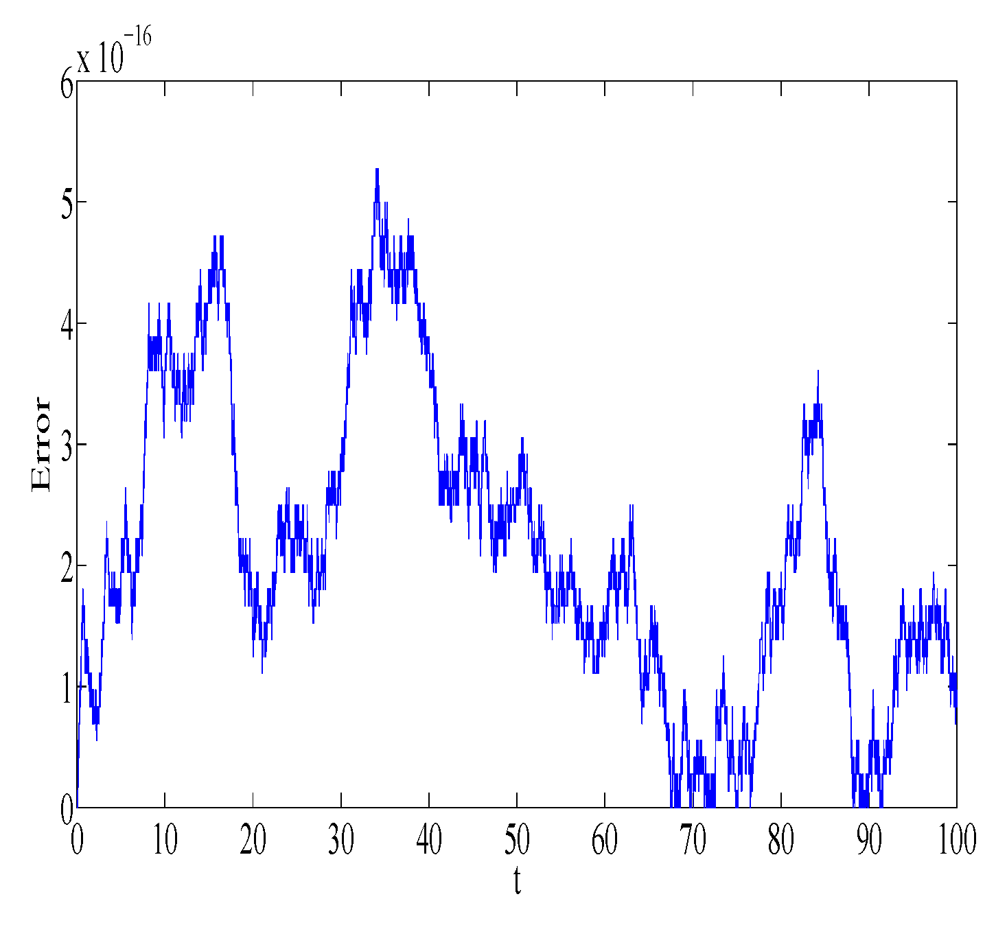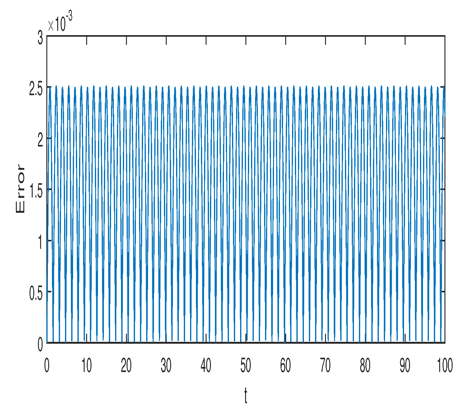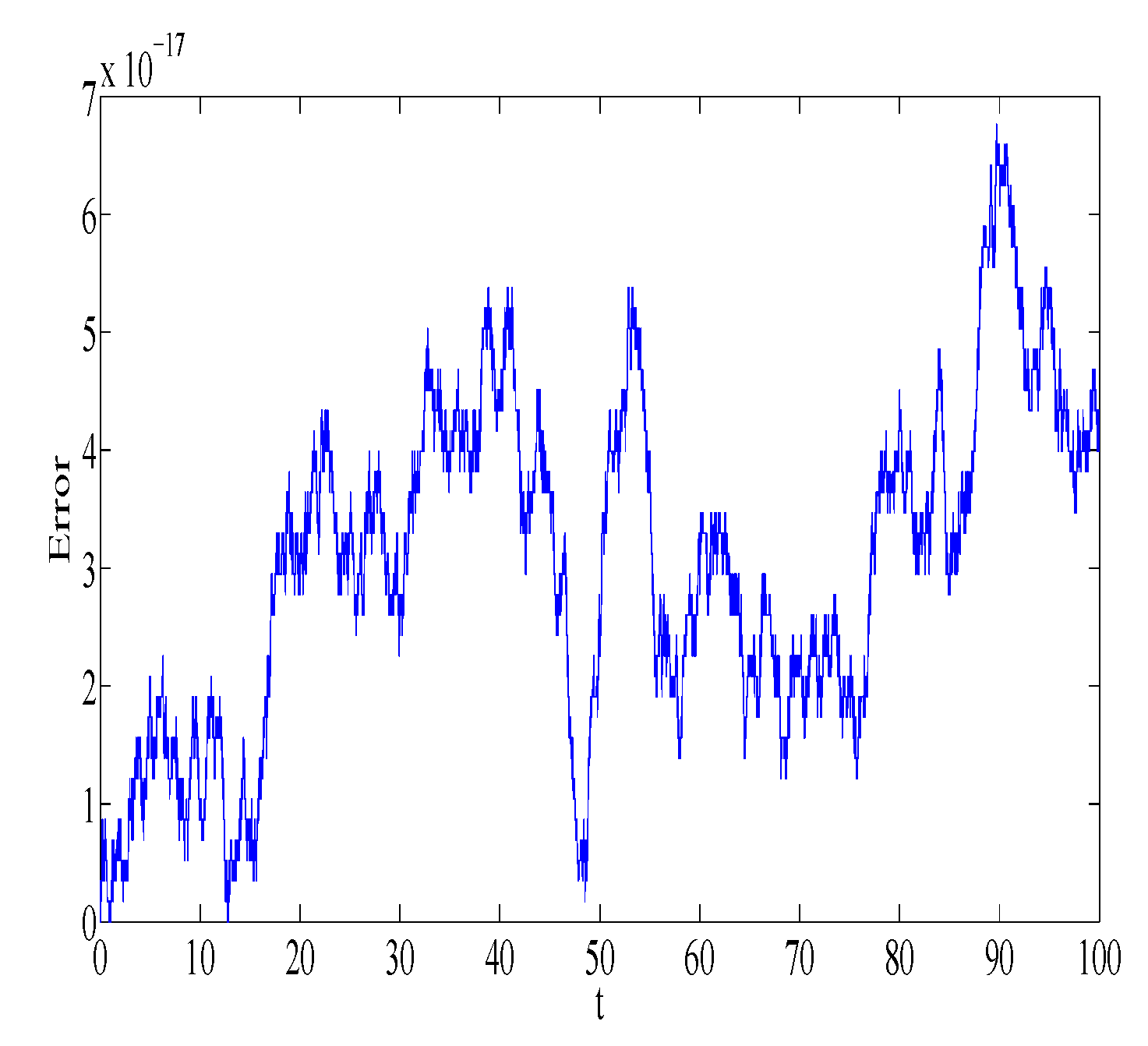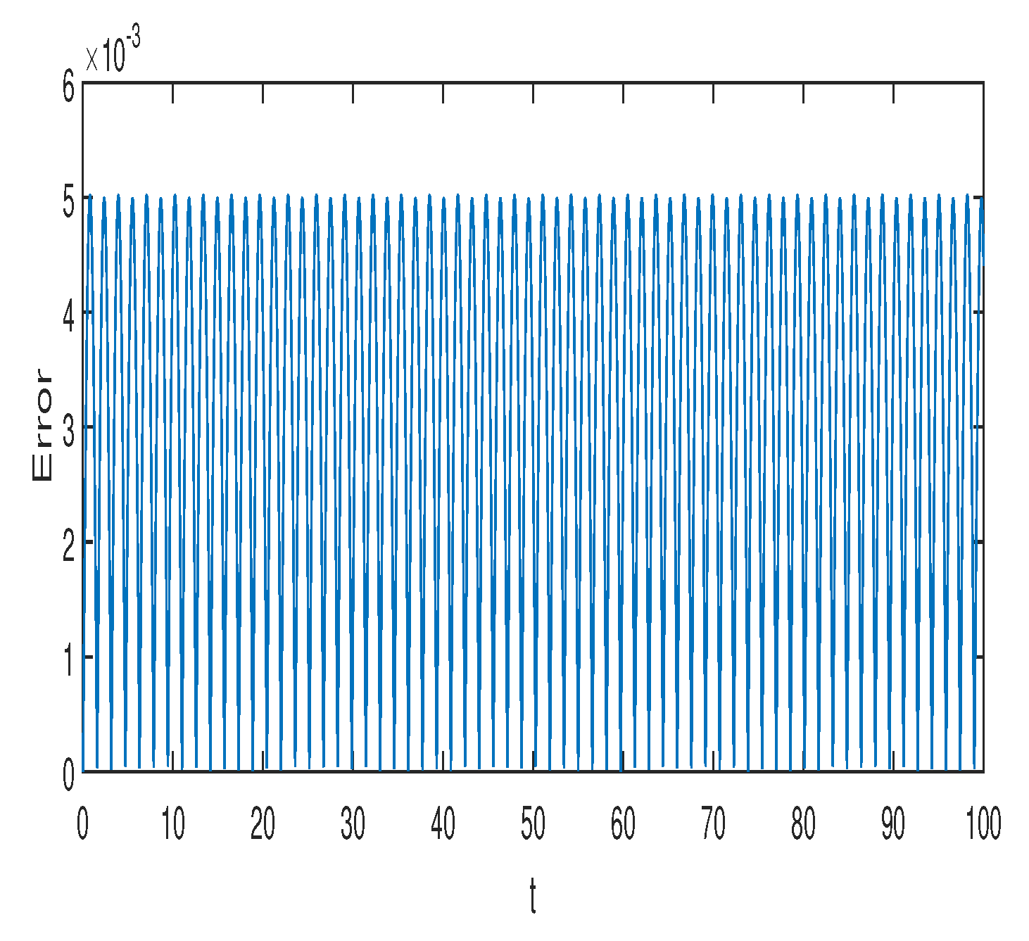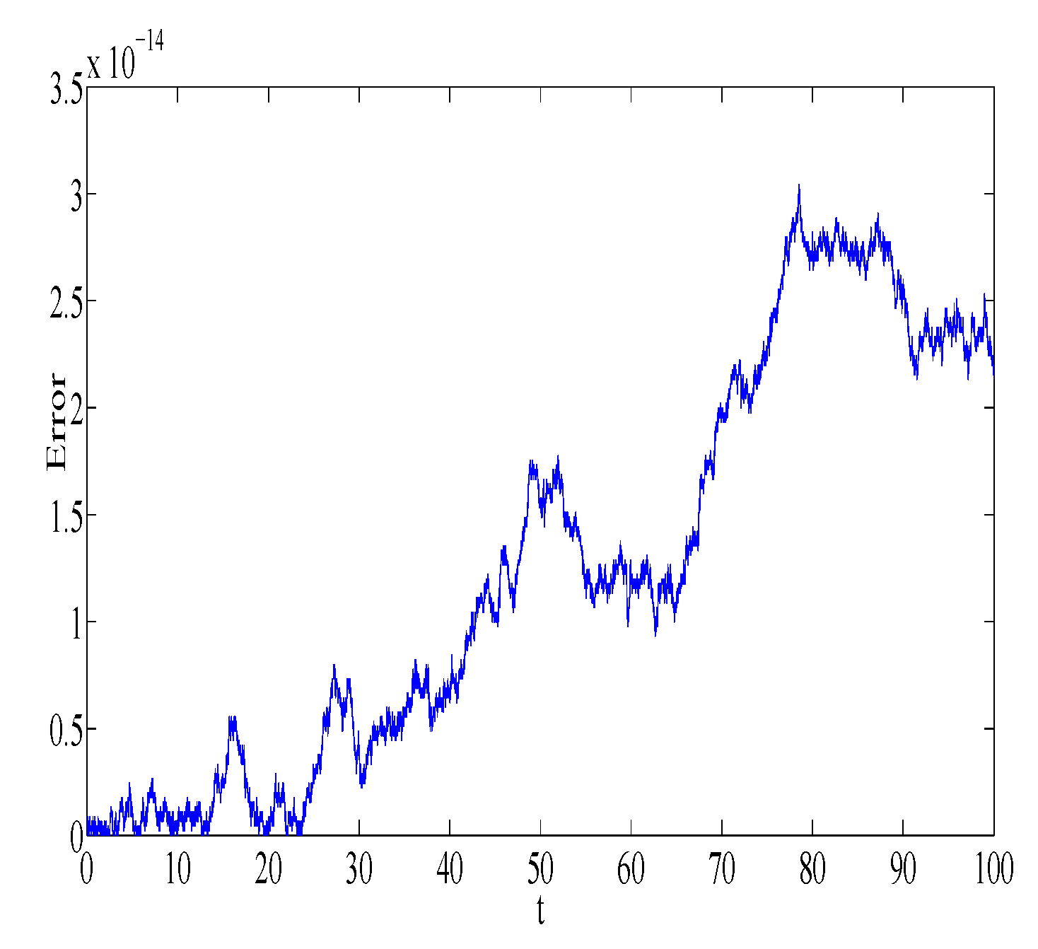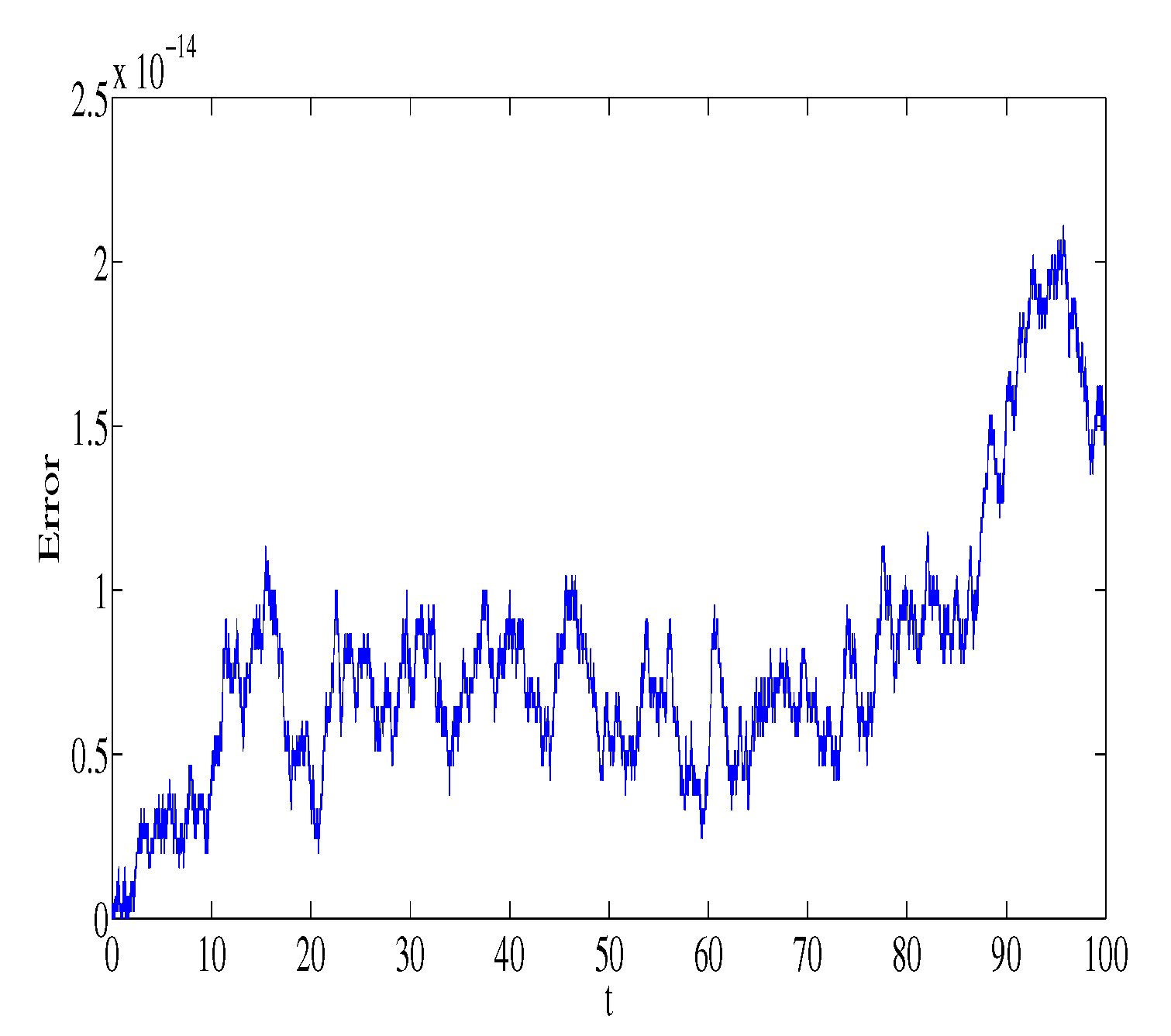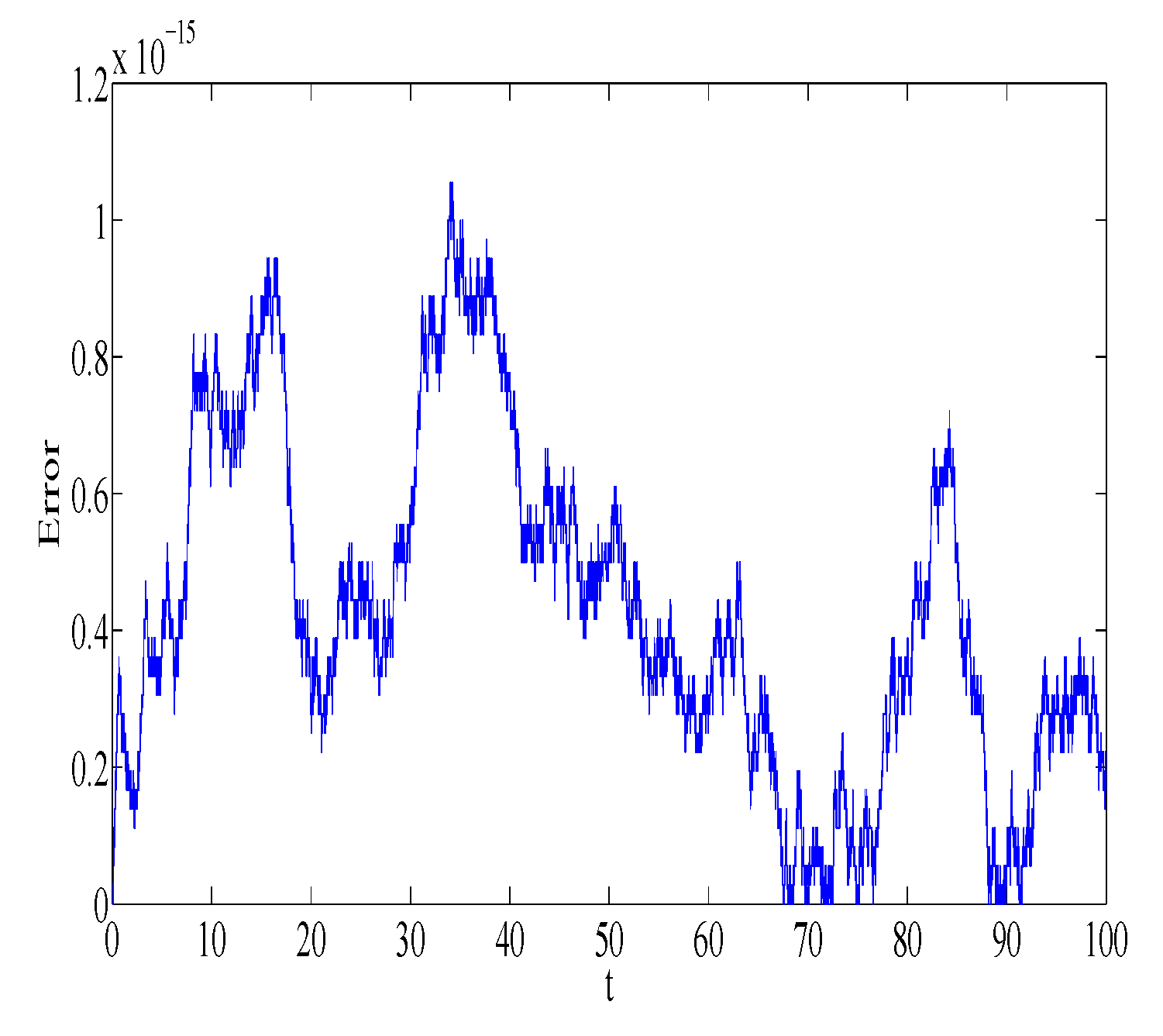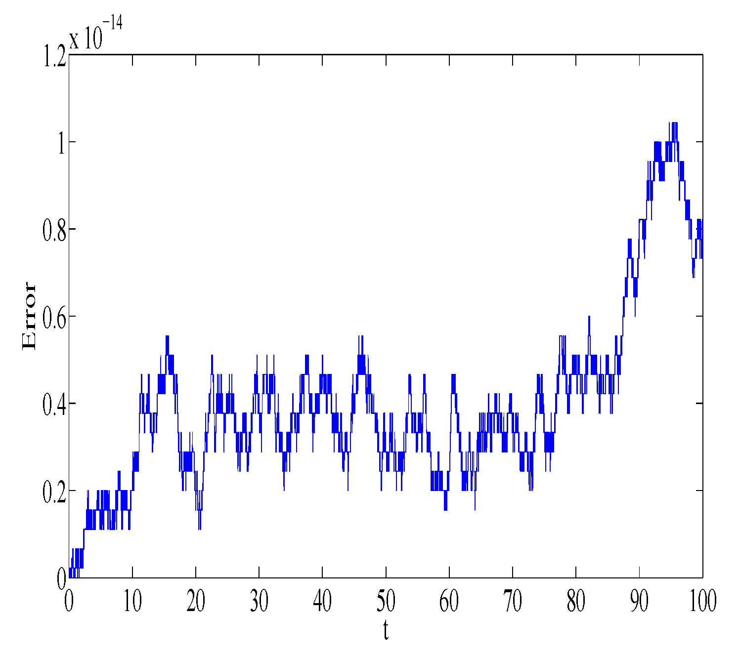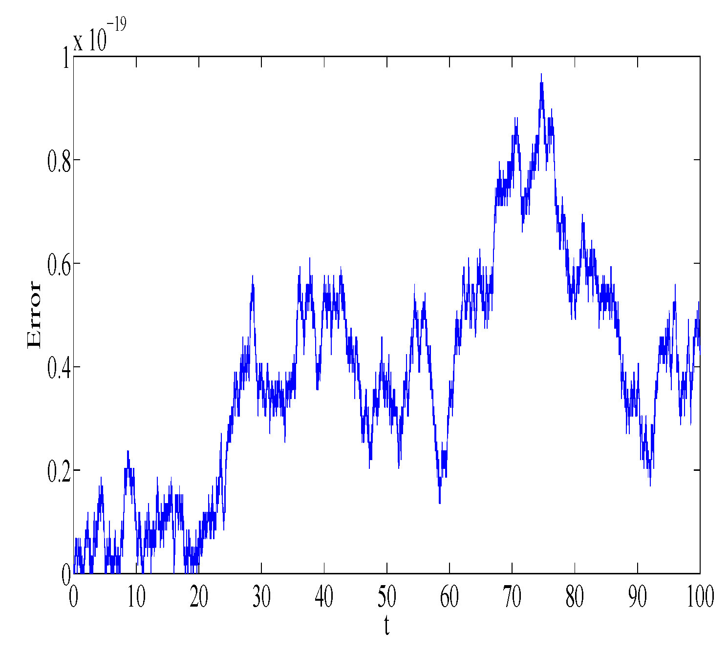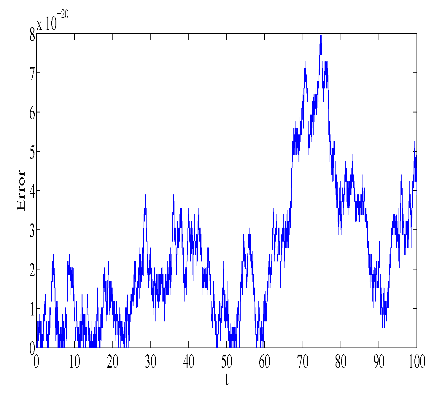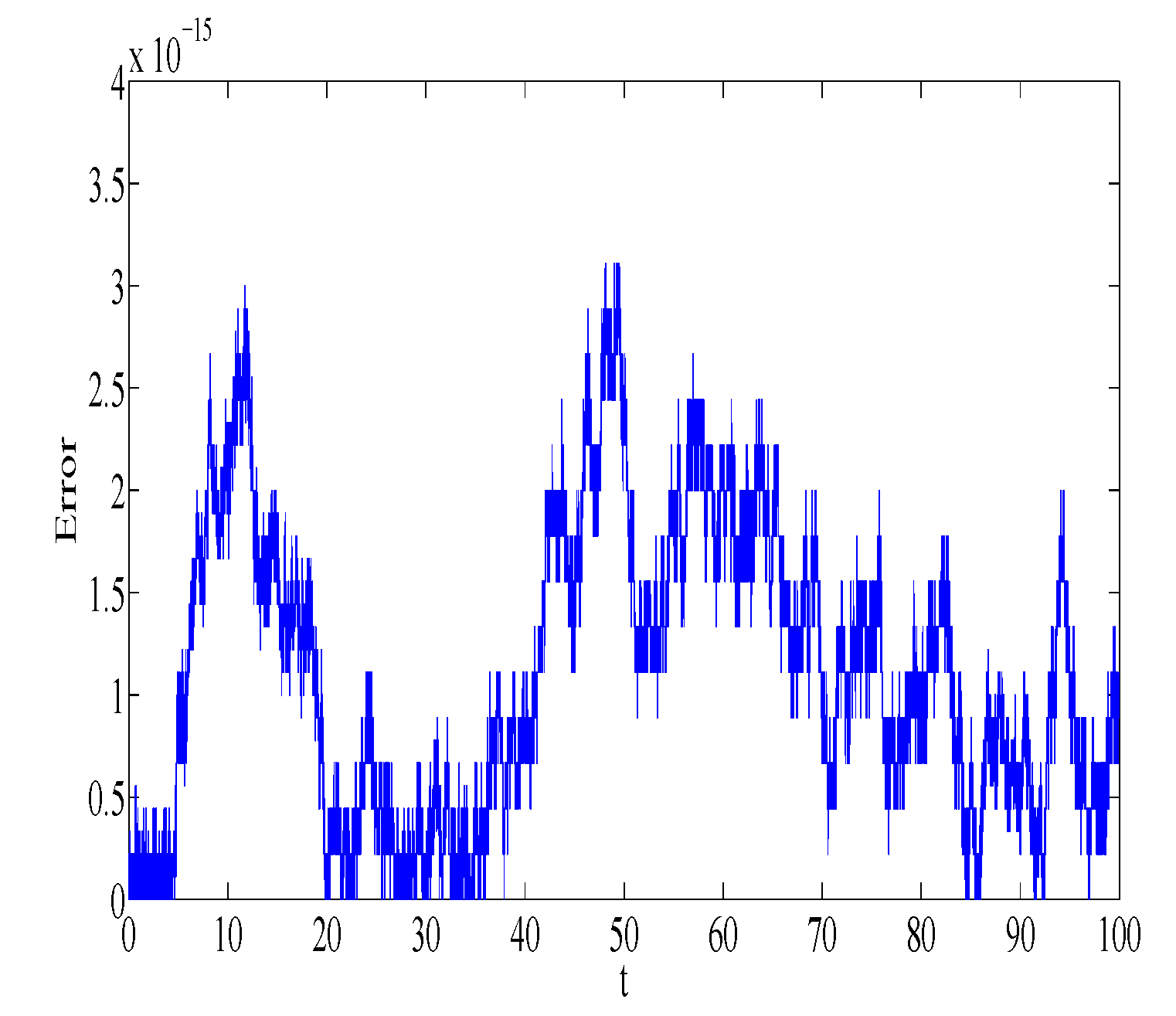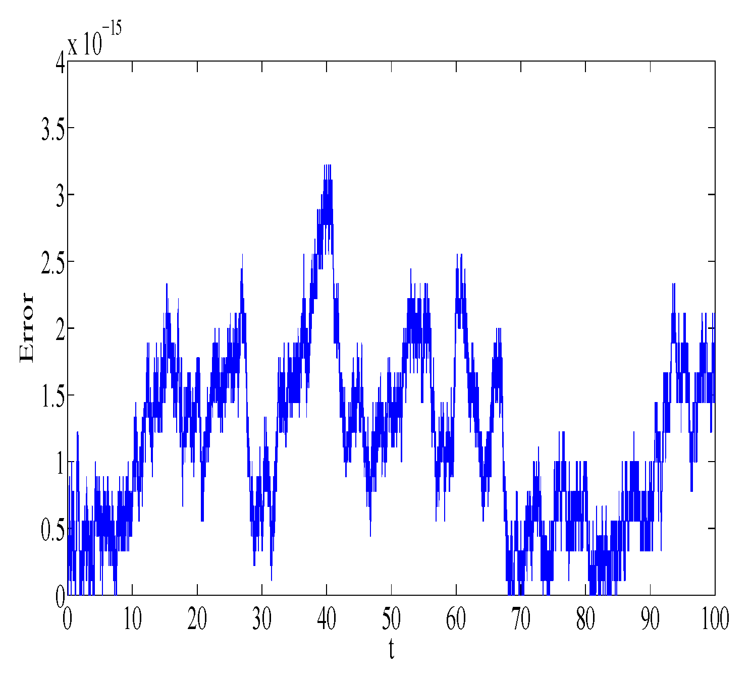Figure 1 and Figure 2 represent the absolute error in integral $I_2$ using the Gauss2 and symplectic Euler method, respectively. Similarly, Figure 3 and Figure 4 represent the absolute error in integral $I_3$ using the Gauss2 and symplectic Euler method, respectively. It is clear from the figures that the error is very small and bounded, depicting qualitatively correct numerical results. It is worth noting that the error of the Gauss2 method is much less compared to the error of the symplectic Euler method. The reason is that the Gauss2 method is fourth-order and more accurate compared to symplectic Euler method, which has order 1. Similar error behavior is obtained for other first integrals.

Case II: (${\mathit{k}}^{\mathbf{2}}=\mathbf{1}$ and $\mathit{y}$ is complex)

When $k^2=1$ and $y(t)$ is a complex function $y=f+ig$ for f and g being real functions of t, we get:

$$f^{″}=-f,g^{″}=-g,$$

(32)

which admits the following Lagrangians:

$$\begin{array}{cc}\hfill L_1& =\frac{1}{2}(-g^{\prime }{g}^{\prime }+f^{\prime }{f}^{\prime }-ff+gg),\hfill \\ \hfill L_2& =g^{\prime }{f}^{\prime }-fg.\hfill \end{array}$$

(33)

Using Lagrangians (33) in (11), we obtain 9-Noether-like operators

$$\begin{array}{cc}\hfill X_1& =\frac{\partial }{\partial t},X_2=sint\frac{\partial }{\partial f},X_3=sint\frac{\partial }{\partial g},X_4=cost\frac{\partial }{\partial f},X_5=cost\frac{\partial }{\partial g},\hfill \\ \hfill X_6& =sin2t\frac{\partial }{\partial t}+fcos2t\frac{\partial }{\partial f}+gcos2t\frac{\partial }{\partial g},\hfill \\ \hfill X_7& =gcos2t\frac{\partial }{\partial f}-fcos2t\frac{\partial }{\partial g},\hfill \\ \hfill X_8& =cos2t\frac{\partial }{\partial t}-fsin2t\frac{\partial }{\partial f}-gsin2t\frac{\partial }{\partial g},\hfill \\ \hfill X_9& =-gsin2t\frac{\partial }{\partial f}+fsin2t\frac{\partial }{\partial g}.\hfill \end{array}$$

(34)

Invoking Equation (12), we obtain the following invariants:

$$\begin{array}{cc}\hfill I_{1,1}& =(f^{\prime }{f}^{\prime }-g^{\prime }{g}^{\prime }-ff+gg)sin2t-2(f{f}^{\prime }-g{g}^{\prime })cos2t,\hfill \\ \hfill I_{1,2}& =2(f^{\prime }{g}^{\prime }-fg)sin2t-2(f{g}^{\prime }+f^{\prime }g)cos2t,\hfill \\ \hfill I_{2,1}& =(f^{\prime }{f}^{\prime }-g^{\prime }{g}^{\prime }-ff+gg)cos2t+2(f^{\prime }f-g^{\prime }g)sin2t,\hfill \\ \hfill I_{2,2}& =2(f^{\prime }{g}^{\prime }-fg)cos2t+2(f{g}^{\prime }+f^{\prime }g)sin2t,\hfill \\ \hfill I_{3,1}& =-2f^{\prime }cost-2fsint,\hfill \\ \hfill I_{3,2}& =-2g^{\prime }cost-2gsint,\hfill \\ \hfill I_{4,1}& =-2f^{\prime }sint+2fcost,\hfill \\ \hfill I_{4,2}& =-2g^{\prime }sint+2gcost,\hfill \\ \hfill I_{5,1}& =f^{\prime }{f}^{\prime }-g^{\prime }{g}^{\prime }-f^2+g^2,\hfill \\ \hfill I_{5,2}& =2g^{\prime }{f}^{\prime }+2gf.\hfill \end{array}$$

(35)

associated with Noether-like operators (34). System of Equation (32) is integrated using the Gauss2 method with stepsize $h=0.01$ and n = 10,000 number of steps. The absolute error in first integrals $I_{2,1}$, $I_{2,2}$, $I_{4,1}$, and $I_{4,2}$ is plotted in Figure 5, Figure 6, Figure 7 and Figure 8, respectively. Similar error behavior is obtained for $I_{1,1}$, $I_{1,2}$, $I_{3,1}$, $I_{3,2}$, $I_{5,1}$, and $I_{5,2}$. We observe that the error does not grow out of bounds, which shows that the numerical method can mimic the true qualitative feature of the dynamical system.

Case III: ($\mathit{k}$ and $\mathit{y}$ are complex)

When k and $y(t)$ are both complex, i.e., $k={\alpha }_1+i{\alpha }_2$ and $y=f+ig$ for f, g, ${\alpha }_1$, and ${\alpha }_2$ being real, the following coupled system of harmonic oscillators is obtained:

$$\begin{array}{cc}\hfill f^{″}& =-({\alpha }_1^2-{\alpha }_2^2)f+2{\alpha }_1{\alpha }_{2}g,\hfill \\ \hfill g^{″}& =-({\alpha }_1^2-{\alpha }_2^2)g-2{\alpha }_1{\alpha }_{2}f,\hfill \end{array}$$

(36)

which admits a pair of Lagrangians [11]:

$$\begin{array}{cc}\hfill L_1& =\frac{1}{2}{f}^{\prime 2}-\frac{1}{2}{g}^{\prime 2}-\frac{1}{2}({\alpha }_1^2-{\alpha }_2^2)(f^2-g^2)+2{\alpha }_1{\alpha }_{2}fg,\hfill \\ \hfill L_2& =f^{\prime }{g}^{\prime }-{\alpha }_1{\alpha }_2(f^2-g^2)-({\alpha }_1^2-{\alpha }_2^2)fg.\hfill \end{array}$$

(37)

System (36) admits the following 9 Noether-like operators and first integrals:

$$\begin{array}{cc}\hfill X_1& =\frac{\partial }{\partial t},\hfill \\ \hfill X_2& =sin({\alpha }_{1}t)cosh({\alpha }_{2}t)\frac{\partial }{\partial f}+cos({\alpha }_{1}t)sinh({\alpha }_{2}t)\frac{\partial }{\partial g},\hfill \\ \hfill X_3& =cos({\alpha }_{1}t)sinh({\alpha }_{2}t)\frac{\partial }{\partial f}-sin({\alpha }_{1}t)cosh({\alpha }_{2}t)\frac{\partial }{\partial g},\hfill \\ \hfill X_4& =cos({\alpha }_{1}t)cosh({\alpha }_{2}t)\frac{\partial }{\partial f}-sin({\alpha }_{1}t)sinh({\alpha }_{2}t)\frac{\partial }{\partial g},\hfill \\ \hfill X_5& =-sin({\alpha }_{1}t)sinh({\alpha }_{2}t)\frac{\partial }{\partial f}-cos({\alpha }_{1}t)cosh({\alpha }_{2}t)\frac{\partial }{\partial g},\hfill \\ \hfill X_6& =sin(2{\alpha }_{1}t)cosh(2{\alpha }_{2}t)\frac{\partial }{\partial t}+\{({\alpha }_{1}f-{\alpha }_{2}g)cos(2{\alpha }_{1}t)cosh(2{\alpha }_{2}t)\hfill \\ & +\{({\alpha }_{1}g+{\alpha }_{2}f)cos(2{\alpha }_{1}t)cosh(2{\alpha }_{2}t)-({\alpha }_{1}f-{\alpha }_{2}g)sin(2{\alpha }_{1}t)sinh(2{\alpha }_{2}t)\}\frac{\partial }{\partial g}\hfill \\ & +({\alpha }_{1}g+{\alpha }_{2}f)sin(2{\alpha }_{1}t)sinh(2{\alpha }_{2}t)\}\frac{\partial }{\partial f},\hfill \\ \hfill X_7& =cos(2{\alpha }_{1}t)sinh(2{\alpha }_{2}t)\frac{\partial }{\partial t}+\{({\alpha }_{1}g+{\alpha }_{2}f)cos(2{\alpha }_{1}t)cosh(2{\alpha }_{2}t)\hfill \\ & -\{({\alpha }_{1}f-{\alpha }_{2}g)cos(2{\alpha }_{1}t)cosh(2{\alpha }_{2}t)+({\alpha }_{1}g+{\alpha }_{2}f)sin(2{\alpha }_{1}t)sinh(2{\alpha }_{2}t)\}\frac{\partial }{\partial g}\hfill \\ & -({\alpha }_{1}f-{\alpha }_{2}g)sin(2{\alpha }_{1}t)sinh(2{\alpha }_{2}t)\}\frac{\partial }{\partial f},\hfill \\ \hfill X_8& =cos(2{\alpha }_{1}t)cosh(2{\alpha }_{2}t)\frac{\partial }{\partial t}+\{({\alpha }_{1}f-{\alpha }_{2}g)sin(2{\alpha }_{1}t)cosh(2{\alpha }_{2}t)\hfill \\ & +\{({\alpha }_{1}f-{\alpha }_{2}g)cos(2{\alpha }_{1}t)sinh(2{\alpha }_{2}t)+({\alpha }_{1}g+{\alpha }_{2}f)sin(2{\alpha }_{1}t)cosh(2{\alpha }_{2}t)\}\frac{\partial }{\partial g}\hfill \\ & -({\alpha }_{1}g+{\alpha }_{2}f)cos(2{\alpha }_{1}t)sinh(2{\alpha }_{2}t)\}\frac{\partial }{\partial f},\hfill \\ \hfill X_9& =-sin(2{\alpha }_{1}t)sinh(2{\alpha }_{2}t)\frac{\partial }{\partial t}+\{({\alpha }_{1}f-{\alpha }_{2}g)cos(2{\alpha }_{1}t)sinh(2{\alpha }_{2}t)\hfill \\ & -\{({\alpha }_{1}f-{\alpha }_{2}g)sin(2{\alpha }_{1}t)cosh(2{\alpha }_{2}t)-({\alpha }_{1}g+{\alpha }_{2}f)cos(2{\alpha }_{1}t)sinh(2{\alpha }_{2}t)\}\frac{\partial }{\partial g}\hfill \\ & +({\alpha }_{1}g+{\alpha }_{2}f)sin(2{\alpha }_{1}t)cosh(2{\alpha }_{2}t)\}\frac{\partial }{\partial f}.\hfill \end{array}$$

(38)

$$\begin{array}{cc}\hfill I_{1,1}& =({\alpha }_1^2-{\alpha }_2^2)(f^2-g^2)+f^{\prime 2}-4{\alpha }_1{\alpha }_{2}fg-g^{\prime 2},\hfill \\ \hfill I_{1,2}& =2({\alpha }_1^2-{\alpha }_2^2)fg+2{\alpha }_1{\alpha }_2(f^2-g^2)+2f^{\prime }{g}^{\prime },\hfill \\ \hfill I_{2,1}& =f^{\prime }sin({\alpha }_{1}t)cosh({\alpha }_{2}t)-g^{\prime }cos({\alpha }_{1}t)sinh({\alpha }_{2}t)-({\alpha }_{1}f-{\alpha }_{2}g)cos({\alpha }_{1}t)cosh({\alpha }_{2}t)\hfill \\ & -({\alpha }_{1}g+{\alpha }_{2}f)sin({\alpha }_{1}t)sinh({\alpha }_{2}t),\hfill \\ \hfill I_{2,2}& =g^{\prime }sin({\alpha }_{1}t)cosh({\alpha }_{2}t)+f^{\prime }cos({\alpha }_{1}t)sinh({\alpha }_{2}t)-({\alpha }_{1}g+{\alpha }_{2}f)cos({\alpha }_{1}t)cosh({\alpha }_{2}t)\hfill \\ & +({\alpha }_{1}f-{\alpha }_{2}g)sin({\alpha }_{1}t)sinh({\alpha }_{2}t),\hfill \\ \hfill I_{3,1}& =f^{\prime }cos({\alpha }_{1}t)cosh({\alpha }_{2}t)+g^{\prime }sin({\alpha }_{1}t)sinh({\alpha }_{2}t)+({\alpha }_{1}f-{\alpha }_{2}g)sin({\alpha }_{1}t)cosh({\alpha }_{2}t)\hfill \\ & -({\alpha }_{1}g+{\alpha }_{2}f)cos({\alpha }_{1}t)sinh({\alpha }_{2}t),\hfill \\ \hfill I_{3,2}& =g^{\prime }cos({\alpha }_{1}t)cosh({\alpha }_{2}t)-f^{\prime }sin({\alpha }_{1}t)sinh({\alpha }_{2}t)+({\alpha }_{1}g+{\alpha }_{2}f)sin({\alpha }_{1}t)cosh({\alpha }_{2}t)\hfill \\ & +({\alpha }_{1}f-{\alpha }_{2}g)cos({\alpha }_{1}t)sinh({\alpha }_{2}t),\hfill \\ \hfill I_{4,1}& =\frac{1}{2}[\{({\alpha }_1^2-{\alpha }_2^2)(-g^2+f^2)-4{\alpha }_1{\alpha }_{2}gf-(-g^{\prime 2}+f^{\prime 2})\}sin(2{\alpha }_{1}t)cosh(2{\alpha }_{2}t)\hfill \\ & -\{2{\alpha }_1{\alpha }_2{f}^2-2{\alpha }_1{\alpha }_2{g}^2+2({\alpha }_1^2-{\alpha }_2^2)gf-2g^{\prime }{f}^{\prime }\}cos(2{\alpha }_{1}t)sinh(2{\alpha }_{2}t)]\hfill \\ & +\{{\alpha }_1(f^{\prime }f-g^{\prime }g)-{\alpha }_2(g^{\prime }f+f^{\prime }g)\}cos(2{\alpha }_{1}t)cosh(2{\alpha }_{2}t)\hfill \\ & +\{{\alpha }_1{g}^{\prime }f+{\alpha }_1{f}^{\prime }g+{\alpha }_2{f}^{\prime }f-{\alpha }_2{g}^{\prime }g\}sin(2{\alpha }_{1}t)sinh(2{\alpha }_{2}t)\hfill \\ \hfill I_{4,2}& =\frac{1}{2}[\{({\alpha }_1^2-{\alpha }_2^2)(-g^2+f^2)-4{\alpha }_1{\alpha }_{2}gf+(g^{\prime 2}-f^{\prime 2})\}cos(2{\alpha }_{1}t)sinh(2{\alpha }_{2}t)\hfill \\ & +\{2{\alpha }_1{\alpha }_2(f^2-g^2)+2fg({\alpha }_1^2-{\alpha }_2^2)-2f^{\prime }{g}^{\prime }\}sin(2{\alpha }_{1}t)cosh(2{\alpha }_{2}t)]\hfill \\ & +[\{{\alpha }_1{f}^{\prime }g+{\alpha }_{1}f{g}^{\prime }+{\alpha }_2(f^{\prime }f-g{g}^{\prime })\}cos(2{\alpha }_{1}t)cosh(2{\alpha }_{2}t)]\hfill \\ & -[\{{\alpha }_{1}f{f}^{\prime }-{\alpha }_1{g}^{\prime }g)-{\alpha }_2{g}^{\prime }f-{\alpha }_2{f}^{\prime }g)\}sin(2{\alpha }_{1}t)sinh(2{\alpha }_{2}t)]\hfill \\ \hfill I_{5,1}& =\frac{1}{2}[\{({\alpha }_1^2-{\alpha }_2^2)(-g^2+f^2)-4{\alpha }_1{\alpha }_{2}fg-(-g^{\prime 2}+f^{\prime 2})\}cos(2{\alpha }_{1}t)cosh(2{\alpha }_{2}t)\hfill \\ & +\{2{\alpha }_1{\alpha }_2{f}^2-\{2{\alpha }_1{\alpha }_2{g}^2+2({\alpha }_1^2-{\alpha }_2^2)gf-2g^{\prime }{f}^{\prime }\}sin(2{\alpha }_{1}t)sinh(2{\alpha }_{2}t)]\hfill \\ & +\{{\alpha }_{1}f{g}^{\prime }+{\alpha }_{1}g{f}^{\prime }+{\alpha }_2(f{f}^{\prime }-g{g}^{\prime })\}cos(2{\alpha }_{1}t)sinh(2{\alpha }_{2}t)\hfill \\ & -\{-{\alpha }_1{g}^{\prime }g+{\alpha }_1{f}^{\prime }f-{\alpha }_{2}f{g}^{\prime }-{\alpha }_2{f}^{\prime }g\}sin(2{\alpha }_{1}t)cosh(2{\alpha }_{2}t)\hfill \end{array}$$

$$\begin{array}{cc}\hfill I_{5,2}& =\frac{1}{2}[\{-({\alpha }_1^2-{\alpha }_2^2)(-g^2+f^2)+4{\alpha }_1{\alpha }_{2}fg-g^{\prime 2}+f^{\prime 2}\}sin(2{\alpha }_{1}t)sinh(2{\alpha }_{2}t)\hfill \\ & +\{2{\alpha }_1{\alpha }_2(f^2-g^2)+2fg({\alpha }_1^2-{\alpha }_2^2)-2f^{\prime }{g}^{\prime }\}cos(2{\alpha }_{1}t)cosh(2{\alpha }_{2}t)]\hfill \\ & -[\{{\alpha }_1{f}^{\prime }g+{\alpha }_1{g}^{\prime }f-{\alpha }_2{f}^{\prime }f+{\alpha }_{2}g{g}^{\prime }\}sin(2{\alpha }_{1}t)cosh(2{\alpha }_{2}t)]\hfill \\ & -[\{{\alpha }_1{f}^{\prime }f-{\alpha }_1{g}^{\prime }g-{\alpha }_2{g}^{\prime }f-{\alpha }_2{f}^{\prime }g\}cos(2{\alpha }_{1}t)sinh(2{\alpha }_{2}t)]\hfill \end{array}$$

The Gauss2 method is again used to integrate Equation (36) with stepsize $h=0.01$ and n = 10,000 number of steps. The absolute error in the first integrals is calculated as before. The absolute error in integrals $I_{1,1}$, $I_{1,2}$, $I_{3,1}$ and $I_{3,2}$ is plotted in Figure 9, Figure 10, Figure 11 and Figure 12, respectively, which remains bounded for long time. Similar error behavior is obtained for $I_{2,1}$, $I_{2,2}$, $I_{4,1}$, $I_{4,2}$, $I_{5,1}$, and $I_{5,2}$. The symplectic Gauss2 method is able to preserve all first integrals obtained by performing complex symmetry analysis.

5. Conclusions

The first integrals of dynamical system $y^{″}=-k^{2}y$ were obtained via the classical Noether approach and the complex symmetry method. The later approach yields invariant energy as a particular example that is stored in both oscillators. Since these first integrals are quadratic in nature, the symplectic Runge–Kutta method, whose construction is also given in this paper, was successfully applied to the system, and numerical preservation of these first integrals was obtained. Interestingly, the numerical method presented in this paper could preserve the energy of the single oscillator as well as the energy stored in the pair of coupled oscillators that arise from the complex Noether approach. The error in the first integrals remained bounded for a long time, which would not have been possible if we have employed nonsymplectic integrators.