Article

Modeling and Control for a Multi-Rope Parallel Suspension Lifting System under Spatial Distributed Tensions and Multiple Constraints

1
School of Mechatronic Engineering, China University of Mining and Technology, Xuzhou 221116, China
2
Jiangsu Key Laboratory of Mine Mechanical and Electrical Equipment, China University of Mining and Technology, Xuzhou 221116, China
*
Author to whom correspondence should be addressed.
Symmetry 2018, 10(9), 412; https://doi.org/10.3390/sym10090412
Submission received: 21 August 2018 / Revised: 11 September 2018 / Accepted: 11 September 2018 / Published: 18 September 2018
(This article belongs to the Special Issue Symmetry and Engineering Design)

Abstract

:
The modeling and control of the multi-rope parallel suspension lifting system (MPSLS) are investigated in the presence of different and spatial distributed tensions; unknown boundary disturbances; and multiple constraints, including time varying geometric constraint, input saturation, and output constraint. To describe the system dynamics more accurately, the MPSLS is modelled by a set of partial differential equations and ordinary differential equations (PDEs-ODEs) with multiple constraints, which is a nonhomogeneous and coupled PDEs-ODEs, and makes its control more difficult. Adaptive boundary control is a recommended method for position regulation and vibration degradation of the MPSLS, where adaptation laws and a boundary disturbance observer are formulated to handle system uncertainties. The system stability is rigorously proved by using Lyapunov’s direct method, and the position and vibration eventually diminish to a bounded neighborhood of origin. The original PDEs-ODEs are solved by finite difference method, and the multiple constraints problem is processed simultaneously. Finally, the performance of the proposed control is demonstrated by both the results of ADAMS simulation and numerical calculation.

1. Introduction

The multi-rope parallel suspension lifting system (MPSLS) has many advantages over rigid robotic manipulators, such as lightweight characteristics, heavy payload capability, high transportability, and low energy consumption; which has gained much attention and has been addressed in numerous researches for decades [1,2]. The MPSLS consisting of a head sheave, a lifting rope with a lifting container attached at the bottom, two suspension ropes, and a sinking platform is illustrated in Figure 1. Such a multi-rope system has long flexible suspension ropes in parallel, moving towards deeper mine wells or ocean waters. Since the suspension rope of the multi-rope parallel suspension system is flexible, the transverse vibration of the flexible suspension rope induced by an unknown boundary disturbance, suggests that distributed and concentrated force is inevitable that limits the utility of the systems [3,4]. Transverse vibration of the system should be controlled and suppressed to avoid premature fatigue failure.
Given that the flexible suspension rope is a distributed parameter system, the model of the MPSLS derived from Hamilton’s principles is couple PDEs with infinite dimensions, which make it more difficult to control [5]. The general control methods, such as variable structure sliding-mode control [6], modal control [7], neural network control [8,9], etc. [10,11], can be used to suppress the vibration and improve the lifespan of the system, when the PDEs are discretized into ODEs by using Galerkin approximation method or finite element method [12]. There are still some shortcomings in these controls, such as modal spillover or restriction on a few critical modes [13]. In comparison, boundary control does not require distributed actuators and sensors, which is one of the most practical and efficient methods in extensive studies [14,15]. Active vibration control is introduced to achieve the vibration degradation [16], where both an unknown external disturbance and a spatiotemporally varying tension are considered. An Euler-Bernoulli beam system, together with the boundary feedback control, has been thoroughly studied by Guo [17], in which feedback states converge to any selected neighborhood of zero by both active disturbance rejection control and sliding mode control.
Nonlinear dynamics of hydraulic actuators and electric servomotors are generally subjected to a wide variety of constraints, including input saturation [18,19], dead zone [20], safety specification, and hysteresis [21,22], etc. Actual physical input saturation on hardware is typically denoted as a magnitude constraint on control input, such as the maximum thrust that a space thruster for a flexible aerial refueling hose can provide [23,24]. Based on the quaternion formulation of the dynamic equations, input saturation is recommended to reduce the actuation for unmanned aerial vehicles with a backstepping method [18]. A model reference adaptive control is investigated for a time-invariant system, where the plant is stable and of minimum phase with input saturation [19].
To avoid collisions between the sinking platform and other obstacles, the output constraint is considered in safety specifications of the MPSLS. In Reference [25], full-state feedback NN control combining with Barrier Lyapunov Function (BLF) is proposed for a serial mechanism with state constraints and no prior knowledge of the uncertainties. Adaptive fuzzy NN control is designed for a robot with unknown part, where a tan-type BLF is applied to ensure the boundedness of the output signal [26].
Although a great existing work for a single flexible distributed system, the research on multi-rope systems is limited at present [27,28]. In Reference [28], the modeling and control are investigated for a multi-rope system based on uniform tension string model and Lyapunov’s direct method [29], where the vessel position has been regulated by the proposed control. Then, on the base of that, the dynamics of the riser was taken into account in the top boundary control, where the undesirable vibration of the riser can be suppressed simultaneously [27]. The model of MPSLS is relatively complicated when the coupling among the sinking platform, the suspension rope, the lifting rope, and the lifting container are considered. In most of these works, boundary control laws are brought to merely achieve the purposes of vibration reduction for the multi-rope system, without non-uniform tension and multiple constraints. The main innovations are summarized as:
(1) Considering the couple relations of the suspension ropes with the lifting container and the sinking platform, a nonhomogeneous and coupled PDEs-ODEs model with different and spatial tensions is established to reflect the dynamic of the MPSLS.
(2) The model-based boundary control with input saturation and output constraint is proposed to reduce vibration for the MPSLS. An auxiliary function and an integral BLF are proposed to cope with the multiple constraints problem. Moreover, an adaptive observer is constructed to compensate for unknown boundary disturbance.
(3) A robust adaptive boundary control with two adaptive laws and a boundary disturbance observer is further redesigned to estimate correctly for unknown parameters of the system, and to compensate for an unknown boundary disturbance, respectively.
(4) The control performance achieved with the proposed control is verified by both the ADAMS simulation and numerical calculation in different cases. The parameter estimations quickly converge to actual values with the adaption laws.
The rest of the paper is organized as follows: A model is established to describe the MPSLS, in which both the couple relations of the suspension ropes with the lifting container and the sinking platform are considered explicitly in the geometric constraint in Section 2. Further, both two boundary control laws, including input saturation, output constraint, and boundary disturbance observer, are formulated in Section 3. The ADAMS simulation and numerical calculation are demonstrated to the efficiency and robustness of the control law in Section 4. Some conclusions are made in Section 5.

2. Modeling and Preliminaries

2.1. Modeling

The sinking platform is a secure essential equipment during vertical lift operations in deep mines or oceans, which is used to erect permanent supports and reinforcements and to secure the suspension cables of the lifting container. Main task of the container is lifting equipment or workers from the sinking platform or the sea bed. The suspension rope not only hangs on the sinking platform, but also acts as a guide role for the lifting container simultaneously. The top boundary of the suspension rope is connected to low speed winches for lifting the sinking platform to a new detective depth, as the working face advances.
External disturbances, including unknown time-varying boundary disturbance (such as, suspension equipment oscillating, uneven load distribution) and head sheave irregularities have been considered in the transverse vibration, which adds control difficulties for the MPSLS. The head sheave irregularities resulting from the inevitable error of manufacture and installation are a periodical excitation and a contributing factor, which results in vibration of the lifting rope. Control force is implemented at the bottom boundary of the sinking platform through actuators in transverse direction. Frame o x y z is the fixed inertia frame of the system.
Remark 1.
The transverse vibration of the distributed system depends on two independent variables: Spatial x and time t. y 0 ( x , t ) and y i ( x , t ) , i = 1 , 2 represent the transverse vibration of the lifting rope and the suspension rope, respectively, throughout this paper. For clarity, the notations are introduced as: ( · ) = ( x , t ) , ( · ) t = · / t , ( · ) x = · / x , ( · ) x t = 2 · / x t , ( · ) t t = 2 · / t 2 and ( · ) x x = 2 · / x 2 . The rest of the symbols are listed in the Nomenclature.
The kinetic energy of the MPSLS is given as
E k ( t ) = 1 2 ρ 1 0 l ( t ) ( y 0 , t + v y 0 , x ) 2 d x + i = 1 2 1 2 ρ 0 L y i , t 2 d x + 1 2 ( J θ ˙ 2 + m c ( y 0 , t + v y 0 , x ) 2 | x = l ( t ) + m y t 2 ( L , t ) )
The potential energy of the MPSLS is written as:
E p ( t ) = 1 2 0 l ( t ) T 0 ( x , t ) y 0 , x 2 d x + 1 2 i = 1 2 0 L T i ( x ) y i , x 2 d x
where T 0 ( x , t ) and T i ( x ) represent tension in the lifting and suspension rope, respectively, given by:
T 0 ( x , t ) = [ m c + ρ 1 ( l ( t ) x ) ] ( g a ) , 0 x l ( t )
T 1 ( x ) = ( D 2 D 1 + D 2 m + ρ ( L x ) ) g , T 2 ( x ) = ( D 1 D 1 + D 2 m + ρ ( L x ) ) g
The virtual work of the lifting container, the lifting rope, the suspension rope, and the sinking platform can be represented as:
δ W d ( t ) = c c ( y 0 , t ( x , t ) + v y 0 , x ( x , t ) ) | x = l c θ θ ˙ c y t ( L , t ) c 0 0 l ( t ) ( y 0 , t + v y 0 , x ) 2 d x i = 1 2 c i 0 L y i , t d x
The virtual work is given as:
δ W f ( t ) = i = 1 n 0 L f i ( t ) δ y i ( l , t ) δ ¯ ( x l ) d x + ( d ( t ) + u ( t ) ) δ y ( L , t ) + i = 1 n f i ( t ) δ y 0 ( l , t ) + 1 2 ( D 1 + D 2 ) · ( f 1 f 2 ) δ θ
Combining Equations (5) with (6), the total virtual work can be calculated by
δ W ( t ) = δ W f ( t ) + δ W d ( t )
Substituting Equations (1), (2) and (7) into the Hamilton’s principle, we have
t 1 t 2 ( δ E k ( t ) δ E p ( t ) + δ W ( t ) ) d t = t 1 t 2 ( i = 1 n 0 L A i δ y i ( x , t ) d x + 0 l ( t ) F δ y 0 ( x , t ) d x + H δ θ + S δ y 0 ( l , t ) + Q δ y ( L , t ) ) d t
where,
A i = ρ y i , t t + c i y i , t ( T i ( x ) y i x ) x + f i ( t ) δ ¯ ( x l ) F = ρ 1 ( y 0 , t t + 2 v y 0 , x t + v 2 y 0 , x x + a y 0 , x ) + c 0 ( y 0 , t + v y 0 , x ) ( T 0 ( x , t ) y 0 , x ) x H = J θ ¨ + c c θ ˙ ( D 1 + D 2 ) / 2 ( f 1 ( t ) f 2 ( t ) ) S = m ( y 0 , t t + 2 v y 0 , x t + v 2 y 0 , x x + a y 0 , x ) + c c ( y 0 , t + v y 0 , x ) + T 0 ( x , t ) y 0 , x i = 1 2 f i ( t ) Q = m y t t + c y t + i = 1 n T i ( x ) y i , x ( d ( t ) + u ( t ) )
Since δ [ · ] is an independent variation and must equal to zero during any time interval [ t 1 , t 2 ] , then A i = F = H = S = Q = 0 . The governing equations of the MPSLS are derived as follows:
ρ y i , t t + c i y i , t ( T i ( x ) y i x ) x + f i ( t ) δ ¯ ( x l ) = 0 , i = 1 , 2
ρ 1 ( y 0 , t t + 2 v y 0 , x t + v 2 y 0 , x x + a y 0 , x ) + c 0 ( y 0 , t + v y 0 , x ) ( T 0 ( x , t ) y 0 , x ) x = 0 ,
Boundary conditions of the lifting container and the sinking platform can be written as:
J θ ¨ + c θ θ ˙ = ( D 1 + D 2 ) ( f 1 ( t ) f 2 ( t ) ) / 2 ,
( m ( y 0 , t t + 2 v y 0 , x t + v 2 y 0 , x x + a y 0 , x ) + c c ( y 0 , t + v y 0 , x ) + T 0 ( x , t ) y 0 , x ) | x = l ( t ) = i = 1 2 f i ( t ) ,
( m y t t + c y t + i = 1 n T i ( x ) y i , x ) | x = L = d ( t ) + u ( t ) ,
y 1 ( 0 , t ) = y 2 ( 0 , t ) = 0 ,
y 0 ( l , t ) + r θ = y 1 ( l , t ) , y 0 ( l , t ) r θ = y 2 ( l , t )
y i ( L , t ) = y ( L , t ) , y i , t ( L , t ) = y t ( L , t ) ,
y 0 ( 0 , t ) = e ( t )
Equations (14)—(16) represent the boundary conditions of the suspension rope, the lifting container, the sinking platform, respectively. The top boundary disturbance of the lifting rope due to head sheave irregularities is denoted by e ( t ) as Equation (17).

2.2. Preliminaries

The following section provides some necessary assumptions and lemmas for stability analysis of the control design.
Remark 2.
The suspension rope tensions Equation (4) based on the geometric and mechanics relations between the suspension ropes and the sinking platform are non-uniform due to the spatial varying tensions. In addition, the lifting container with time-varying length restricted the displacement of two suspension ropes dynamically, and even severely impeded research on the problem of the multi-rope system. The MPSLS governed by Equations (9)–(17) is non-uniform, and the existing schemes for the uniform of PDEs cannot be applied directly.
Remark 3.
A nonhomogeneous and coupled PDEs-ODEs Equations (9)–(17) is used to describe the model of the MPSLS with time-varying geometric constraint and boundary disturbance, which is quite different from the model with a simple form [30]. Thus, another innovation of the paper is the consideration of the multiple constraints in the boundary control for the MPSLS.
Assumption 1.
The MPSLS suffers from the boundary disturbances. Assuming that the boundary disturbances and time derivatives are uniformly bounded. There exist three positive constants e ¯ , d ¯ , f ¯ , + , such that | e ( t ) | e ¯ | d ( t ) | d ¯ and | f i ( t ) | f ¯ , t [ 0 , ) . The disturbance energy is finite in the MPSLS, the mentioned assumption is therefore reasonable. The transverse displacement of the lifting container is limited, and the unknown moving force between the suspension rope and the lifting container is also bounded.
Assumption 2.
Provided that the energy of the MPSLS is bounded t [ 0 , ) , then internal signals of the MPSLS, including y i , t , y i , x and y i , x t are also bounded ( x , t ) [ 0 , L ] × [ 0 , ) .
Assumption 3.
The sinking platform is hung on two suspension ropes, and we provided that the suspension rope tension T i ( x ) is bounded and unknown constants, a given interval as follows: 0 < T _ T i ( x ) T ¯ . The control input amplitude saturation and the position constraint of the sinking platform are known with positive numbers.
Lemma 1.
[31] Provided that ς 1 ( x , t ) and ς 2 ( x , t ) with ( x , t ) [ 0 , L ] × [ 0 , ) , Young’s Inequality (special case) holds
ς 1 ς 2 | ς 1 ς 2 | ς 1 2 + ς 2 2
ς 1 ς 2 | 1 σ ς 1 σ ς 2 | 1 σ ς 1 2 + σ ς 2 2
where, σ > 0 is a constant.
Lemma 2.
Poincaré inequalities: ς ( x , t ) with ς ( 0 , t ) = 0 is continuously differentiable on [ 0 , L ] , the following inequality holds:
ς 2 L 0 L [ ς x ] 2 d x , ( x , t ) [ 0 , L ] × [ 0 , )
0 L ς 2 d x L 2 0 L [ ς x ] 2 d x , ( x , t ) [ 0 , L ] × [ 0 , )
Lemma 3.
[32] Provided that V ( t ) : [ 0 , + ) + and satisfies the inequality.
V ˙ ( t ) p V ( t ) + q
where, p , q + . Integral (22) and substitute initial condition, we can obtain the following inequality as
V ( t ) V ( 0 ) e p t + q p ( 1 e p t ) , t [ 0 , + )

3. Control Design and Analysis

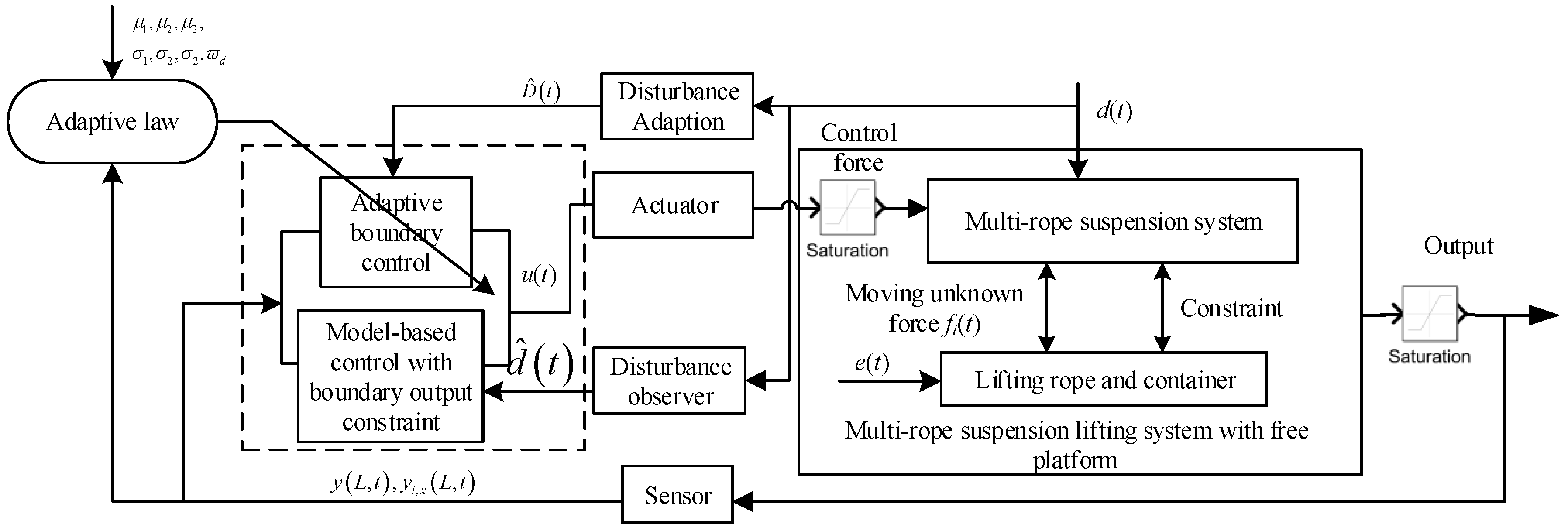
A boundary controller is proposed to reduce vibration of the MPSLS in transverse direction, and it guarantees that the position of the sinking platform remains in a small vicinity of origin. The dynamical model of the MPSLS is a nonhomogeneous and coupled PDEs-ODEs with infinite dimension. A model-based boundary control is based on the system energy and original PDEs-ODEs, which can directly deal with infinite dimensional system and avoid the spillover instability of the higher truncated modes. Then the model-based boundary control combining with adaptation laws is redesigned to reduce elastic vibration and regulate position of the sinking platform, while estimating unknown parameters. The control block diagram is shown in Figure 2.

3.1. Model-Based Boundary Control

Considering control input, subject to the magnitude constraint, the input saturation satisfies that
u ( t ) = { u max sgn ( u 0 ( t ) ) , | u 0 ( t ) | > u max u 0 ( t ) , | u 0 ( t ) | u max
where, u 0 ( t ) is the control command.
The control law based on precise model is given by
u 0 ( t ) = ( i = 1 n T i ( L ) y i , x ( L , t ) + k p m i = 1 n T i ( L ) T ¯ y i , x t ( L , t ) + m g ( β n y t ( L , t ) + α n 2 k p y ( L , t ) ) / B ( t ) ) + c y t ( L , t ) + { m u a ( t ) y ( L , t ) y t ( L , t ) D 2 [ y ( L , t ) ] 2 k 3 u a ( t ) } / B ( t ) k 1 u a ( t ) + k 2 ζ ( t ) sgn ( u a ( t ) ) d ¯
where, k 1 , k 2 , k 3 k p , α and β are positive constants; u a ( t ) is an auxiliary signal; B ( t ) and ζ ( t ) are auxiliary functions that handle the effect of the multiple constraints. u a ( t ) , B ( t ) and the time derivative of ζ ( t ) are given by
u a ( t ) = y t ( L , t ) + k p i = 1 n T i ( L ) T ¯ y i , x t ( L , t )
B ( t ) = ln 2 D 0 2 D 0 2 [ y ( L , t ) ] 2
ζ ˙ ( t ) = { k 0 ζ ( t ) u a Δ u + 0.5 Δ u 2 ζ ( t ) + Δ u , | ζ ( t ) | ζ 0 0 | ζ ( t ) | < ζ 0
where, Δ u = u ( t ) u 0 ( t ) , ln ( ) denotes the natural logarithm function, D 0 is a constraint on the sinking platform satisfying | y ( L , t ) | < D 0 . ζ 0 is a small positive design parameter. The proposed integral BLF B ( t ) guarantees that system state satisfies the output constraint.
A boundary disturbance observer is designed to compensate for d ( t ) , which is inevitable to the MPSLS. The basic method to the design observer is based on a tracking control algorithm, which corrects the disturbance estimation by estimating the error term d ˜ ( t ) = d ( t ) d ^ ( t ) , then we have
d ^ ˙ ( t ) = κ d ˜ ( t )
where, κ is a positive correction gain.
A new auxiliary function φ ( t ) is formalized as
φ ( t ) = d ^ ( t ) κ m y t ( L , t )
Combining the boundary condition of the sinking platform and Equation (29), we have
φ ˙ ( t ) = u a ( t ) B ( t ) κ ( φ ( t ) i = 1 n T i ( L ) y i , x ( L , t ) + u ( t ) + κ m y t ( L , t ) c y t ( L , t ) )
From Equations (13) and (30), the time derivatives of d ^ ( t ) is rewritten as
d ^ ˙ ( t ) = κ 1 d ˜ ( t ) + u a ( t ) B ( t )
Differentiating d ˜ ( t ) in Equation (25) with respect to time yields
d ˜ ˙ ( t ) = d ˙ d ^ ˙ ( t ) = d ˙ ( t ) ( κ 1 d ˜ ( t ) + u a ( t ) B ( t ) )
The control law Equation (25) is redesigned as
u 0 ( t ) = ( i = 1 n T i ( L ) y i , x ( L , t ) + k p m i = 1 n T i ( L ) T ¯ y i , x t ( L , t ) + m g ( β n y t ( L , t ) + α n 2 k p y ( L , t ) ) / B ( t ) ) + { m u a ( t ) y ( L , t ) y t ( L , t ) D 2 [ y ( L , t ) ] 2 k 3 u a ( t ) } / B ( t ) + c y t ( L , t ) k 1 u a ( t ) + k 2 ζ ( t ) d ^ ( t )
For the stability analysis, a Lyapunov candidate function (LCF) is defined as
V ( t ) = i = 1 n V 1 , i ( t ) + V 2 ( t ) + i = 1 n V 3 , i ( t ) + 1 2 [ d ˜ ( t ) ] 2
where
V 1 , i ( t ) = 1 2 n β k p ( ρ 0 L [ y i , t ( x , t ) ] 2 d x + 0 L T i ( x ) [ y i , x ( x , t ) ] 2 d x + k 4 [ y ( L , t ) ] 2 ) ,
V 2 ( t ) = 1 2 m u a 2 ( t ) B ( t ) + 1 2 [ ζ ( t ) ] 2 ,
V 3 , i ( t ) = γ ρ n 2 0 L ( L x ) y i , t ( x , t ) y i , x ( x , t ) d x + α ρ n 2 0 L y i , t ( x , t ) y i ( x , t ) d x ,
with k 4 , γ > 0 .
Then the following conclusions hold:
(a) The Equation (35) is a positive definite function as
0 λ 1 ( i = 1 n V 1 , i ( t ) + V 2 ( t ) + d ˜ ( t ) 2 ) V ( t ) λ 2 ( i = 1 n V 1 , i ( t ) + V 2 ( t ) + d ˜ ( t ) 2 )
where λ 1 , λ 2 > 0 (see Appendix A).
(b) The V ˙ ( t ) can be upper bounded with
V ˙ ( t ) λ V ( t ) + ψ
where, λ and ψ > 0 . Proof can be found in Appendix B.
The subsequent stability theorem will be proved with the above lemmas.
Theorem 1.
Combining Equations (2) and (20), the following inequality can be obtained as
n β k p T _ 2 L [ y i ( x , t ) ] 2 n β k p 2 0 L T i ( x ) [ y i , x ( x , t ) ] 2 d x i = 1 n V 1 i ( t ) 1 λ 1 V ( t ) L
1 2 [ ζ ( t ) ] 2 V 2 ( t ) 1 λ 1 V ( t ) L
Rearranging the above Equations (20) and (41), leads to
| y i ( x , t ) | 2 L n β k p T _ λ 1 ( V ( 0 ) e λ 3 t + ε λ 3 )
| ζ ( t ) | 2 λ 1 ( V ( 0 ) e λ t + ε λ )
As t , we further obtain
lim t | y i ( x , t ) | lim t 2 L n β k p T _ λ 1 ( V ( 0 ) e λ t + ε λ ) = 2 L ε n β k p T _ λ 1 λ ,
lim t | ζ ( t ) | lim t 2 λ 1 ( V ( 0 ) e λ t + ε λ ) = 2 ε λ 1 λ ,
Remark 4.
It is easily seen that the position of the sinking platform and the undesired vibration of the suspension rope can be diminished to an arbitrarily small value, when appropriately increasing the control gain k p satisfies the inequalities in Appendix B. However, the large control gain would also cause the high gain problem, even making the system unstable.
Remark 5.
The adaptation law Equation (32) is designed to estimate disturbance. We can conclude that the disturbance estimate error d ˜ ( t ) is bounded. Combining Equations (36) and (40), all system states of Equation (34) measured by sensors or calculations are uniformly bounded.

3.2. Robust Adaptive Boundary Control

When m and c are unknown, a robust adaptive boundary control is redesigned to asymptotically stabilize the system with multiple constraints, and to still estimate parametric uncertainties, which is given by
u 0 ( t ) = ϑ ( t ) m ^ ( t ) + { m ^ u a ( t ) y ( L , t ) y t ( L , t ) D 0 2 [ y ( L , t ) ] 2 k 3 u a ( t ) } / B ( t ) + c ^ ( t ) y t ( L , t ) k 1 u a ( t ) + k 2 ζ ( t ) + u i ( t )
where,
ϑ ( t ) = k p i = 1 n χ i y i , x t ( L , t ) g i = 1 n χ i y i , x ( L , t ) + g ( β n y t ( L , t ) + α n 2 k p y ( L , t ) ) / B ( t )
χ = [ χ 1 , χ 2 ] T = 1 D 1 + D 2 [ D 2 , D 1 ] T
Adaptation law of the parameter estimates m ^ ( t ) and c ^ ( t ) are defined as Equations (50) and (51). u i ( t ) is an auxiliary input function based on robust control strategy [33,34], as Equations (52) and (53).
m ^ ˙ ( t ) = μ 1 1 ϑ ( t ) u a ( t ) B ( t ) + μ 1 1 [ u a ( t ) ] 2 y ( L , t ) y t ( L , t ) D 0 2 [ y ( L , t ) ] 2 σ 1 μ 1 1 m ^ ( t )
c ^ ˙ ( t ) = μ 2 1 y t ( L , t ) u a ( t ) B ( t ) σ 2 μ 2 1 c ^ ( t )
u i ( t ) = [ D ^ ( t ) ] 2 u a ( t ) D ^ ( t ) | u a ( t ) | + ϖ d / B ( t )
D ^ ˙ ( t ) = μ 3 1 | u a ( t ) | B ( t ) σ 3 μ 3 1 D ^ ( t )
where, μ i , σ i and ϖ d are positive constants. D ^ ( t ) is the upper bounded estimation on d ¯ . Modification parameter σ i is introduced to improve the system robustness [35].
A new LCF is defined as
V a = i = 1 n V 1 , i ( t ) + V 2 ( t ) + i = 1 n V 3 , i ( t ) + V e ( t )
where, V 1 , i ( t ) , V 2 ( t ) and V 3 , i ( t ) are defined as Equations (36)–(38). V e ( t ) is given as
V e ( t ) = 1 2 ( μ 1 [ m ˜ ( t ) ] 2 + μ 2 [ c ˜ ( t ) ] 2 + μ 3 [ D ˜ ( t ) ] 2 )
Then the following Inequalities also hold:
(c) The Equation (54) is also a positive definite function as
0 λ 1 a ( i = 1 n V 1 , i ( t ) + V 2 ( t ) + [ m ˜ ( t ) ] 2 + [ c ˜ ( t ) ] 2 + [ D ˜ ( t ) ] 2 ) V a ( t ) λ 2 a ( i = 1 n V 1 , i ( t ) + V 2 ( t ) + [ m ˜ ( t ) ] 2 + [ c ˜ ( t ) ] 2 + [ D ˜ ( t ) ] 2 )
where λ 1 a and λ 2 a > 0 . Proof see Appendix C.
(d) The V ˙ a ( t ) can be upper bounded with
V ˙ a ( t ) λ a V a ( t ) + ε a
where, λ a , ε a > 0 . Proof can be found in Appendix D.
The subsequent stability theorem will be also proved with the above lemmas.
Theorem 2.
Combining Equations (2) and (20), the following inequality can be obtained as
n β k p T _ 2 L [ y i ( x , t ) ] 2 n β k p 2 0 L T i ( x ) [ y i , x ( x , t ) ] 2 d x i = 1 n V 1 i ( t ) 1 λ 1 a V a ( t ) L
1 2 [ ζ ( t ) ] 2 V 2 ( t ) 1 λ 1 a V a ( t ) L
Rearranging above Equations (20) and (41), we obtain
| y i ( x , t ) | 2 L n β k p T _ λ 1 a ( V a ( 0 ) e λ a t + ε a λ a ) ,
| ζ ( t ) | 2 λ 1 a ( V a ( 0 ) e λ a t + ε a λ a ) ,
As t , we further obtain
lim t | y i ( x , t ) | lim t 2 L n β k p T _ λ 1 a ( V a ( 0 ) e λ a t + ε a λ a ) = 2 L ε a n β k p T _ λ 1 a λ a ,
lim t | ζ ( t ) | lim t 2 λ 1 a ( V a ( 0 ) e λ a t + ε a λ a ) = 2 ε a λ 1 a λ a ,
Remark 6.
The adaptive boundary control law Equation (47) is designed to stabilize the system and to compensate for system uncertainties, and the boundedness of Equation (54) is guaranteed using Lyapunov’s direct method. According to LaSalle’s invariance principle, we can conclude that m ˜ ( t ) , c ˜ ( t ) and D ˜ ( t ) are also bounded and converged t [ 0 , ) . The MPSLS with multiple constraints has never been addressed. The proposed control is firstly designed for the MPSLS, with different and spatial distributed tensions, which jointly considers multiple constraints and the vibration degradation of the multi-rope system.

4. ADAMS Simulation and Numerical Calculation

Through the above stability analysis, both two control laws are effective methods to degrade vibration of the MPSLS. There is no analytical solution to the nonhomogeneous and coupled PDEs-ODEs with non-uniform tension, boundary disturbances, and multiple constraints, so the effectiveness of the proposed boundary control is illustrated by numerical simulation to obtain an approximation solution. The system parameters of the MPSLS are listed in Table 1.

4.1. ADAMS Simulation

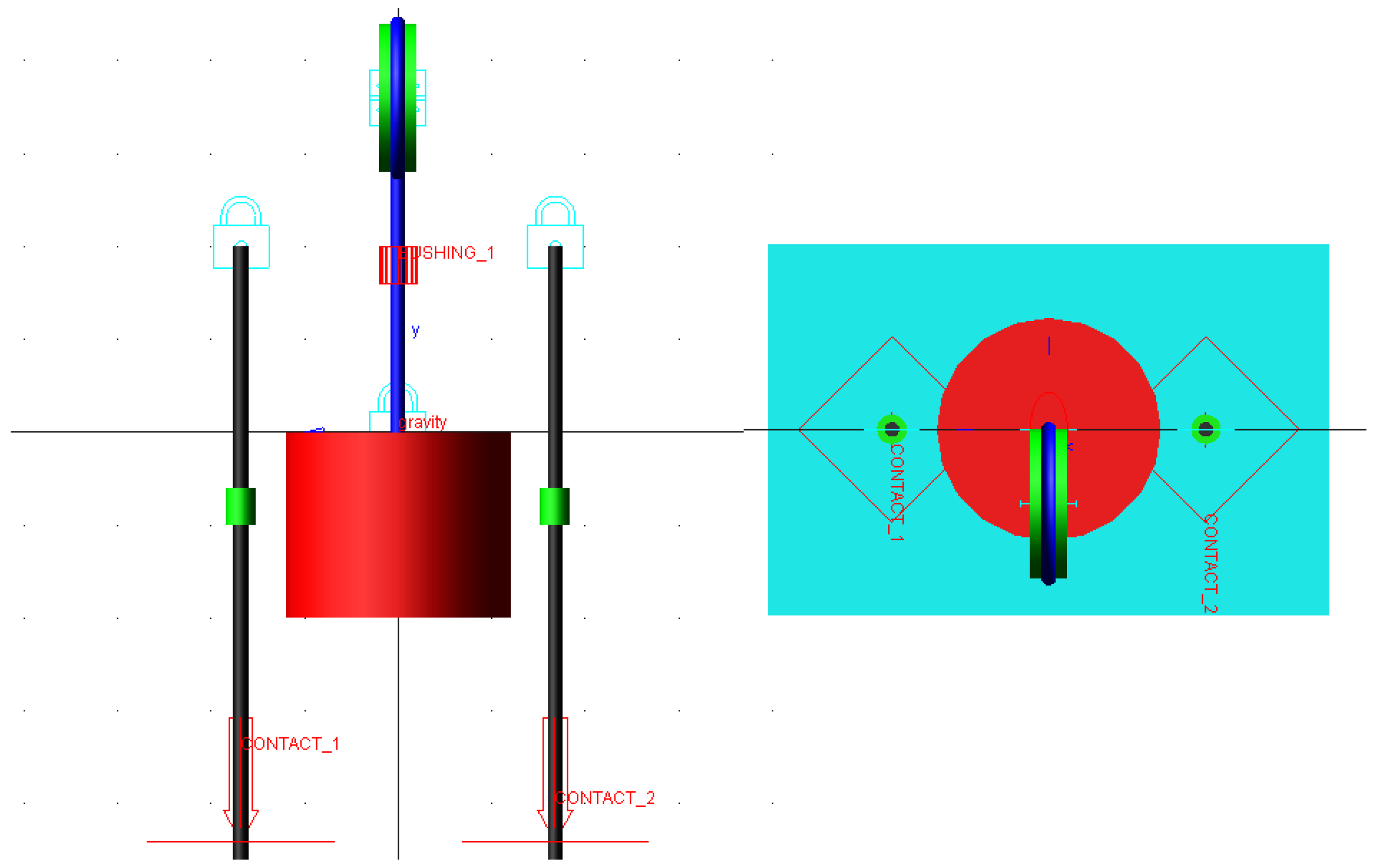
The ADAMS simulation is firstly verified through the theoretical model of the MPSLS in a simple case. Based on the multi-body dynamic theory, the suspension and lifting rope are discretized into a set of rigid bodies in the software ADAMS. Figure 3 shows a virtual prototype model of the MPSLS, without the bottom disturbance, and under zero initial conditions.
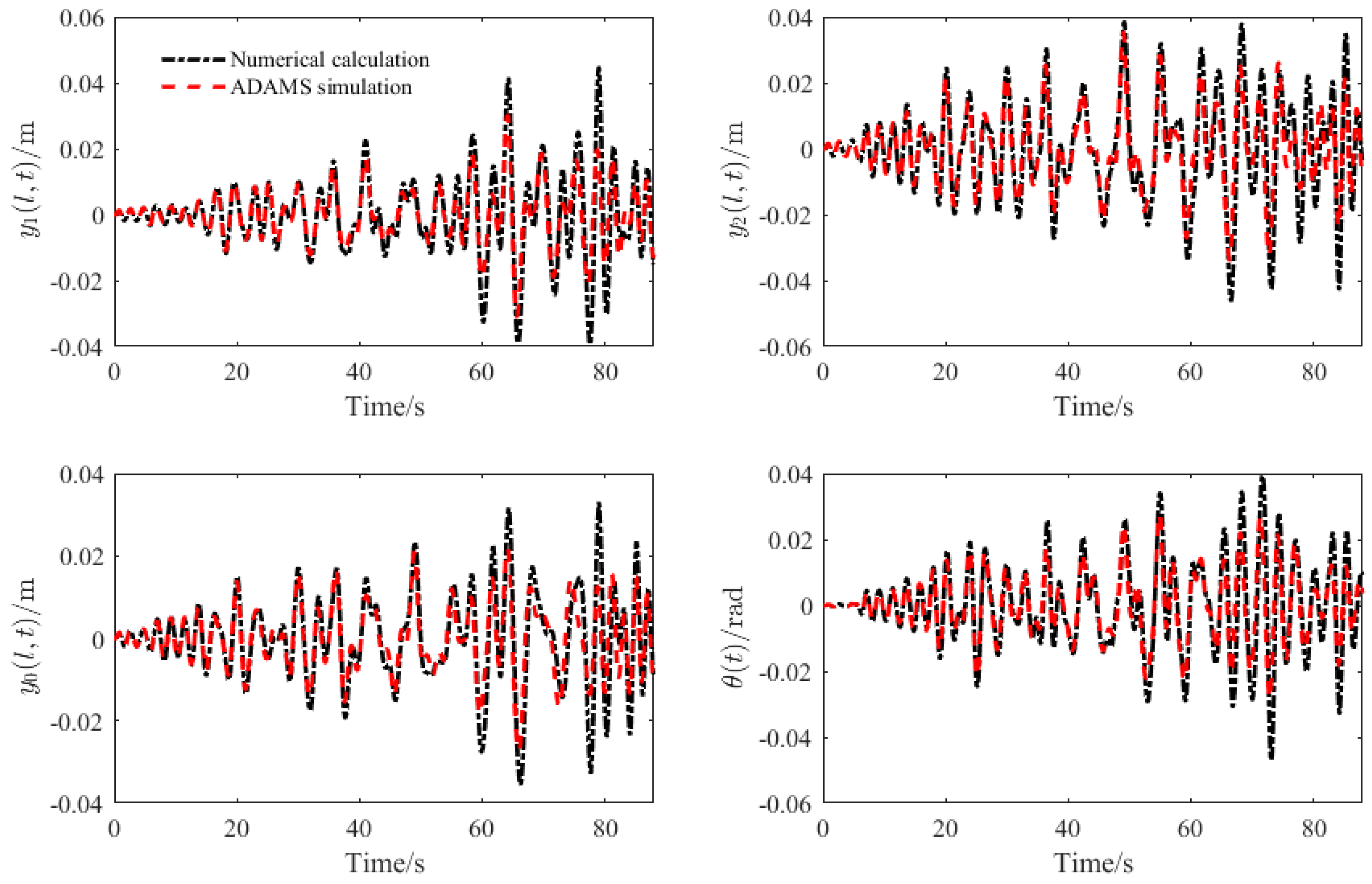
From Figure 4, the results of the modelling are consistent with the ADAMS result, which indicates that the modelling of the MPSLS is accurate and reasonable.

4.2. Different Cases

The following four cases were carried out in numerical results, to compare and validate the effect of the proposed control: (1) Without input; (2) The control law Equation (34); (3) The control law Equation (47); (4) The classical proportional–integral–derivative (PID) control [36]: u ( t ) = k s p y ( L , t ) k s i 0 t y ( L , τ ) d τ k s d y t ( L , t ) , with the parameters k s p = 10 4 , k s i = 10 2 and k s d = 1.2 × 10 3 . For the proposed controls, the appropriate parameters were chosen as follows: k 0 = 100 , k 1 = 10 7 , k 2 = 10 , k 3 = 1 , k 4 = 40 , k p = 30 , κ = 100 , α = β = 1 × 10 3 , σ 1 = 7.6 × 10 10 , σ 2 = 2.4 × 10 9 , σ 3 = 5.4 × 10 8 , μ 1 = 1.5 × 10 7 , μ 2 = 2.4 × 10 7 , μ 3 = 1.8 × 10 5 , d max = 1 × 10 3 N , ζ 0 = 0.05 , ϖ d = 0.02 , and u max = 9 × 10 2 N . The classical PID control has same saturation restriction on control input. The boundary disturbances were assumed as
d ( t ) = d max ( 0.1 + k = 1 3 2 k 1 10 sin ( ω k t ) ) N , e ( t ) = 0.02 sin ( π t ) m
The initial values were
y 0 ( x , 0 ) = 10 3 x m , y 0 , t ( x , 0 ) = 0   m / s , x [ 0 , l ( t ) ] y i ( x , 0 ) = 10 3 x m , y i , t ( x , 0 ) = 0   m / s , x [ 0 , L ] θ = 0   rad , θ ˙ = 0   rad / s .
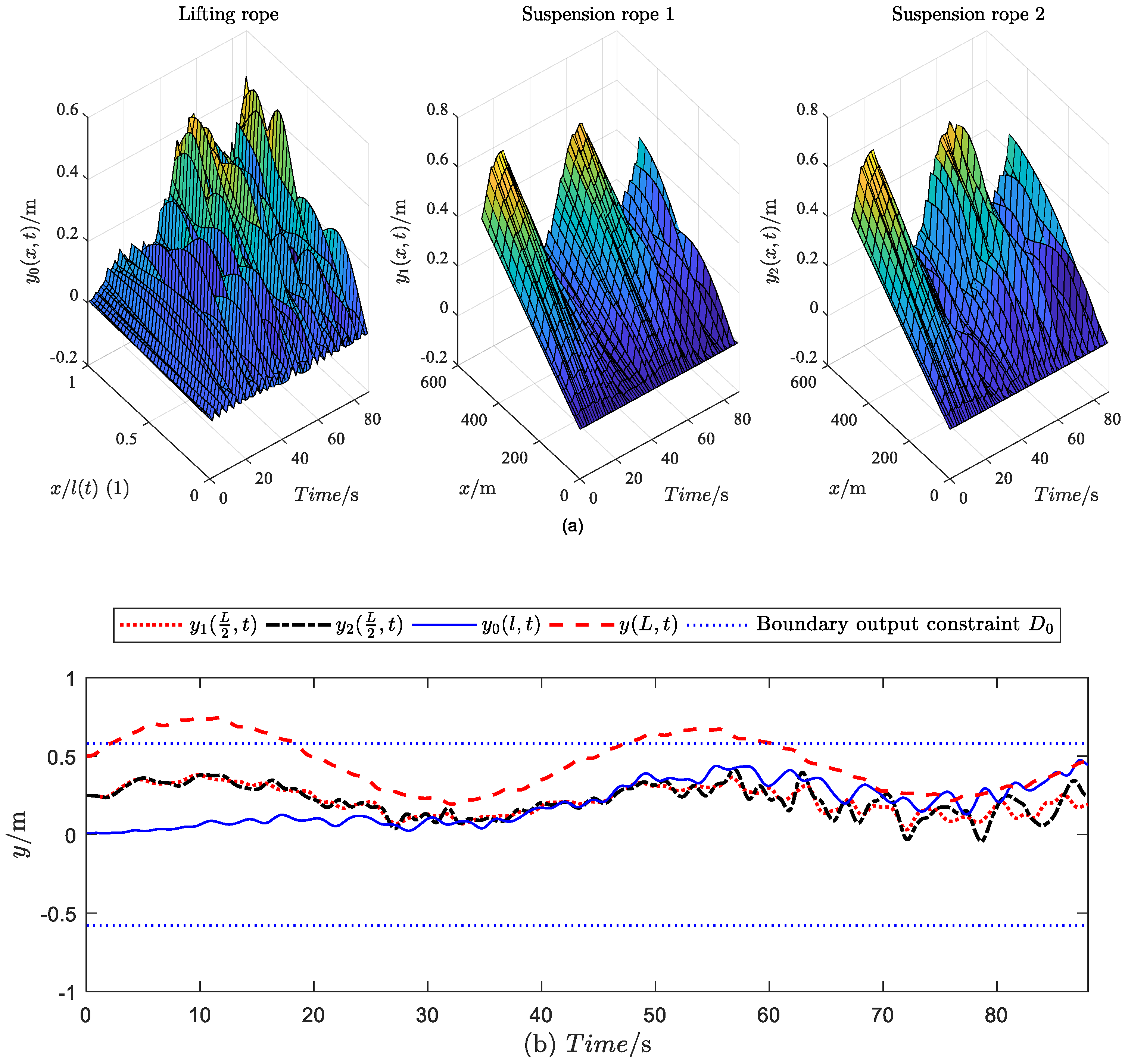
Without control input: The 3D transverse displacements of the two suspension ropes and the lifting rope without control are depicted in Figure 5a. The middle transverse displacements of the suspension ropes, the position of the lifting container, and the sinking platform, are shown in Figure 3b. It is obvious that the suspension ropes had a great transverse displacement from their equilibrium values, and the position of the sinking platform violated the boundary output constraint D 0 , under the external disturbance.
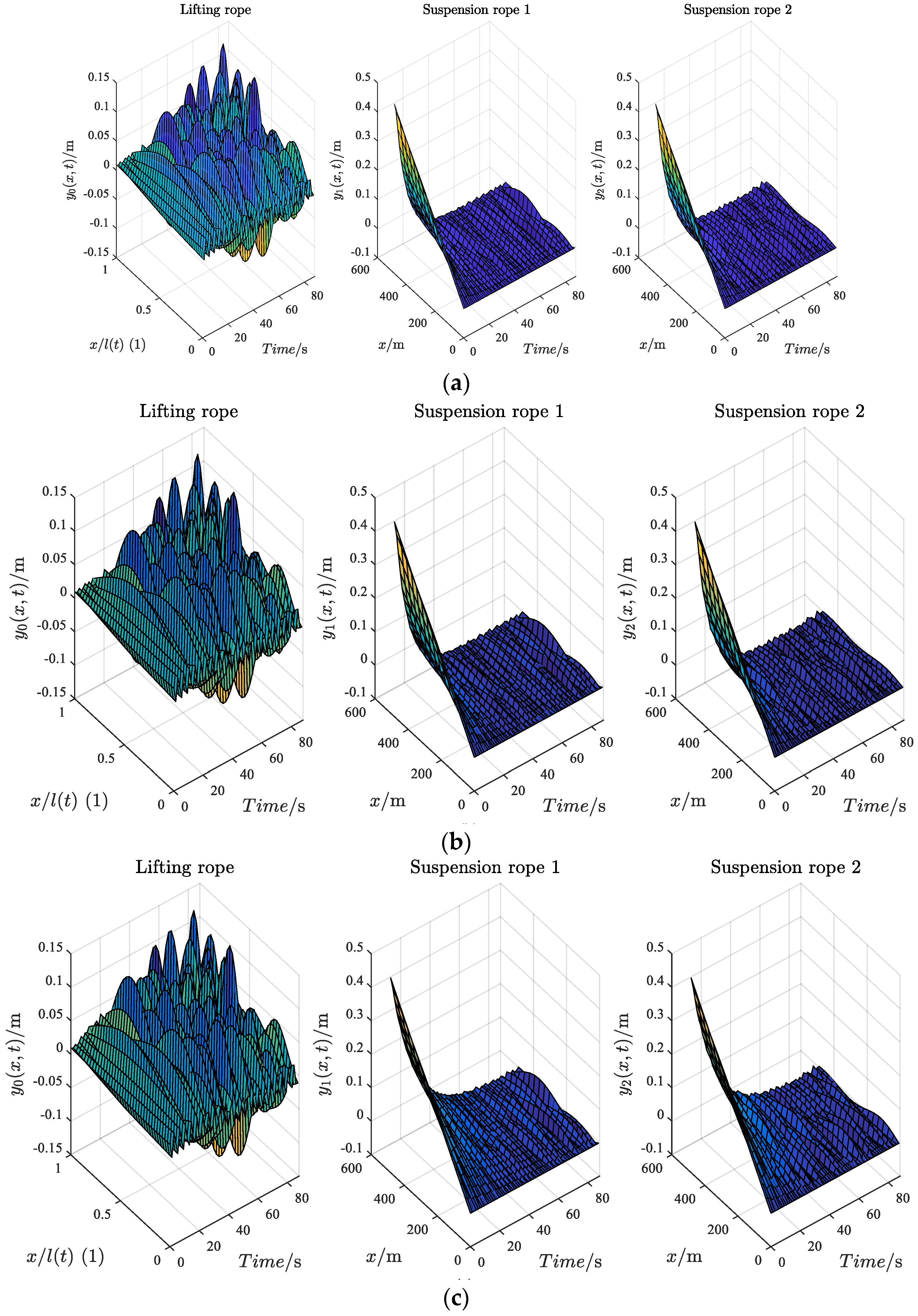
The 3D transverse displacements of the MPSLS, under proposed control, with external disturbance are displayed in Figure 6. The proposed boundary controls guarantee that the internal signals of the closed-loop system are bounded, and the displacement of the sinking platform y ( L , t ) eventually converges to zero as t tends to infinity, which satisfies the output constraint | y ( L , t ) | D 0 depicted in Figure 7. The responses of the sinking platform with classical PID control diminishes to a bounded neighborhood of zero after a much longer time in Figure 6c and Figure 7. Thus, the proposed control law shows better performance than the classical PID control.
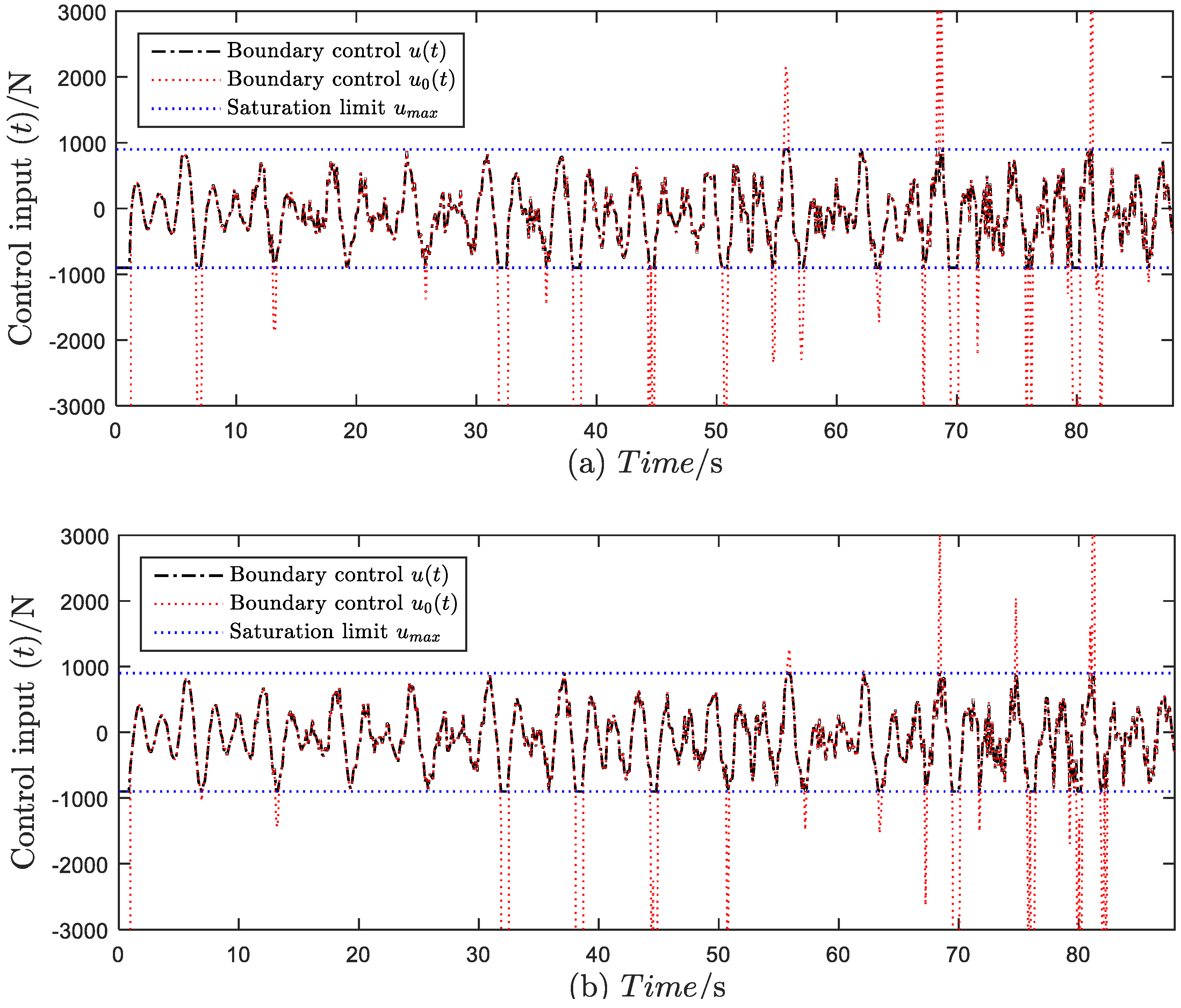
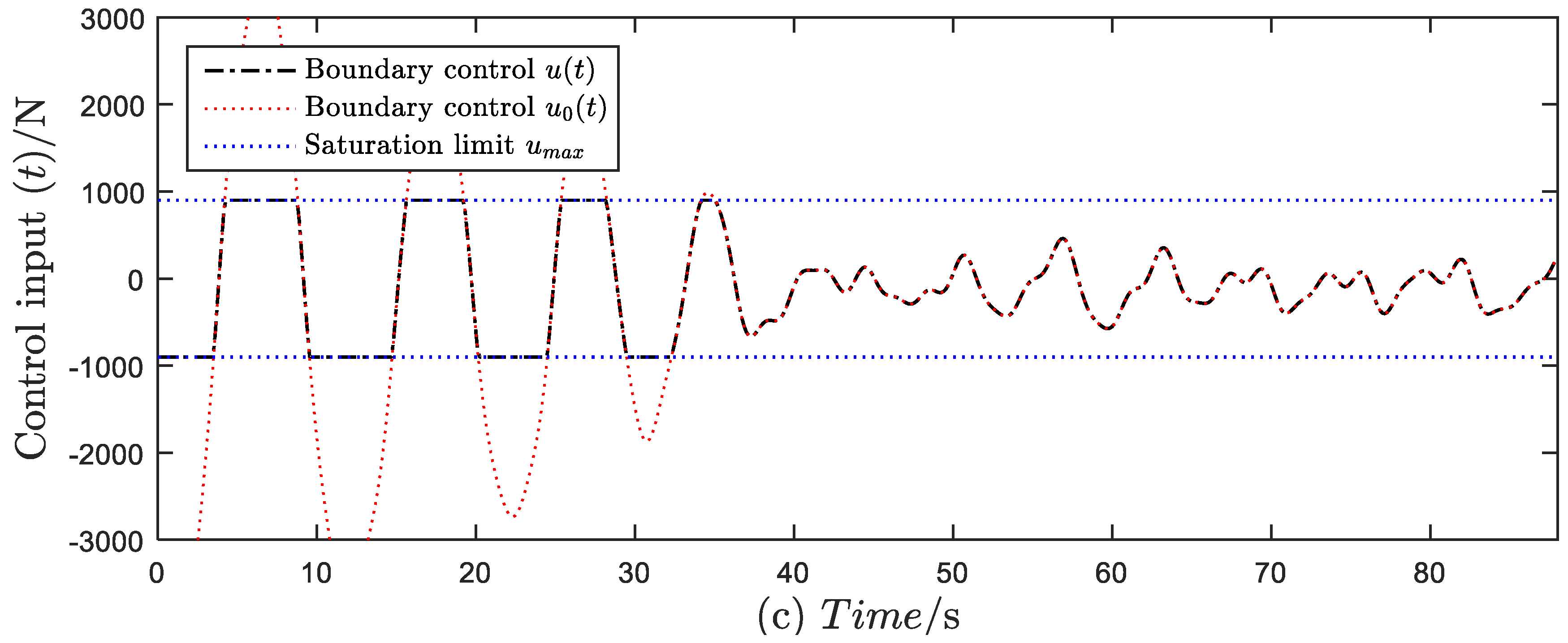
Control input of two control laws is displayed in Figure 8, where it is shown that control input u ( t ) does not exceed the saturation limit u max . In comparison, the design control inputs u 0 ( t ) exceed the saturation limit u max at certain times.
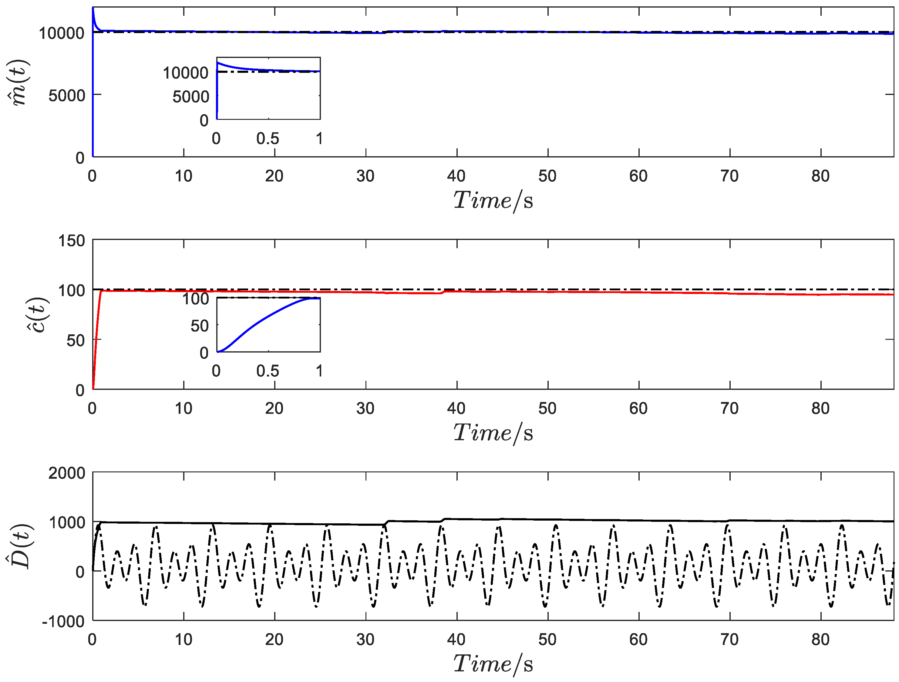
From Figure 9, the boundary disturbance estimate d ^ ( t ) converges to actual disturbance. From Figure 7 and Figure 9, the transverse displacement of the sinking platform under model-based boundary control Equation (34) converges faster than other laws, which indicates that the disturbance observer Equation (34) can compensate for an unknown disturbance more efficiently than a robust term Equation (47). Moreover, the parameter m ^ ( t ) , c ^ ( t ) and D ^ ( t ) also converge to the vicinity of the actual points shown in Figure 10. The adaptive control Equation (47) with a robust term still remains to stabilize the MPSLS, and it is a more extensive effective tool to tackle the problem of modeling and disturbance uncertainties.

5. Conclusions

In this paper, the modelling and control scheme of the MPSLS have been investigated in the presence of different and spatial distributed tensions, system parameter uncertainties, and multiple constraints, which is firstly verified by the ADAMS simulation. Based on the original PDEs-ODEs, two control laws were designed to both reduce vibration and regulate position of the MPSLS, with input saturation and output constraint. Based on the accurate model, an integral BLF and an auxiliary system were adopted to handle multiple constraints, and a disturbance observer was added to compensate for unknown boundary disturbance. Moreover, a robust adaptive boundary control combining with adaptation laws was redesigned to deal with unknown parameters for the MPSLS. The system stability and uniform boundedness under the proposed control laws were proved using Lyapunov synthesis. The transverse displacement of the MPSLS exponentially diminishes to a bounded neighborhood of origin, and the system states satisfy multiple constraints simultaneously.

Author Contributions

Methodology, N.W.; Providing modeling and control ideas, funding acquisition, G.C.; Investigation, N.W.; Data analysis, N.W. and L.W.; Writing—original draft, N.W.; Writing—review and editing, N.W. and L.Y.

Funding

This work is supported by the National Key Research and Development Program (2016YFC0600901), the National Natural Science Foundation of China (51475456) and Priority Academic Program Development (PAPD) of Jiangsu Higher Education Institutions.

Conflicts of Interest

The authors declare no conflict of interest.

Nomenclature

y i ( x , t ) Transverse displacement
a Arbitrary axial acceleration
v Arbitrary axial velocity
l The length of the lifting rope
L Total length of the suspension rope
J Inertia of the lifting container
m c Mass of the lifting container
T i ( x ) Tension of suspension rope
g The gravitational acceleration
E k ( t ) Kinetic energy
W ( t ) Virtual work
E p ( t ) Potential energy
d ( t ) Unknown boundary disturbance
u 0 ( t ) Control command
u max The saturation limit
ρ 1 Line density of the lifting rope
ρ Line density of the suspension rope
D i Geometric length
e ( t ) Transverse boundary disturbance
θ Rotation of the lifting container
t Time variable
x Space variable
T 0 ( x , t ) Tension in lifting rope
T i , 0 The bottom tension of the suspension rope
c c , c θ The damping coefficient
c The viscous damping of the sinking platform
δ ¯ ( x ) Dirac delta generalized function
f i ( t ) Unknown moving force
u ( t ) The control input
sgn ( · ) Signum function

Appendix A

Proof. Applying Lemmas 1 and 2 to Equation (28), the third term of the Lyapunov function candidate satisfies the following inequality
| V 3 , i ( t ) | ( ρ α + γ L n 2 0 L [ y i , t ( x , t ) ] 2 d x + ρ γ L + 4 α L 2 n 2 0 L [ y i , x ( x , t ) ] 2 d x + 2 ρ α L n 2 y 2 ( L , t ) ) α 1 V 1 , i ( t )
where, α 1 = 2 ρ max ( α + γ L β n 3 k p ρ , 4 α L 2 + γ L β n 3 k p T _ , 2 α L β n 3 k p k 4 ) . We have
α 1 i = 1 n V 1 , i ( t ) | i = 1 n V 3 , i ( t ) | α 1 i = 1 n V 1 , i ( t )
When α 1 satisfies 0 < α 1 < 1 , we have
0 λ 1 ( i = 1 n V 1 , i ( t ) + V 2 ( t ) + d ˜ ( t ) 2 ) V ( t ) λ 2 ( i = 1 n V 1 , i ( t ) + V 2 ( t ) + d ˜ ( t ) 2 )
where, λ 1 = min ( 1 α 1 , 1 2 ) , λ 2 = max ( 1 + α 1 , 1 ) .

Appendix B

Time derivative of Equation (35), we have
V ˙ ( t ) = i = 1 n V ˙ 1 , i ( t ) + V ˙ 2 ( t ) + i = 1 n V ˙ 3 , i ( t ) + d ˜ ( t ) d ˜ ˙ ( t ) 2
The V ˙ 1 , i ( t ) in the Equation (A4) is rewritten as
V ˙ 1 ( t ) = β n k p ( 0 L y i , t ( x , t ) ρ y i , t t ( x , t ) d x + 0 L T i ( x ) y i , x ( x , t ) y i , x t ( x , t ) d x + k 4 y ( L , t ) y t ( L , t ) )
Combining Equation (9) and Equation (A5), we obtain
V ˙ 1 ( t ) = β n k p i = 1 n ( T i ( L ) y i , t ( L , t ) y i , x ( L , t ) + 0 L y i , t ( f i ( t ) δ ¯ ( x l ) c i y i , t ) d x + k 4 y ( L , t ) y t ( L , t ) )
Using the boundary conditions of the sinking platform and integrating Equation (A6) by parts, we have
V ˙ 1 , i ( t ) = β n k p ( i = 1 n ( T i ( L ) y t ( L , t ) y i , x ( L , t ) + 0 L y i , t ( f i ( t ) δ ¯ ( x l ) c i y i , t ) d x ) + k 4 y ( L , t ) y t ( L , t ) ) ( β k p n 2 δ 1 i = 1 n 0 L f ¯ 2 δ ¯ ( x l ) d x + n 4 β k p δ 1 i = 1 n 0 L [ y i , t ( x , t ) ] 2 δ ¯ ( x l ) d x ) + β n k p ( i = 1 n ( T i ( L ) y t ( L , t ) y i , x ( L , t ) c i 0 L [ y i , t ( x , t ) ] 2 d x ) + k 4 y ( L , t ) y t ( L , t ) )
where, δ 1 > 0 .
Using the boundary conditions of the sinking platform and Equation (A7), we have
V ˙ 2 ( t ) ( B ( t ) k 1 + k 3 ) [ u a ( t ) ] 2 + u a ( t ) [ B ( t ) d ˜ ( t ) m g ( β n y t ( L , t ) + α n 2 k p y ( L , t ) ) ]
Since min { B ( t ) } = ln 2 D 0 2 D 0 2 = ln 2 , the above Equation (A8) can be rewritten as
V ˙ 2 ( t ) ( ln 2 k 1 + k 3 ) [ u a ( t ) ] 2 + u a ( t ) [ B ( t ) d ˜ ( t ) m g ( β n y t ( L , t ) + α n 2 k p y ( L , t ) ) ]
Using the governing equations of the suspension rope Equation (9) and Equation (19), integrating by part, we obtain
V ˙ 3 , i ( t ) ( γ L T i ( 0 ) 2 n 2 y i , x 2 ( 0 , t ) + 0 L ( γ T ¯ 2 n 2 + γ L δ 4 δ ¯ ( x l ) n 2 + γ c i L δ 5 n 2 ) [ y i , x ( x , t ) ] 2 d x + γ L n 2 δ 4 0 L f i 2 δ ¯ ( x l ) d x + γ c i L n 2 δ 5 0 L [ y i , t ( x , t ) ] 2 d x + γ ρ 2 n 2 0 L [ y i , t ( x , t ) ] 2 d x ) + ( α n 2 ( T i ( L ) y i ( L , t ) y i , x ( L , t ) T _ 2 0 L [ y i , x ( x , t ) ] 2 d x T _ 2 L y ( L , t ) 2 ) + α n 2 δ 2 0 L f i 2 δ ¯ ( x l ) d x + 0 L ( α δ 2 δ ¯ ( x l ) n 2 + α c i δ 3 n 2 ) L 2 [ y i , x ( x , t ) ] 2 d x + ( α c i n 2 δ 3 + α ρ n 2 ) 0 L [ y i , t ( x , t ) ] 2 d x )
where, δ i > 0 , i = 2 ~ 6 .
Applying Young’s Inequalities and Equation (33), the last term of the Equation (A4) is rewritten as
d ˜ ( t ) d ˜ ˙ ( t ) = d ˜ ( t ) ( d ˙ ( t ) κ d ˜ ( t ) u a ( t ) B ( t ) ) ( κ 1 δ 7 ) d ˜ 2 + δ 7 d ˙ 2 ( t ) d ˜ ( t ) u a ( t ) B ( t )
where, δ 7 > 0 .
Substituting Equations (A7)–(A11) into Equation (A4), it can be rearranged as the following form
V ˙ ( t ) ( ln 2 k 1 1 2 k 2 + k 3 ) [ u a ( t ) ] 2 i = 1 n ( c i β n k p n 4 β k p δ 1 α ρ n 2 α c i n 2 δ 3 γ c i L n 2 δ 5 γ ρ 2 n 2 ) 0 L [ y i , t ( x , t ) ] 2 d x i = 1 n 0 L ( α T _ 2 n 2 ( α δ 2 δ ¯ ( x l ) + α c i δ 3 ) L 2 n 2 ( γ T _ 2 n 2 + γ L δ 4 n 2 + γ c i L δ 5 n 2 ) ) [ y i , x ( x , t ) ] 2 d x ( β n M g | α M g β n 4 k p 2 k 1 | n 2 k p δ 6 ) [ y t ( L , t ) ] 2 ( α T _ 2 n 2 L | α M g β n 4 k p 2 k 1 | n 2 k p 1 δ 6 ) [ y ( L , t ) ] 2 ( γ L 2 n 2 α 2 n 2 ) i = 1 n T i ( 0 ) [ y i , x ( 0 , t ) ] 2 ( k 0 1 2 k 2 1 2 ) ζ 2 ( t ) ( κ 1 δ 7 ) d ˜ 2 + ( β k p n δ 1 + α n δ 2 + γ L n δ 4 ) 0 L f ¯ 2 δ ¯ ( x l ) d x + δ 7 d ˙ 2 ( t ) λ 3 ( i = 1 n V 1 , i ( t ) + V 2 ( t ) + d ˜ ( t ) 2 ) + ψ
where the constants k j ( j = 0 ~ 4 ) , k p , δ i ( i = 1 ~ 7 ) , κ , α , β and γ are selected to satisfy the following conditions:
0 < α 1 = 2 ρ max ( α + γ L β n 3 k p ρ , 4 α L 2 + γ L β n 3 k p T _ , 2 α L β n 3 k p k 4 ) < 1 τ 1 = ln 2 k 1 1 2 k 2 + k 3 > 0 τ 2 = c i β n k p n 4 β k p δ 1 α ρ n 2 α c i n 2 δ 3 γ c i L n 2 δ 5 γ ρ 2 n 2 > 0 τ 3 = α T _ 2 n 2 L 2 ( α δ 2 δ ¯ ( x l ) + α c i δ 3 ) n 2 ( γ T _ 2 n 2 + γ L δ 4 n 2 + γ c i L δ 5 n 2 ) > 0 τ 4 = β n M g | α M g β n 4 k p 2 k 1 | n 2 k p δ 6 > 0 τ 5 = α T _ 2 n 2 L | α M g β n 4 k p 2 k 1 | n 2 k p 1 δ 6 > 0 τ 6 = γ L 2 n 2 α 2 n 2 > 0 τ 7 = k 0 1 2 k 2 1 2 > 0 τ 8 = κ 1 δ 7 > 0 ε = ( β k p n δ 1 + α n δ 2 + γ L n δ 4 ) 0 L f ¯ 2 δ ¯ ( x l ) d x + δ 7 d ˙ 2 ( t ) λ 3 = min ( 2 τ 1 m , 2 τ 2 β n ρ k p , 2 τ 3 β n T _ k p , 2 τ 5 β n k 4 k p , 1 2 )
Combining Equations (A3) and (A12), we obtain
V ˙ ( t ) λ V ( t ) + ε
where, λ = λ 3 / λ 2 > 0 , and ε > 0 .

Appendix C

Proof. 
When α 1 satisfies 0 < α 1 < 1 , we obtain
0 λ 1 a ( i = 1 n V 1 , i ( t ) + V 2 ( t ) + [ m ˜ ( t ) ] 2 + [ c ˜ ( t ) ] 2 + [ D ˜ ( t ) ] 2 ) V a ( t ) λ 2 a ( i = 1 n V 1 , i ( t ) + V 2 ( t ) + [ m ˜ ( t ) ] 2 + [ c ˜ ( t ) ] 2 + [ D ˜ ( t ) ] 2 )
where, λ 1 a = min ( 1 α 1 , 1 2 μ 1 , 1 2 μ 2 , 1 2 μ 3 ) > 0 , λ 2 a = max ( 1 + α 1 , 1 2 μ 1 , 1 2 μ 2 , 1 2 μ 3 ) > 1 .  ☐

Appendix D

Time derivative of Equation (54), we have
V ˙ a = i = 1 n V ˙ 1 , i ( t ) + V ˙ 2 ( t ) + i = 1 n V ˙ 3 , i ( t ) + V ˙ e ( t )
Substituting the boundary condition of the sinking platform Equation (13) and using Equation (19), the second term of the Equation (A15) can be translated into following form
V ˙ 2 ( t ) u a ( t ) m u ˙ a ( t ) B ( t ) + 1 2 m [ u a ( t ) ] 2 B ˙ ( t ) + ζ ( t ) ζ ˙ ( t ) ( m ˜ u a 2 ( t ) y ( L , t ) y t ( L , t ) D 0 2 [ y ( L , t ) ] 2 k 3 u a 2 ( t ) k 1 u a 2 ( t ) B ( t ) + u a ( t ) ( ϑ ( t ) M ˜ c ˜ ( t ) y t ( L , t ) ) B ( t ) ) ( k 0 1 2 k 2 1 2 ) ζ 2 ( t ) + 1 2 k 2 u a 2 ( t ) + u a ( t ) ( u i ( t ) + d ( t ) ) B ( t )
Substituting the auxiliary input function Equation (52) into the third term of Equation (A16), we have
u a ( t ) ( u i ( t ) + d ( t ) ) B ( t ) = ( D ^ 2 ( t ) | u a ( t ) | 2 D ^ ( t ) | u a ( t ) | + ϖ d / B ( t ) + d ( t ) u a ( t ) ) B ( t )
Using the inequality ϱ | ϱ | , ϱ and | d ( t ) | d ¯ , we get
u a ( t ) ( u i ( t ) + d ( t ) ) B ( t ) = ( D ^ ( t ) 2 | u a ( t ) | 2 D ^ ( t ) | u a ( t ) | + ϖ d / B ( t ) + d ( t ) u a ( t ) ) B ( t ) ( D ^ ( t ) 2 | u a ( t ) | 2 + d ¯ | u a ( t ) | ( D ^ ( t ) | u a ( t ) | + ϖ d / B ( t ) ) D ^ ( t ) | u a ( t ) | + ϖ d / B ( t ) ) B ( t )
Since D ˜ ( t ) = D ^ ( t ) d ¯ and
D ^ ( t ) 2 | u a ( t ) | 2 + d ¯ | u a ( t ) | ( D ^ ( t ) | u a ( t ) | + ϖ d / B ( t ) ) D ^ ( t ) | u a ( t ) | + ϖ d / B ( t ) ( ϖ d / B ( t ) ) 2 D ^ ( t ) | u a ( t ) | + ϖ d / B ( t ) + D ^ ( t ) 2 | u a ( t ) | 2 + d ¯ | u a ( t ) | ( D ^ ( t ) | u a ( t ) | + ϖ d / B ( t ) ) D ^ ( t ) | u a ( t ) | + ϖ d / B ( t ) ,
we obtain
( ϖ d / B ( t ) ) 2 D ^ ( t ) 2 | u a ( t ) | 2 + d ¯ | u a ( t ) | ( D ^ ( t ) | u a ( t ) | + ϖ d / B ( t ) ) D ^ ( t ) | u a ( t ) | + ϖ d / B ( t ) B ( t ) ( ϖ d / B ( t ) D ^ ( t ) | u a ( t ) | + d ¯ | u a ( t ) | ) B ( t ) = ϖ d ( D ^ ( t ) d ¯ ) | u a ( t ) | B ( t ) = ϖ d D ˜ ( t ) | u a ( t ) | B ( t )
Applying Young’s Inequality a b 1 2 ( a 2 + b 2 ) , we have
V ˙ e ( t ) [ m ˜ ( t ) ϑ ( t ) c ˜ ( t ) y t ( L , t ) ] u a ( t ) B ( t ) m ˜ u a ( t ) 2 y ( L , t ) y t ( L , t ) D 0 2 [ y ( L , t ) ] 2 + σ 1 m ˜ ( t ) m ^ ( t ) + σ 2 c ˜ ( t ) c ^ ( t ) + 1 2 σ 3 ( D 2 D ˜ ( t ) 2 ) + D ˜ ( t ) | u a ( t ) | B ( t ) [ m ˜ ( t ) ϑ ( t ) c ˜ ( t ) y t ( L , t ) ] u a ( t ) B ( t ) m ˜ u a 2 ( t ) y ( L , t ) y t ( L , t ) D 0 2 [ y ( L , t ) ] 2 1 2 σ 1 m ˜ 2 ( t ) + 1 2 σ 1 m 2 1 2 σ 2 c ˜ 2 ( t ) + 1 2 σ 2 c 2 + 1 2 σ 3 ( D 2 D ˜ ( t ) 2 ) + D ˜ ( t ) | u a ( t ) | B ( t )
Substituting Equations (A7), (A10), (A16), and (A21) into Equation (A15), we obtain
V ˙ ( t ) ( ln 2 k 1 1 2 k 2 + k 3 ) [ u a ( t ) ] 2 i = 1 n ( c i β n k p n 4 β k p δ 1 α ρ n 2 α c i n 2 δ 3 γ c i L n 2 δ 5 γ ρ 2 n 2 ) 0 L [ y i , t ( x , t ) ] 2 d x i = 1 n 0 L ( α T _ 2 n 2 ( α δ 2 δ ¯ ( x l ) + α c i δ 3 ) L 2 n 2 ( γ T _ 2 n 2 + γ L δ 4 n 2 + γ c i L δ 5 n 2 ) ) [ y i , x ( x , t ) ] 2 d x ( β n M g | α M g β n 4 k p 2 k 1 | n 2 k p δ 6 ) [ y t ( L , t ) ] 2 ( α T _ 2 n 2 L | α M g β n 4 k p 2 k 1 | n 2 k p 1 δ 6 ) [ y ( L , t ) ] 2 ( γ L 2 n 2 α 2 n 2 ) i = 1 n T i ( 0 ) [ y i , x ( 0 , t ) ] 2 ( k 0 1 2 k 2 1 2 ) ζ 2 ( t ) 1 2 ( σ 1 m ˜ 2 ( t ) + σ 2 c ˜ 2 ( t ) + σ 3 D ˜ ( t ) 2 ) + ( β k p n δ 1 + α n δ 2 + γ L n δ 4 ) 0 L f ¯ 2 δ ¯ ( x l ) d x + ϖ d + 1 2 ( σ 1 m 2 + σ 2 c 2 + σ 3 D 2 ) λ 3 ( i = 1 n V 1 , i ( t ) + V 2 ( t ) + V e ( t ) ) + ψ
where the constants k j ( j = 0 ~ 4 ) , k p , δ i ( i = 1 ~ 6 ) , α , β γ σ i , μ i and ϖ d are selected to satisfy the following conditions:
0 < α 1 = 2 ρ max ( α + γ L β n 3 k p ρ , 4 α L 2 + γ L β n 3 k p T _ , 2 α L β n 3 k p k 4 ) < 1 τ 1 = ln 2 k 1 1 2 k 2 + k 3 > 0 τ 2 = c i β n k p n 4 β k p δ 1 α ρ n 2 α c i n 2 δ 3 γ c i L n 2 δ 5 γ ρ 2 n 2 > 0 τ 3 = α T _ 2 n 2 L 2 ( α δ 2 δ ¯ ( x l ) + α c i δ 3 ) n 2 ( γ T _ 2 n 2 + γ L δ 4 n 2 + γ c i L δ 5 n 2 ) > 0 τ 4 = β n M g | α M g β n 4 k p 2 k 4 | n 2 k p δ 6 > 0 τ 5 = α T _ 2 n 2 L | α M g β n 4 k p 2 k 4 | n 2 k p 1 δ 6 > 0 τ 6 = γ L 2 n 2 α 2 n 2 > 0 τ 7 = k 0 1 2 k 2 1 2 > 0 ε a = ( β k p n δ 1 + α n δ 2 + γ L n δ 4 ) 0 L f ¯ 2 δ ¯ ( x l ) d x + ϖ d + 1 2 ( σ 1 m 2 + σ 2 c 2 + σ 3 D 2 ) λ 3 a = min ( 2 τ 1 m , 2 τ 2 β n ρ k p , 2 τ 3 β n T _ k p , 2 τ 5 β n k 4 k p , σ 1 2 , σ 2 2 , σ 3 2 )
Combining Equations (A14) and(A22), we have
V ˙ ( t ) λ a V ( t ) + ε a
where, λ a = λ 3 a / λ 2 a > 0 and ε a > 0 .

References

  1. Michael, N.; Fink, J.; Kumar, V. Cooperative manipulation and transportation with aerial robots. Auton. Robot. 2011, 30, 73–86. [Google Scholar] [CrossRef]
  2. Mao, Y.; Jin, X.; Gera Dutta, G.; Scholz, J.P.; Agrawal, S.K. Human movement training with a cable Driven ARm EXoskeleton (CAREX). IEEE Trans. Neural Syst. Rehabil. Eng. 2015, 23, 84–92. [Google Scholar] [CrossRef] [PubMed]
  3. Andréa-Novel, B.D.; Coron, J.M. Exponential stabilization of an overhead crane with flexible cable via a back-stepping approach. Automatica 2000, 36, 587–593. [Google Scholar] [CrossRef]
  4. Elbadawy, A.A.; Shehata, M.M.G. Anti-sway control of marine cranes under the disturbance of a parallel manipulator. Nonlinear Dyn. 2015, 82, 1–20. [Google Scholar] [CrossRef]
  5. Do, K.D.; Pan, J. Boundary control of three-dimensional inextensible marine risers. J. Sound Vib. 2009, 327, 299–321. [Google Scholar] [CrossRef]
  6. Fung, R.F.; Liao, C.C. Application of variable structure control in the nonlinear string system. Int. J. Mech. Sci. 1995, 37, 985–993. [Google Scholar] [CrossRef]
  7. Pi, Y.; Ouyang, H. Vibration control of beams subjected to a moving mass using a successively combined control method. Appl. Math. Model. 2016, 40, 4002–4015. [Google Scholar] [CrossRef]
  8. He, W.; Yan, Z.; Sun, C.; Chenm, Y. Adaptive neural network control of a flapping wing micro aerial vehicle with disturbance observer. IEEE Trans. Cybern. 2017, 47, 3452–3465. [Google Scholar] [CrossRef] [PubMed]
  9. He, W.; Huang, H.; Ge, S.S. Adaptive neural network control of a robotic manipulator with time-varying output constraints. IEEE Trans. Cybern. 2017, 47, 3136–3147. [Google Scholar] [CrossRef] [PubMed]
  10. Qu, Z. Robust and adaptive boundary control of a stretched string on a moving transporter. IEEE Trans Automat. Control 2001, 46, 470–476. [Google Scholar]
  11. Baz, A. Dynamic boundary control of beams using active constrained layer damping. Mech. Syst. Signal. Process. 1997, 11, 811–825. [Google Scholar] [CrossRef]
  12. Meirovitch, L.; Kwak, M. convergence of the classical rayleigh-ritz method and the finite element method. AIAA J. 1990, 28, 1509–1516. [Google Scholar] [CrossRef]
  13. Balas, M.J. Active control of flexible systems. J. Optim. Theor. Appl. 1978, 25, 415–436. [Google Scholar] [CrossRef]
  14. He, W.; Ge, S.S. Robust adaptive boundary control of a vibrating string under unknown time-varying disturbance. IEEE Trans. Control Syst. Technol. 2011, 20, 48–58. [Google Scholar] [CrossRef]
  15. How, B.V.E.; Ge, S.S.; Choo, Y.S. Active control of flexible marine risers. J. Sound Vib. 2009, 320, 758–776. [Google Scholar] [CrossRef]
  16. Yang, K.; Hong, K.; Matsuno, F. Robust adaptive boundary control of an axially moving string under a spatiotemporally varying tension. J. Sound Vib. 2004, 273, 1007–1029. [Google Scholar] [CrossRef]
  17. Guo, B.; Jin, F. The active disturbance rejection and sliding mode control approach to the stabilization of the Euler-Bernoulli beam equation with boundary input disturbance. Automatica 2013, 49, 2911–2918. [Google Scholar] [CrossRef]
  18. Azinheira, J.R.; Moutinho, A. Hover control of an UAV with backstepping design including input saturations. IEEE Trans. Control Syst. Technol. 2008, 16, 517–526. [Google Scholar] [CrossRef]
  19. Zhong, Y.S. Globally stable adaptive system design for minimum phase SISO plants with input saturation. Automatica 2005, 41, 1539–1547. [Google Scholar] [CrossRef]
  20. Zhang, T.P.; Ge, S.S. Adaptive dynamic surface control of nonlinear systems with unknown dead zone in pure feedback form. Automatica 2008, 44, 1895–1903. [Google Scholar] [CrossRef]
  21. Tee, K.P.; Ren, B.; Ge, S.S. Control of nonlinear systems with time-varying output constraints. Automatica 2011, 47, 2511–2516. [Google Scholar] [CrossRef]
  22. He, W.; Ma, T. Adaptive neural network control of a vessel with output constraints using the asymmetric barrier lyapunov function. IFAC Proc. Vol. 2013, 46, 246–251. [Google Scholar] [CrossRef]
  23. Liu, Z.; Liu, J.; He, W. Vibration control of a flexible aerial refuelling hose with input saturation. Int. J. Syst. Sci. 2017, 48, 971–983. [Google Scholar] [CrossRef]
  24. Zhou, J.; Wen, C. Adaptive Backstepping Control of Uncertain Systems Nonsmooth Nonlinearities, Interactions or Time-Variations; Springer: Berlin, Germany, 2008; ISBN 3540778063. [Google Scholar]
  25. He, W.; Yan, Z.; Sun, Y.; Ou, Y.; Sun, C. Neural-learning-based control for a constrained robotic manipulator with flexible joints. IEEE Trans. Neural Netw. Learn. Syst. 2018, 1–11. [Google Scholar] [CrossRef] [PubMed]
  26. He, W.; Dong, Y. Adaptive fuzzy neural network control for a constrained robot using impedance learning. IEEE Trans. Neural Netw. Learn. Syst. 2018, 29, 1174–1186. [Google Scholar] [CrossRef] [PubMed]
  27. He, W.; He, X.; Ge, S.S. Modeling and vibration control of a coupled vessel-mooring-riser system. IEEE/ASME Trans. Mechatron. 2015, 20, 2832–2840. [Google Scholar] [CrossRef]
  28. He, W.; Zhang, S.; Ge, S.S. Robust adaptive control of a thruster assisted position mooring system. Automatica 2014, 50, 1843–1851. [Google Scholar] [CrossRef]
  29. Cai, X.; Krstic, M. Nonlinear stabilization through wave PDE dynamics with a moving uncontrolled boundary. Automatica 2016, 68, 27–38. [Google Scholar] [CrossRef]
  30. Krstic, M. Boundary Control. of PDEs: A Course on Backstepping Designs; Society for Industrial and Applied Mathematics: Philadelphia, PA, USA, 2008; ISBN 9780898716504. [Google Scholar]
  31. Rahn, C.D. Mechatronic Control of Distributed Noise and Vibration; Springer: Berlin/Heidelberg, Germany, 2001; ISBN 978-3-642-07536-0. [Google Scholar]
  32. Queiroz, M.S.D.; Dawson, D.M.; Nagarkatti, S.P.; Zhang, F. Lyapunov-Based Control. of Mechanical Systems; Birkhäuser: Boston, NY, USA, 2000; ISBN 978-1-4612-7108-6. [Google Scholar]
  33. Yang, K.J.; Hong, K.S.; Matsuno, F. Energy-based control of axially translating beams: Varying tension, varying speed, and disturbance adaptation. IEEE Trans. Control Syst. Technol. 2005, 13, 1045–1054. [Google Scholar] [CrossRef]
  34. Yang, K.; Hong, K.; Matsuno, F. Robust adaptive control of a cantilevered flexible structure with spatiotemporally varying coefficients and bounded disturbance. JSME Int J. Ser. C 2005, 47, 812–822. [Google Scholar] [CrossRef]
  35. Ioannou, P.A.; Sun, J. Robust Adaptive Control; Prentice-Hall: Saddle River, NJ, USA, 1996; ISBN 0134391004. [Google Scholar]
  36. Yang, D.-H.; Kim, K.-Y.; Kwak, M.K.; Lee, S. Dynamic modeling and experiments on the coupled vibrations of building and elevator ropes. J. Sound Vib. 2017, 390, 164–191. [Google Scholar] [CrossRef]
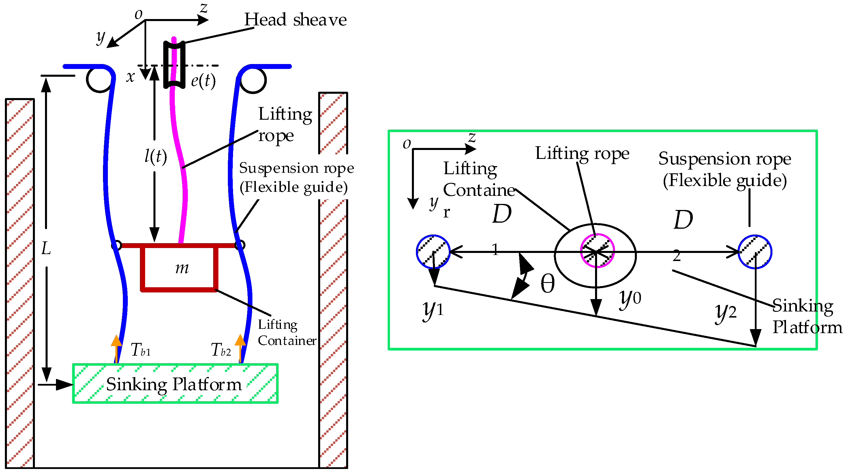
Figure 1. A multi-rope parallel suspension lifting system (MPSLS).
Symmetry 10 00412 g001
Figure 2. Control block diagram.
Symmetry 10 00412 g002
Figure 3. ADAMS model.
Symmetry 10 00412 g003
Figure 4. Simulation results: ADAMS simulation in red line and Numerical calculation in black line.
Symmetry 10 00412 g004
Figure 5. Displacement of the system without input: (a) 3D transverse displacement; (b) Midpoint and boundary displacements of the system.
Symmetry 10 00412 g005
Figure 6. 3D transverse displacement: (a) Control law Equation (34); (b) Control law Equation (47); (c) Control law PID.
Symmetry 10 00412 g006
Figure 7. Transverse displacement of the sinking platform with different cases: (a) The displacement of the sinking platform; (b) The displacement of the lifting container.
Symmetry 10 00412 g007
Figure 8. Control input: (a) Control law Equation (34); (b) Control law Equation (47); (c) Control law PID.
Symmetry 10 00412 g008aSymmetry 10 00412 g008b
Figure 9. The boundary disturbance estimate under the model-based control Equation (47).
Symmetry 10 00412 g009
Figure 10. Parameter estimations with adaptive boundary control Equation (47).
Symmetry 10 00412 g010
Table 1. Key parameters.
ParameterDescriptionValue
L Total length of the suspension rope500 m
l ( 0 ) Initial length of lifting rope10 m
m c Mass of the lifting container500 kg
m Mass of the sinking platform10 t
J Inertia of the lifting container 70 kg m2
ρ 1 , ρ Mass per unit length of the rope2 kg/m, 1.5 kg/m
a max Maximum acceleration of the lifting rope0.75 m/s2
v max Maximum velocity of the lifting rope6 m/s
t f Total duration time88 s
c , c c , c i , c θ Damping coefficient 100 , 0.001 , 0.001 , 0.005   Nsm
D 1 , D 2 Geometrical distance0.54 m, 0.66 m
D 0 Constrained positive constant0.58 m