Article

Intersection Traffic Prediction Using Decision Tree Models

1
School of Computer Science, Guangzhou University, Guangzhou 510006, China
2
School of Information Technology, Deakin University, Geelong, VIC 3220, Australia
3
School of Mathematics and Computing Science, Guilin University of Electronic Technology, Guilin 541004, China
4
School of Software and Electrical Engineering, Swinburne University of Technology, Hawthorn, VIC 3122, Australia
*
Author to whom correspondence should be addressed.
Current address: Guangzhou Higher Education Mega Center, 230 Wai Huan Xi Road, Guangzhou 510006, China.
Symmetry 2018, 10(9), 386; https://doi.org/10.3390/sym10090386
Submission received: 19 August 2018 / Revised: 2 September 2018 / Accepted: 3 September 2018 / Published: 7 September 2018

Abstract

:
Traffic prediction is a critical task for intelligent transportation systems (ITS). Prediction at intersections is challenging as it involves various participants, such as vehicles, cyclists, and pedestrians. In this paper, we propose a novel approach for the accurate intersection traffic prediction by introducing extra data sources other than road traffic volume data into the prediction model. In particular, we take advantage of the data collected from the reports of road accidents and roadworks happening near the intersections. In addition, we investigate two types of learning schemes, namely batch learning and online learning. Three popular ensemble decision tree models are used in the batch learning scheme, including Gradient Boosting Regression Trees (GBRT), Random Forest (RF) and Extreme Gradient Boosting Trees (XGBoost), while the Fast Incremental Model Trees with Drift Detection (FIMT-DD) model is adopted for the online learning scheme. The proposed approach is evaluated using public data sets released by the Victorian Government of Australia. The results indicate that the accuracy of intersection traffic prediction can be improved by incorporating nearby accidents and roadworks information.

1. Introduction

In recent years, intelligent transportation systems (ITS) have developed around the world as part of smart cities, integrating various technologies like cloud computing, the Internet of Things, sensors, artificial intelligence, geographical information, and social networks [1,2,3,4,5,6,7,8]. The innovative services provided by ITS can improve transportation mobility and safety by making road users better informed and more coordinated, which helps in addressing the transportation issues caused by the significant increase in city traffic in the past few decades.
Traffic prediction is one of the key tasks of ITS. It provides essential information to road users and traffic management agencies to allow better decision making. It also helps to improve transport network planning to reduce common problems, such as road accidents, traffic congestion, and air pollution [9]. The most complex part of the transport network comprises intersections [10], where various parties, including vehicles, cyclists, and pedestrians, interact with each other. It is reported that 40% of car crashes in the United States occurred at intersections in 2008 [11]. Therefore, accurate traffic prediction at intersections is critical for maintaining the mobility and safety of transportation.
A significant number of studies have investigated the traffic prediction problem with the aim of increasing the accuracy and efficiency of predictions. There are two key challenges in the application of traffic prediction, especially at intersections. First, traffic prediction is a dynamic, nonlinear problem [12]. A distinguishing feature of traffic flow is the presence of recurrent patterns over time which is useful for traffic prediction models. However, there are also nonrecurring events, such as accidents or roadworks, which could significantly affect the accuracy of prediction. Therefore, incorporating real-time spatio-temporal information related to the nonrecurring events could aid in accurate traffic prediction. These events, along with the time and space variation patterns, require a nonlinear model [13]. There are also other factors that affect the linearity of traffic, such as the day of the week and peak hours; specifically, the traffic pattern changes depending on the time and whether it is a weekday or weekend. Second, scalability is a key requirement of traffic prediction, as it depends on a large amount of historical data as well as real-time data streams.
In this paper, we propose a novel approach to address the above challenges in intersection traffic prediction, in which multiple sources of data are analysed and integrated before being fed into the prediction model. Specifically, aside from the usual road traffic volume data taken from the sensors at intersections, we include the data sets of road accidents and roadworks to extract a new feature that describes whether there is an accident or roadwork event happening near the intersection. If so, we calculate the distance of the event from the intersection.
To incorporate multiple sources of data, we propose a scheme of batch learning. The scheme comprises an online phase and an offline phase. The offline phase is for model training. In this work, we adopt a type of nonlinear, nonparametric model, namely, the ensemble decision tree model, due to its advantages in terms of accuracy and scalability. In particular, three algorithms are used for training: Gradient Boosting Regression Trees (GBRT) [14], Random Forest (RF) [15], and Extreme Gradient Boosting (XGBoost) [16]. In the online phase, real-time data feeds of accidents and roadwork updates are taken in for preprocessing and feature extraction, based on which predictions can be made by the trained model.
In addition to the batch learning scheme, we propose an online learning scheme that aims to deal with real-time data streams from multiple sources. In this scheme, we adopt the Fast Incremental Model Trees with Drift Detection (FIMT-DD) algorithm [17], which belongs to the category of incremental learning where the input data is continuously used to further train the model. The online learning scheme solves both traffic prediction challenges at the same time. On one hand, the model learns from real-time data continuously, such that it is able to adapt to the changes in traffic patterns and traffic conditions. On the other hand, it is a dynamic approach that learns from the training data gradually over time so that it avoids scalability problems such as the loading of a large amount of data that exceeds system memory limits.
For the purpose of evaluation, we use three real-world data sets collected in Melbourne, Victoria, Australia in 2014 that consist of intersection traffic volume data, accident data, and roadwork data. Based on the data sets, we compare the proposed approach with existing methods, and the results show that the proposed approach can improve the accuracy of traffic prediction at intersections.
The rest of this paper is organised as follows. In Section 2, the related work is presented. Then, Section 3 describes the data sets used in this work and the feature selection process. Following this, Section 4 discusses the proposed methods. The results and a comparative analysis of the proposed methods are given in Section 5. Finally, the conclusion and future work are given in Section 6.

2. Related Works

The traffic prediction problem can be classified into two types, namely short-term prediction and long-term prediction. Short-term prediction forecasts traffic conditions in the near future depending on the past and present traffic information. The horizon of a forecast is a few minutes long. In contrast, long-term prediction aims to provide forecasts of the traffic conditions over longer time durations, such as years. It is mostly employed in the planning of a transportation system. In this study, we focus on the problem of short-term traffic prediction.
Traffic modelling for short-term traffic prediction can be divided into parametric methods and non-parametric methods, in general. For parametric methods, we need to identify a well structured but flexible family of models and estimate the model parameters based on the training data. The model can be then used for forecasting. A popular modelling method used in traffic prediction is the Auto-Regressive Integrated Moving Average (ARIMA) [18]. Some improvements of ARIMA have been proposed to enhance its performance and efficiency. For example, Lee et al. [19] proposed a subset ARIMA model for freeway traffic volume prediction; Williams et al. [20] provide a theoretical and empirical analysis of a seasonal ARIMA method; and Min et al. [21] introduced a space-time ARIMA model for urban traffic forecasting. Asif et al. [22] proposed a Support Vector Regression (SVR) method using spatiotemporal features for traffic speed prediction, where every road segment on the Interstate 205 in Portland, Oregon, USA was considered to investigate the spatial correlations in the traffic of the freeway. Although the SVR method achieves good accuracy results, it requires significant computation time [23]. Zhan et al. [24] presented an ensemble model based on ARIMA, SVR, Partial Least Squares, and Kernel Ridge Regression.
Non-parametric methods have also been widely adopted for predicting traffic flow, as they are considered to be more suitable than other methods for capturing the nonlinear and stochastic nature of traffic flow. Clark et al. [25] used the k-Nearest Neighbour (kNN) method for one-step-ahead traffic prediction based on London orbital motorway data. Zhao et al. [26] proposed a fourth-order Gaussian Process Dynamical Model (GPDM) with weighted kNN for traffic flow prediction. Dell’Acqua et al. [27] proposed the Time-Aware Multivariate Nearest Neighbor Rule (TAM-NNR) method that incorporates time-of-day awareness. The drawback of the kNN-based methods is that they require significantly longer computation time as the data size increases. Chen et al. [28] presented a Radial Basis Function (RBF) neural network model based on a modified Artificial Bee Colony (ABC) algorithm for optimised traffic prediction in the big data environment. Lv et al. [9] proposed a deep learning approach for traffic flow prediction with big data, in which they considered the nonlinear correlation between spatial and temporal features. Xu et al. [29] proposed a Bayesian Multivariate Adaptive Regression (MAR) method for accurate and interpretable traffic prediction. The above neural networks and Bayesian MAR methods can achieve high accuracy in traffic prediction, but they also introduce very high computational costs, especially when processing large data sets.
Decision tree models are widely used to solve machine learning problems due to their simplicity and understandability [30,31]. Ensemble decision trees were developed to increase the performance of decision tree models by combining multiple weak predictors to obtain more accurate predictions. Zhang et al. [14] used the GBRT method to improve travel time prediction. However, a limited number of studies have investigated the effectiveness of ensemble decision tree models for traffic prediction. Some preliminary results of this work are reported in Ref. [32]. In the current paper, we extend the exploration of several popular ensemble decision tree methods (i.e., GBRT, RF, XGBoost) for traffic prediction based on multiple data sources.
In terms of the learning scheme, the aforementioned studies simply adopted the batch learning scheme, i.e., models are trained upon the entire data set at once. Another type of learning scheme is online learning, where data becomes available in a sequential order, and models are updated at each step continuously. Only a limited number of studies have considered the use of online learning in the traffic prediction problem. Castro-Neto et al. [33] proposed an online SVR method that is able to handle typical and atypical traffic conditions. The method was further improved in Ref. [34] by adding weights for incoming samples. Wibisono et al. [17] applied the FIMT-DD method for traffic prediction and visualisation. In this work, we extend the FIMT-DD method by integrating accident and roadwork data with the normal traffic volume data for the purpose of accurate traffic prediction at intersections.
Similar to other machine learning application domains, such as Malware detection [35,36,37], fingerprint matching [38,39], and behaviour modelling [40,41,42,43], the deployment of traffic prediction models in the real world requires extra caution to be taken with data security and privacy issues, especially in distributed computing scenarios where multiple parties are involved in data processing. In such cases, the privacy preserving schemes for machine learning should be considered [44,45,46,47,48,49].

3. Data Integration and Preprocessing

3.1. Data Sets

To achieve accurate traffic prediction at intersections, we made use of multiple data sources in this work. These data sources are publicly accessible from the VicTraffic web application maintained by VicRoads [50] and the Victorian Government Data Directory maintained by the State of Victoria in Australia [51]. In particular, we used complete data collected within 2014. A summary of the data sets is given in Table 1.
The first source of data was the intersection traffic volume data set which consists of sensor data collected in Melbourne, Victoria, Australia (as shown in Figure 1a). This data set covers more than 4598 traffic signals across Melbourne and some suburban areas. The sensors installed at the traffic signals can provide real-time traffic volume at the intersections. For each sensor, the data stream was aggregated into 96 bins for each day with 15-min time intervals. A subset of the original data set that covers the Melbourne Central Business District (CBD) was used in our study (as shown in Figure 1b). From this data source, we extracted the following features: date, time, traffic volume, the day of the week, day or night, peak hour or not, and sensor locations.
The second source of data was the accident data set which consists of several attributes, such as accident ID, location coordinates, road number, date, time, and accident type (i.e., whether it is a collision with a fixed item, or a collision with another vehicle, or a collision with a pedestrian). The data set also includes the condition of the road surface (i.e., whether it is dry or wet) and the weather conditions (i.e., whether it is raining, or there is a strong wind, or it is clear). From this data source, we extracted the following features: accident type, date, time, and location coordinates.
The third source of data was the roadwork data set which consists of the following attributes: location coordinates, type of work (i.e., construction or maintenance), work starting date and time, and work ending date and time. From this data source, we extracted the following attributes: type of work, location coordinates, starting and ending date and time for roadworks.
We integrated the above data sources to obtain the input data set for our learning schemes. For each intersection, we identified the events (i.e., accidents or roadworks) that happened within a distance of 500 m based on the location coordinates from different data sources. Then, we calculated the distance from each event location to the intersection location. This distance was added as a new attribute to the data set.

3.2. Features Selection

In this section, the selected features used in our research are explained. Feature selection is an important task for the success of a model. Different features have different influences on the prediction results.
  • The day of the week: The feature was selected because lots of existing studies have shown that traffic patterns differ on different days of the week.
  • Weekend/weekday: Set to 1 if the day is on the weekend; set to 0 otherwise. The feature was selected because the traffic patterns during weekends are usually different from those during weekdays.
  • Peak/Off-Peak: Set to 1 if the time is between 6:00 and 13:00 h; set to 0 otherwise. The feature was selected because the traffic patterns during peak hours are usually different from those during off-peak hours.
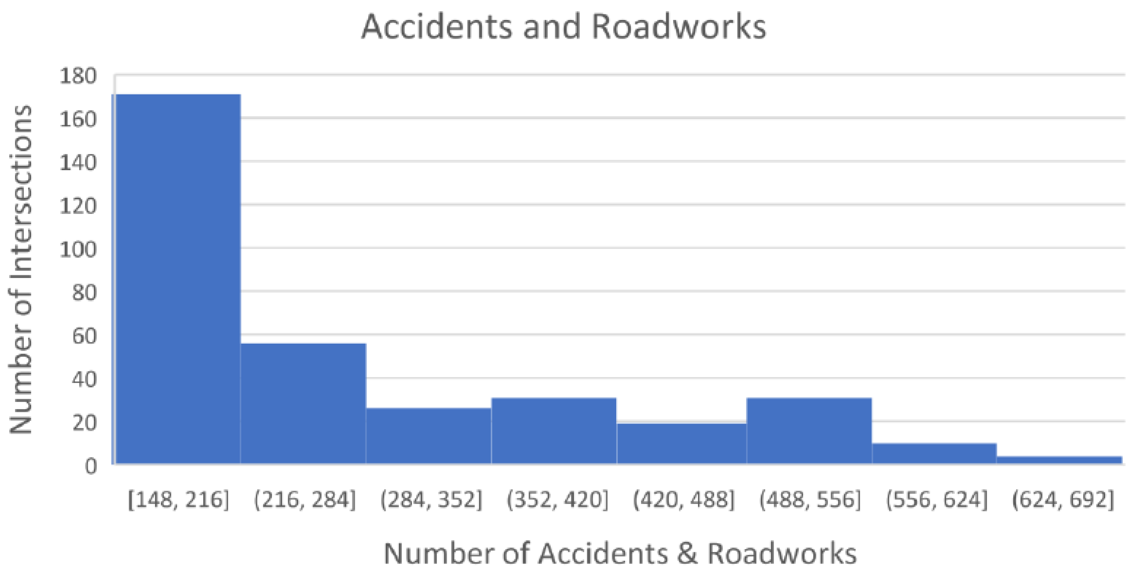
  • Event Distance: As discussed above, traffic patterns change if a nonrecurring event, such as an accident or roadwork, occurs. One of the key contributions of this study is introducing this feature into the process of traffic prediction at intersections. The distance was calculated using the Haversine distance function in Python to find the distance between two coordinates. The value of this feature was 0 if there was no event within 500 m, 1 if the distance was 0–199 m, 2 if the distance was 200–299 m and 3 if the distance was 400–500 m. Figure 2 shows the number of events within 500 m in a subset of intersections in our data set.
  • Time: Clock time was used as a feature after converting it into float:
    t = ( H o u r s + M i n u t e s / 60 )
  • Day/night: This feature distinguishes whether the time is day time or night time.

4. Proposed Methods

4.1. Batch Learning

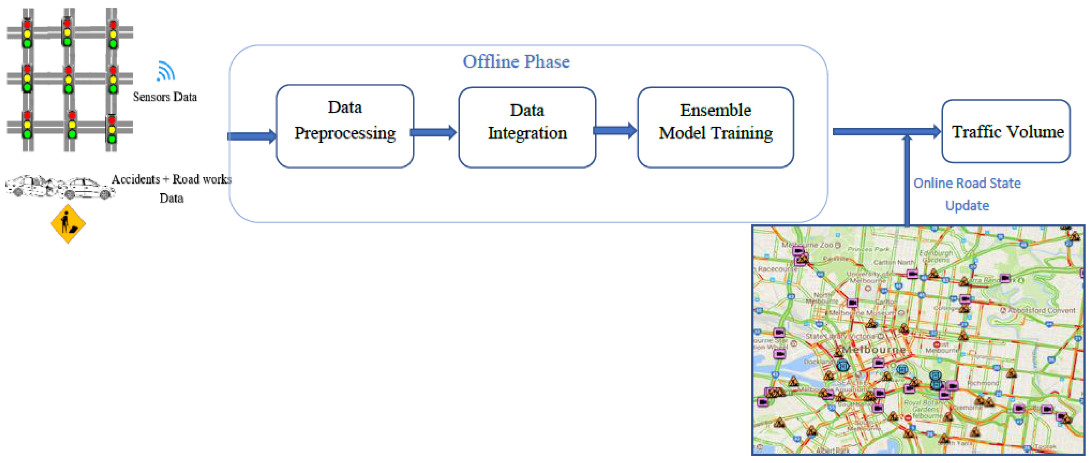
In this section, we introduce the batch-based prediction methods that were used in this study for traffic flow prediction. We propose a two-phase prediction method, as shown in Figure 3. The first phase is the offline phase; in this phase, ensemble decision tree models for prediction are proposed. Ensemble decision tree models were built with different voting methods to select the most popular target label [15]. Ensemble decision tree models combine weak learners to produce a powerful model using one of two methods: boosting or bagging. The gradient boosting trees, GBRT and XGBoost, are two ensemble trees that use boosting, whereas the Random Forest (RF) is an example of an ensemble tree method that uses bagging.
The second phase is the online phase; in this phase, real time information feeds in from the traffic condition website and updates the road’s condition where there is an event, whether it is near the intersection or not. To address the traffic prediction challenges, this method uses nonlinear, nonparametric prediction models in addition to real time updates in the online phase. Moreover, the XGBoost scalable ensemble method for regression is proposed to address the scalability challenge. In the following section, the proposed methods are explained.

4.1.1. Gradient Boosting Regression Trees

The Gradient Boosting Regression Tree model [14] was used in this study to predict the traffic volume at intersections. For a training data set D = { x i , y i } , i = 1 , 2 , , d where d is the number of samples, and each sample consists of m features, an approximation F ( x ) was used to estimate the approximation function by computing the squared error using Equations (2) and (3):
y ¯ = F ( x )
L ( y , y ¯ ) = [ y y ¯ ] 2
For each regression tree, the input space was divided into M regions m 1 , m 2 , , m M , and for each region, a constant value p m was predicted. Thus, the output ( h m ( x ) ) for the input x could be calculated using Equation (4):
h k ( x ) = i = 1 M p i k I ( x m i )
where I = 1 if x m i ; otherwise I = 0 , p i k is the value predicted for the region m i . By applying the training data y i , x i 1 N , GBRT iteratively formed M various single regression trees ( h 1 ( x ) , , h k ( x ) ) . The following equations describe the updating approximation function ( F k ( x ) ) and gradient descent step size ( r k ) :
F k = F k 1 ( x ) + r k i = 1 M p i k I ( x m i )
r k = arg b min j = 1 N L ( y j , F k 1 ( x j ) + b i = 1 M p i k I ( x m i ) )
F k ( x ) = F k 1 ( x ) + i = 1 M y i k I ( x m i ) .
To modify the model to allow it to choose an optimal value ( y i k ) for each of the tree’s regions, m i , p i k was simply ignored. Therefore, Equation (3) was modified as follows:
y i k = arg y min x i m i k L ( y i , F k 1 ( x i ) + y ) = arg y min x i m i k ( y ¯ i y ) 2 .
GBRT uses the stage-wise approach to build the model. At each alteration, the model is updated by minimising the loss function value. In addition, GBRT uses a shrinkage strategy to avoid over-fitting. A learning rate is used for this purpose, where the output of each tree model is scaled by using a value between 0 and 1, as explained in Equations (9) and (10):
F k ( x ) = F k 1 ( x ) + v h k w h e r e v [ 0 , 1 ]
y ¯ i = L ( y i , F ( x i ) F ( x i F k ( x ) = F k 1 ( x ) .
The best shrinkage is obtained when the v value is small. It is used to reduce the loss function at each iteration in order to avoid over-fitting. However, using a small learning rate value could increase the number of trees. The maximum level of the tree (i.e., depth of the tree) is another parameter that needed to be determined. It represents the number of splits and the complexity of a tree. By increasing the depth of the tree, the performance of GBRT is enhanced, because the interactions between features increase. Therefore, to ensure optimal performance of the GBRT, the tree complexity and learning rate values have to be chosen carefully based on the evaluation of the results obtained using the test data set.

4.1.2. Random Forest

The second type of ensemble learning method used based on the decision tree was Random Forest (RF). The procedure of this method can be summarised as follows [15]:
  • Input: An n-dimensional vector ( x ).
  • Output: A predictor (y).
  • Step 1: Bootstrap sampling. In this step, the RF selects a random number of data points with replacement to generate a new training set. Unselected examples are marked as out-of-bag (OOB).
  • Step 2: Decision tree generation. A fully grown decision tree is constructed in this step using the training set without pruning. At each node split, the best feature set from a random number of features subsets is selected until there are no more splits.
  • Repetition: Step 1 and step 2 are repeated until C number of trees is reached.
  • Step 3: C output values are aggregated to obtain the final output (y) by taking the mean of the output values of all the generated trees, as described in Equation (11):
    y ( x ) = 1 J j = 1 J h j ( x )
    where x is the set of input samples, and h j ( x ) is the output of the jth tree.

4.2. XGBoost

XGBoost [16] is a scalable learning system that has a recognised impact in solving machine learning challenges in different application domains. The speed of XGBoost is much faster than that of common machine learning methods, and it can efficiently process billions of data in a parallel and distributed way.
Several algorithmic improvements and the ability to handle sparse data are other features of this model. Sparse input is common in many real-world problems due to several reasons, such as missing data and multiple zero values. Therefore, sparsity-aware data is an important feature that should be included in the algorithm. XGBoost provides this feature by visiting non-missing data only. For the missing data, the algorithm adds the default direction to each tree node; if the value is not provided in the sparse matrix, the input is classified into the default direction. The optimal value of the default direction is learnt from the data. This improvement makes the algorithm faster by making the computation time linear to the number of missing data. The second feature for XGBoost is using column block for parallel learning. XGBoost uses a memory unit called block to store data in a compressed column format. Each column is sorted according to the feature values.

4.3. Online Learning

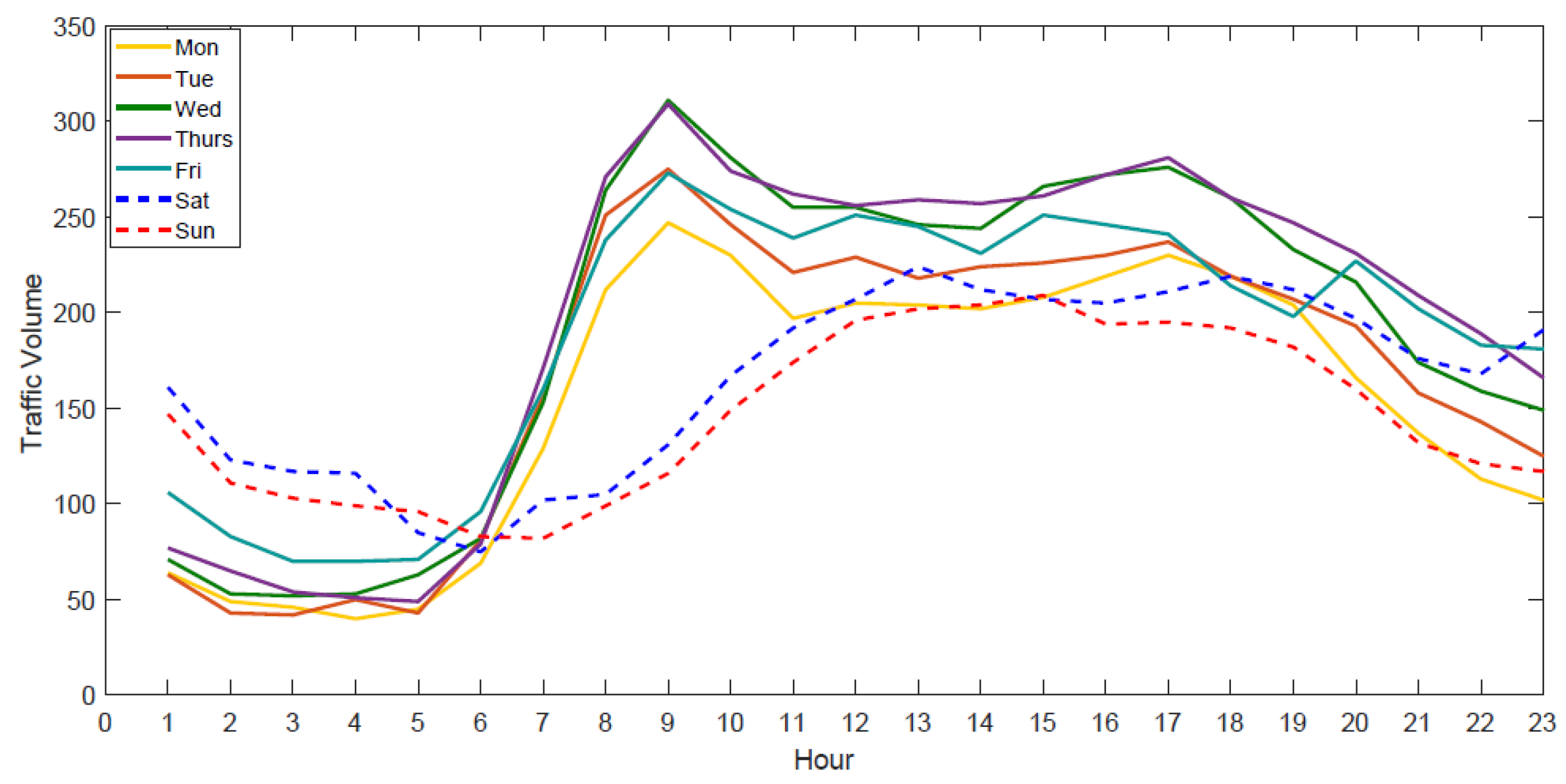
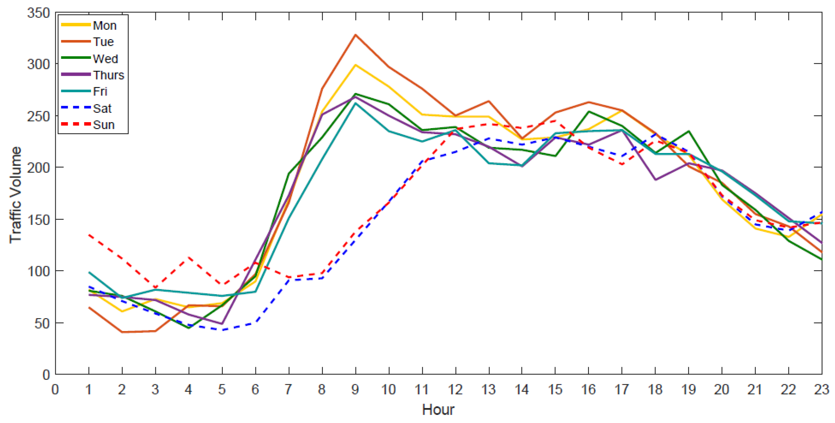
The main disadvantage of batch learning methods is that they require the whole data set to be available in the main memory or the hard disk. The drawbacks appear when the size of the data is large, and also when a long time period is needed to collect the data. In addition, if the data is dynamically changing, then the probability of concept drift occurring will increase. As is clearly shown in Figure 4 and Figure 5, there are variations in traffic patterns when an accident or roadwork appears. To demonstrate this, we first divided the final data set into two parts based on event occurrences. For both parts, we then calculated the average traffic volume per hour for seven days. We found that traffic decreased from normal levels on all days, especially during hours six to thirteen, when the events occurred. In the batch learning scheme, we introduced online updates about events. However, if a new event that was not in the training data set appeared, it caused a prediction error. Therefore, due to this dynamic traffic problem, an incremental learning model was deemed to be useful. With this model, training and learning are done in the same phase, and the model itself is updated for each new example. In this paper, a Fast Incremental Model Tree with Drift Detection (FIMT-DD) is proposed for online traffic prediction using multiple sources of data from sensors installed in intersections as well as accident and roadwork data.
Initially, the algorithm begins with an empty leaf. It then reads the examples coming in sequence based on the arrival time. Following this, the attributes are divided based on the split criterion explained in the next section. If a change is detected, then the model will update and adapt to the change. The following sections present the related details [17].
Split Criterion: There are several techniques that may be used to implement the split criterion To find the best attributes in the samples, the Hoeffding bound is used. In FIMT-DD, incremental standard deviation reduction (SDR) is employed. For example, if the data set is S with size M, the data will be split into two subsets by k A of attribute A. These two sets will be S L and S R , and they will have sizes M L and M R , respectively.
The following formulas were used:
S D R = ( k A ) = s d ( S ) M L M s d ( S L ) M R M s d ( S R )
s d ( S ) = 1 M ( i = 1 M ( y i y ) 2 ) = 1 M ( i = 1 M ( y i 2 1 M ( i = 1 M y i ) 2 ) .
From Equations (15) and (16), it can be observed that the number of instances of passing leaf nodes and the values of y and y 2 , which are the predicted attributes, are maintained by this algorithm. Moreover, R is a real-value random variable within the range of 0 and 1. Given that L A and L B represent the best possible splits of attributes A and B, respectively, real numbers r 1 , r 2 , , r n can be used to represent the r value for each stream. The high confidence interval of the mean random variables can be found by the Hoeffding bound probability, which can be used to find 1 – δ , the average of the random sample of N variables with range R and distance ε . The following formula can be used to calculate ε :
ε = R 2 l n ( 1 δ ) 2 M .
Numerical attributes: The FIMT-DD algorithm employs the Extended Binary Search Tree (E-BST) model. This assists in the online sorting sequence process. E-BST achieves this by incorporating two arrays of three elements. One of the arrays is used to reserve the statistics to differentiate the values, thereby determining whether they are less than or equal to the key. In addition, it determines various aspects, with the structures incrementally updated at a new leaf.
Linear models in leaves: The weights in the FIMT-DD algorithm are updated at every instance in the streams. These weights are enclosed by the parameters, which are from the perceptron and are given in the form of a linear equation.

5. Results

5.1. Features Importance

First, we evaluated the importance of our features for each prediction model. From Table 2, we can see event distance represented 24% of the total features for the GBRT and 22.37% for the XGBoost model. However, it was only 16.36% for RF as RF selects the features randomly; therefore, the value is lower. In addition, the time feature was 38.36% for GBRT and 15.1% for RF and 46.9% for XGBoost, respectively. Moreover, the day of the week feature was 24.4% for GBRT, 2.63% for RF, and 26.78% for XGBoost. Another feature was whether the day was a weekend or a weekday; the importance levels of this feature were 40.3% and 4.2%, 0.1% for GBRT, RF and XGBoost, respectively. The next feature was the time of the day (whether it was night or day time) with the results showing 9% for GBRT, 61.7% for RF, and 1.76% for XGBoost. Finally, the least important feature for all models was whether the time was during peak hours or not, with the results being 1.07%, 0.001%, and 2.17% for GBRT, RF, and XGBoost, respectively. Each method has a different way to choose the data points for training, for example, RF selects the data points randomly. We conclude that adding the event distance feature can increase the accuracy of traffic volume prediction when an event such as an accident or roadwork occurs near an intersection.

5.2. Model Comparison

In the following section, we compare the accuracy of the proposed methods in two parts: first, using batch learning methods and second, using online learning methods. The prediction models used for batch learning were those provided in the Scikit-learn machine learning package [52] and the XGBoost package [53]. Regarding the FIMT-DD model for online leaning, we used the Moa package [54]. All the experiments were conducted using a computer with Intel Core i7 and 8 GB RAM.
For the evaluation, ten-fold cross-validation was used. We used two metrics for the performance evaluation, the Mean Squared Error (MSE) and the Mean Absolute Error (MAE). The metrics were calculated using the following equations, where Y ¯ is the estimated output and Y is the ground truth:
M S E = 1 n t = 1 n ( Y t Y ¯ t ) 2
M A E = 1 n t = 1 n Y t Y ¯ t .

5.3. Results of Batch Learning Methods

We compared the accuracy of the XGBoost, GBRT, RF, RT and SVR methods using the MSE and MAE. Two types of comparisons were made: First, we compared the error rates for the prediction methods; second, we compared the error rates for all methods when using features from sensors only and when we used accident and roadwork data with the sensor data. From Figure 6a, we identified two types of results: First, we compared the error values of the different methods and examined whether the new feature improved the prediction accuracy. To set the parameters of the models, several values were examined. The best accuracy was obtained when we set the following parameters: For all decision tree models, the tree depth was 4, and for the GBRT, the number of estimators was 100 and the learning rate was 0.1.
We found that the MSEs for the SVR, RT, GBRT, RF, and XGBoost approaches were equal to 0.6474, 06807, 0.6721, 0.6874 and 0.6721, respectively, when only the sensor data were used. However, the accuracy was improved by different degrees when the event data were integrated with the sensor data, where the MSEs for the SVR, RT, GBRT, RF, and XGBoost methods were equal to 0.6272, 0.6754, 0.6535, 0.6776 and 0.6534 respectively. In summary, the best MSE was reported for SVR when the event data were added, followed by the XGBoost and GBRT.
The next metric was the MAE, as shown in Figure 6b, where the prediction model errors were 1.4420, 14383, 1.4281, 1.4405 and 1.4300 for the SVR, RT, GBRT, RF, and XGBoost methods, respectively. These values became 1.3637, 1.3446, 1.3095, 1.3605 and 1.3094, respectively, when the events data was included. We concluded that XGBoost has the best accuracy, followed by GBRT.
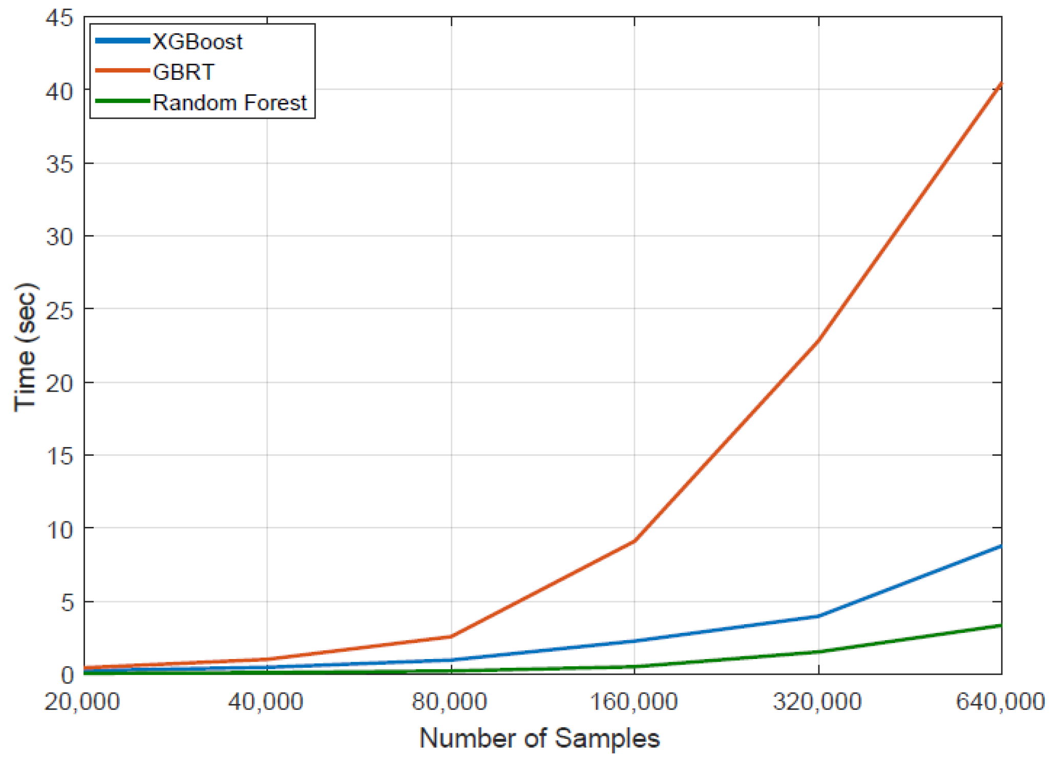
Finally, we evaluated and compared the accuracy of the proposed methods using different sized data. The traffic data were generated continuously, so they had a high volume. Therefore, this experiment needed to examine the efficiency levels of the methods when the number of samples was incremently increased. Figure 7 shows that the proposed methods recorded varying time complexities when the size of the input data increased. In the evaluation, we used a number of samples (n) from 20,000 to 640,000 to investigate which method had a consistent time rate when the volume of data was increased. Three methods required less than 1 second, with a slight difference between them when the volume of data was equal to 20,000. However, when the volume of the data was increased to 80,000, the difference was noticeable, as the time needed for the GBRT increased, reaching nearly 40 s when the data size increased to 460,000. However, the time required by XGBoost increased when the number of samples was greater than 32,000, In summary, the results illustrate that RF requires less time than XGBoost when the number of samples is large. However, XGBoost has better accuracy and good time complexity. On the other hand, GBRT requires more time if the data set is large.

5.4. Results of Online Learning Methods

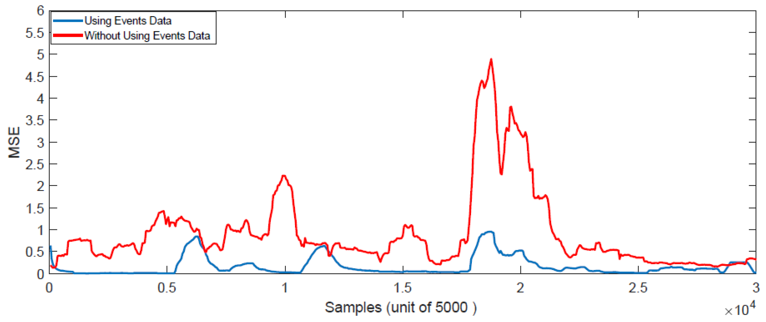
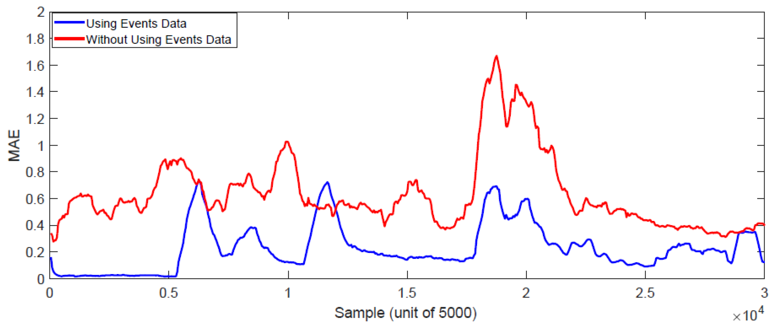
This section presents the evaluation using the online learning method FIMT-DD for traffic flow prediction. In addition, this section conducts a comparison between the batch learning methods discussed in Method 1, Section 2.5, and the FIMT-DD method using two metrics: the Mean Absolute Error (MAE) and the Mean Squared Error (MSE). First, Figure 8 shows the values of MSE during the learning and prediction process, where each unit in the graph represents 5000 examples as the size of the window. The figure clearly shows the importance of using event data to decrease the prediction error. We can also see that the error starts high and then decreases. When the new, unseen examples appear, the error begins to increase. After updating the model, it decreases again. This is due to its ability to process the concept drift and update the model incrementally. The same scenario is apparent in Figure 9, which shows the results of MAE.
Second, Figure 10a illustrates the comparison between the ensemble models, GBRT, RF, and XGBoost, and the FIMT-DD method. It is clearly shown that the FIMT-DD method is less prone to error than the other methods, as it reports that the MSE is 0.774 without using event data, and it is significantly reduced to 0.1089 after including the event data. Moreover, another comparison to MAE is shown in Figure 10b, where the value of the error is 0.63 without using event data, and it reduces to 0.23 after using event data. The results indicate that the FIMT-DD method outperforms the GBRT, RF, and XGBoost learning methods. In addition, it requires only 1.135 s of training and testing to process one year of data.
We conclude that the online learning method should be recommended for traffic flow prediction due to the dynamic changes in traffic patterns when events are occurring. In addition, as the method uses a type of data stream processing that is done online, there is no need to store the whole data set in active memory, which helps to solve the scalability issue.

6. Conclusions

Accurate traffic prediction is important for intelligent transportation systems and smart cities. In this paper, the particular problem of traffic prediction at intersections in city centers is investigated. Based on the fact that accidents and roadworks will affect traffic patterns significantly at intersections, a novel approach for intersection traffic prediction was proposed which involves incorporating multiple sources of data for model training. In particular, this uses accident and roadwork data in addition to traffic volume data. Three ensemble decision tree algorithms (i.e., GBRT, RF, and XGBoost) were adopted to train the prediction model in a batch learning style. In addition, an online learning scheme was proposed, in which the FIMT-DD algorithm is adopted to update the model in real time. Real-world data sets collected from Melbourne, Victoria, Australia were used in the evaluation, and the results show the effectiveness of the proposed methods in reducing the prediction error, especially for the online learning scheme. In future work, we plan to explore an ensemble model of FIMT-DD as well as the distributed traffic data processing framework for vehicular networks.

Author Contributions

Conceptualization, W.A. and S.W.; Methodology, W.A., W.Z. and S.W.; Validation, W.Z. and S.W. and Y.W.; Writing—Original Draft Preparation, W.A. and S.W.; Writing—Review & Editing, W.Z. and Y.W.; Visualization, W.A. and Y.W.; Supervision, S.W. and Y.W.; Funding Acquisition, Y.W.

Funding

This research was funded by NSFC (Grant number 61802080).

Conflicts of Interest

The authors declare no conflict of interest.

References

  1. Mitrovic, N.; Asif, M.T.; Dauwels, J.; Jaillet, P. Low-dimensional models for compressed sensing and prediction of large-scale traffic data. IEEE Trans. Intell. Transp. Syst. 2015, 16, 2949–2954. [Google Scholar] [CrossRef]
  2. Cai, J.; Wang, Y.; Liu, Y.; Luo, J.Z.; Wei, W.; Xu, X. Enhancing network capacity by weakening community structure in scale-free network. Future Gener. Comput. Syst. 2017, 87, 765–771. [Google Scholar] [CrossRef]
  3. Peng, S.; Wang, G.; Xie, D. Social influence analysis in social networking Big Data: Opportunities and challenges. IEEE Netw. 2017, 31, 11–17. [Google Scholar] [CrossRef]
  4. Peng, S.; Yang, A.; Cao, L.; Yu, S.; Xie, D. Social influence modeling using information theory in mobile social networks. Inf. Sci. 2017, 379, 146–159. [Google Scholar] [CrossRef]
  5. Chen, S.; Wang, G.; Yan, G.; Xie, D. Multi-dimensional fuzzy trust evaluation for mobile social networks based on dynamic community structures. Concurr. Comput.-Pract. Exp. 2017, 29, e3901. [Google Scholar] [CrossRef]
  6. Zheng, J.; Bhuiyan, M.Z.A.; Liang, S.; Xing, X.; Wang, G. Auction-based adaptive sensor activation algorithm for target tracking in wireless sensor networks. Future Gener. Comput. Syst. 2014, 39, 88–99. [Google Scholar] [CrossRef]
  7. Xing, X.; Guojun, W.; Jie, L. Collaborative Target Tracking in Wireless Sensor Networks. Ad Hoc Sens. Wirel. Netw. 2014, 23, 117–135. [Google Scholar]
  8. Liu, Q.; Wang, G.; Liu, X.; Peng, T.; Wu, J. Achieving reliable and secure services in cloud computing environments. Comput. Electr. Eng. 2017, 59, 153–164. [Google Scholar] [CrossRef]
  9. Lv, Y.; Duan, Y.; Kang, W.; Li, Z.; Wang, F.Y. Traffic flow prediction with big data: A deep learning approach. IEEE Trans. Intell. Transp. Syst. 2015, 16, 865–873. [Google Scholar] [CrossRef]
  10. Shirazi, M.S.; Morris, B.T. Looking at intersections: A survey of intersection monitoring, behavior and safety analysis of recent studies. IEEE Trans. Intell. Transp. Syst. 2017, 18, 4–24. [Google Scholar] [CrossRef]
  11. National Highway Traffic Safety Administration. Crash Factors in Intersection-Related Crashes: An On-Scene Perspective. 2018. Available online: http://www-nrd.nhtsa.dot.gov/Pubs/811366.pdf (accessed on 15 January 2018).
  12. Anantharam, P.; Thirunarayan, K.; Marupudi, S.; Sheth, A.P.; Banerjee, T. Understanding city traffic dynamics utilizing sensor and textual observations. In Proceedings of the 30th Conference on Artificial Intelligence (AAAI-2016), Phoenix, AZ, USA, 12–17 February 2016; pp. 3793–3799. [Google Scholar]
  13. Polson, N.G.; Sokolov, V.O. Deep learning for short-term traffic flow prediction. Transp. Res. Part C Emerg. Technol. 2017, 79, 1–17. [Google Scholar] [CrossRef] [Green Version]
  14. Zhang, Y.; Haghani, A. A gradient boosting method to improve travel time prediction. Transp. Res. Part C Emerg. Technol. 2015, 58, 308–324. [Google Scholar] [CrossRef]
  15. Ahmad, M.W.; Mourshed, M.; Rezgui, Y. Trees vs. Neurons: Comparison between random forest and ANN for high-resolution prediction of building energy consumption. Energy Build. 2017, 147, 77–89. [Google Scholar] [CrossRef]
  16. Chen, T.; Guestrin, C. Xgboost: A scalable tree boosting system. In Proceedings of the 22th ACM SIGKDD International Conference on Knowledge Discovery and Data Mining, San Francisco, CA, USA, 13–17 August 2016; pp. 785–794. [Google Scholar]
  17. Wibisono, A.; Jatmiko, W.; Wisesa, H.A.; Hardjono, B.; Mursanto, P. Traffic big data prediction and visualization using fast incremental model trees-drift detection (FIMT-DD). Knowl.-Based Syst. 2016, 93, 33–46. [Google Scholar] [CrossRef]
  18. Hamed, M.M.; Al-Masaeid, H.R.; Said, Z.M.B. Short-term prediction of traffic volume in urban arterials. J. Transp. Eng. 1995, 121, 249–254. [Google Scholar] [CrossRef]
  19. Lee, S.; Fambro, D. Application of subset autoregressive integrated moving average model for short-term freeway traffic volume forecasting. Transp. Res. Rec. 1999, 1678, 179–188. [Google Scholar] [CrossRef]
  20. Williams, B.M.; Hoel, L.A. Modeling and forecasting vehicular traffic flow as a seasonal ARIMA process: Theoretical basis and empirical results. J. Transp. Eng. 2003, 129, 664–672. [Google Scholar] [CrossRef]
  21. Min, X.; Hu, J.; Zhang, Z. Urban traffic network modeling and short-term traffic flow forecasting based on GSTARIMA model. In Proceedings of the 13th International IEEE Annual Conference on Intelligent Transportation Systems, Madelra Island, Portugal, 19–22 September 2010; pp. 1535–1540. [Google Scholar]
  22. Asif, M.T.; Dauwels, J.; Goh, C.Y.; Oran, A.; Fathi, E.; Xu, M.; Dhanya, M.M.; Mitrovic, N.; Jaillet, P. Spatiotemporal patterns in large-scale traffic speed prediction. IEEE Trans. Intell. Transp. Syst. 2014, 15, 794–804. [Google Scholar] [CrossRef]
  23. Kim, Y.J.; Hong, J.S.; Oh, S. Urban traffic flow prediction system using a multifactor pattern recognition model. IEEE Trans. Intell. Transp. Syst. 2015, 16, 2744–2755. [Google Scholar]
  24. Zhan, H.; Gomes, G.; Li, X.S.; Madduri, K.; Sim, A.; Wu, K. Consensus Ensemble System for Traffic Flow Prediction. IEEE Trans. Intell. Transp. Syst. 2018, 1–12. [Google Scholar] [CrossRef]
  25. Clark, S. Traffic prediction using multivariate nonparametric regression. J. Transp. Eng. 2003, 129, 161–168. [Google Scholar] [CrossRef]
  26. Zhao, J.; Sun, S. High-order Gaussian process dynamical models for traffic flow prediction. IEEE Trans. Intell. Transp. Syst. 2016, 17, 2014–2019. [Google Scholar] [CrossRef]
  27. Dell’Acqua, P.; Bellotti, F.; Berta, R.; De Gloria, A. Time-aware multivariate nearest neighbor regression methods for traffic flow prediction. IEEE Trans. Intell. Transp. Syst. 2015, 16, 3393–3402. [Google Scholar] [CrossRef]
  28. Chen, D. Research on traffic flow prediction in the big data environment based on the improved RBF neural network. IEEE Trans. Ind. Inf. 2017, 13, 2000–2008. [Google Scholar] [CrossRef]
  29. Xu, Y.; Kong, Q.J.; Klette, R.; Liu, Y. Accurate and interpretable Bayesian MARS for traffic flow prediction. IEEE Trans. Intell. Transp. Syst. 2014, 15, 2457–2469. [Google Scholar] [CrossRef]
  30. Lei, Y.; Qiu, G.; Zheng, L.; Huang, J. Fast Near-Duplicate Image Detection Using Uniform Randomized Trees. ACM Trans. Multimed. Comput. Commun. Appl. 2014, 10. [Google Scholar] [CrossRef]
  31. Chen, Z.; Peng, L.; Gao, C.; Yang, B.; Chen, Y.; Li, J. Flexible neural trees based early stage identification for IP traffic. Soft Comput. 2017, 21, 2035–2046. [Google Scholar] [CrossRef]
  32. Alajali, W.; Zhou, W.; Wen, S. Traffic Flow Prediction for Road Intersections Safety. In Proceedings of the 2nd IEEE International Conference on Smart City Innovations (IEEE SCI 2018), Guangzhou, China, 8–12 October 2018. [Google Scholar]
  33. Castro-Neto, M.; Jeong, Y.S.; Jeong, M.K.; Han, L.D. Online-SVR for short-term traffic flow prediction under typical and atypical traffic conditions. Expert Syst. Appl. 2009, 36, 6164–6173. [Google Scholar] [CrossRef]
  34. Jeong, Y.S.; Byon, Y.J.; Castro-Neto, M.M.; Easa, S.M. Supervised weighting-online learning algorithm for short-term traffic flow prediction. IEEE Trans. Intell. Transp. Syst. 2013, 14, 1700–1707. [Google Scholar] [CrossRef]
  35. Li, J.; Sun, L.; Yan, Q.; Li, Z.; Srisa-an, W.; Ye, H. Significant permission identification for machine learning based android malware detection. IEEE Trans. Ind. Inf. 2018, 14, 3216–3225. [Google Scholar] [CrossRef]
  36. Meng, W.; Jiang, L.; Wang, Y.; Li, J.; Zhang, J.; Xiang, Y. JFCGuard: Detecting juice filming charging attack via processor usage analysis on smartphones. Comput. Secur. 2017, 76, 252–264. [Google Scholar] [CrossRef]
  37. Wu, T.; Wen, S.; Xiang, Y.; Zhou, W. Twitter spam detection: Survey of new approaches and comparative Study. Comput. Secur. 2018, 76, 265–284. [Google Scholar] [CrossRef]
  38. Liu, Y.; Ling, J.; Liu, Z.; Shen, J.; Gao, C. Finger vein secure biometric template generation based on deep learning. Soft Comput. 2018, 22, 2257–2265. [Google Scholar] [CrossRef]
  39. Yuan, C.; Li, X.; Wu, Q.; Li, J.; Sun, X. Fingerprint liveness detection from different fingerprint materials using convolutional neural network and principal component analysis. CMC-Comput. Mater. Contin. 2017, 53, 357–371. [Google Scholar]
  40. Meng, W.; Wang, Y.; Wong, D.S.; Wen, S.; Xiang, Y. TouchWB: Touch behavioral user authentication based on web browsing on smartphones. J. Netw. Comput. Appl. 2018, 117, 1–9. [Google Scholar] [CrossRef]
  41. Jiang, J.; Wen, S.; Yu, S.; Xiang, Y.; Zhou, W. Identifying propagation sources in networks: State-of-the-art and comparative studies. IEEE Commun. Surv. Tutor. 2017, 19, 465–481. [Google Scholar] [CrossRef]
  42. Wen, S.; Haghighi, M.S.; Chen, C.; Xiang, Y.; Zhou, W.; Jia, W. A sword with two edges: Propagation studies on both positive and negative information in online social networks. IEEE Trans. Comput. 2015, 64, 640–653. [Google Scholar] [CrossRef]
  43. Wang, Y.; Wen, S.; Xiang, Y.; Zhou, W. Modeling the propagation of worms in networks: A survey. IEEE Commun. Surv. Tutor. 2014, 16, 942–960. [Google Scholar] [CrossRef]
  44. Li, P.; Li, J.; Huang, Z.; Gao, C.Z.; Chen, W.B.; Chen, K. Privacy-preserving outsourced classification in cloud computing. Clust. Comput. 2017. [Google Scholar] [CrossRef]
  45. Li, P.; Li, J.; Huang, Z.; Li, T.; Gao, C.Z.; Yiu, S.M.; Chen, K. Multi-key privacy-preserving deep learning in cloud computing. Future Gener. Comput. Syst. 2017, 74, 76–85. [Google Scholar] [CrossRef]
  46. Li, J.; Zhang, Y.; Chen, X.; Xiang, Y. Secure attribute-based data sharing for resource-limited users in cloud computing. Comput. Secur. 2018, 72, 1–12. [Google Scholar] [CrossRef]
  47. Gao, C.Z.; Cheng, Q.; Li, X.; Xia, S.B. Cloud-assisted privacy-preserving profile-matching scheme under multiple keys in mobile social network. Clust. Comput. 2018. [Google Scholar] [CrossRef]
  48. Luo, E.; Liu, Q.; Abawajy, J.H.; Wang, G. Privacy-preserving multi-hop profile-matching protocol for proximity mobile social networks. Future Gener. Comput. Syst. 2017, 68, 222–233. [Google Scholar] [CrossRef]
  49. Gao, C.; Cheng, Q.; He, P.; Susilo, W.; Li, J. Privacy-preserving Naive Bayes classifiers secure against the substitution-then-comparison attack. Inf. Sci. 2018, 444, 72–88. [Google Scholar] [CrossRef]
  50. VicTraffic. Available online: https://traffic.vicroads.vic.gov.au/ (accessed on 15 January 2018).
  51. Victorian Government Data Directory. Available online: https://www.data.vic.gov.au/ (accessed on 15 January 2018).
  52. Scikit-learn. Available online: http://scikit-learn.org/stable/ (accessed on 15 January 2018).
  53. XGBoost. Available online: https://github.com/dmlc/xgboost (accessed on 15 January 2018).
  54. Moa: Massive Online Analysis. Available online: https://moa.cms.waikato.ac.nz/ (accessed on 15 January 2018).
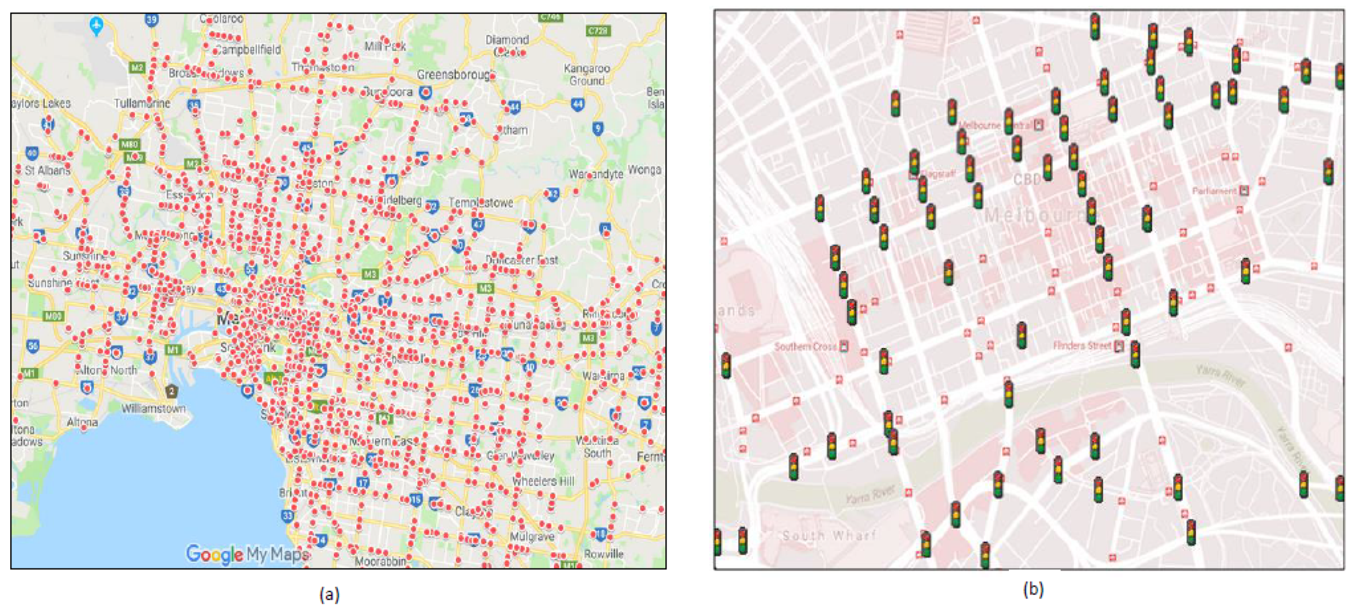
Figure 1. Intersection locations for the traffic volume data set [51]. (a) The 4598 intersections across Melbourne, Victoria, Australia and some suburban areas covered by the original data set. (b) The intersections within the Melbourne Central Business District (CBD) that we focused on in this work.
Symmetry 10 00386 g001
Figure 2. The number of accidents that occurred within 500 m of 350 intersections in 2014.
Symmetry 10 00386 g002
Figure 3. The framework of batch learning.
Symmetry 10 00386 g003
Figure 4. Average traffic volume on days with events at sensor #2906.
Symmetry 10 00386 g004
Figure 5. Average traffic volume on days without events at sensor #2906.
Symmetry 10 00386 g005
Figure 6. Accurate results of batch learning methods. (a) Mean Squared Error (MSE) results. (b) Mean Absolute Error (MAE) results.
Symmetry 10 00386 g006
Figure 7. Time results of the ensemble models with different size of data.
Symmetry 10 00386 g007
Figure 8. MSE results of Fast Incremental Model Trees with Drift Detection (FIMT-DD) online learning.
Symmetry 10 00386 g008
Figure 9. MAE results of FIMT-DD online learning.
Symmetry 10 00386 g009
Figure 10. Comparison of results from the batch learning and online learning methods. (a) MSE results. (b) MAE results.
Symmetry 10 00386 g010
Table 1. Description of data sets.
Data SetDuration# of RecordsType# of SensorsTime Interval
Traffic Volume1 January 2014–31 December 201428,992 per intersectionPublic459815 min
Car Accidents1 January 2014–31 December 201414,247Public--
Roadworks1 January 2014–31 December 20145637Public--
Table 2. Importance of features.
Prediction ModelTimeDayWeekendPeakDay NightEvent Distance
GBRT0.38360.2440.40300.01070.09030.2409
RF0.15100.02630.04220.00010.61720.1633
XGBoost0.46920.26780.0010.02170.01760.2237