The New Similarity Measure and Distance Measure of a Hesitant Fuzzy Linguistic Term Set Based on a Linguistic Scale Function

Abstract

The existing cosine similarity measure for hesitant fuzzy linguistic term sets (HFLTSs) has an impediment as it does not satisfy the axiom of similarity measure. Due to this disadvantage, a new similarity measure combining the existing cosine similarity measure and the Euclidean distance measure of HFLTSs is proposed, which is constructed based on a linguistic scale function; the related properties are also given. According to the relationship between the distance measure and the similarity measure, a corresponding distance measure between HFLTSs is obtained. Furthermore, we generalize the technique for order preference by similarity to an ideal solution (TOPSIS) method to the obtained distance measure of the HFLTSs. The principal advantages of the proposed method are that it cannot only effectively transform linguistic information in different semantic environments, but it can also avoid the shortcomings of existing the cosine similarity measure. Finally, a case study is conducted to illustrate the feasibility and effectiveness of the proposed method, which is compared to the existing methods.

1. Introduction

In many multi-criteria decision making (MCDM) problems, because of the incomplete information and the complexity of the decision-making environment, crisp numbers cannot describe the relevant decision information. Thus Zadeh [1] proposed the fuzzy set (FS) $A=\{\left(x_j,{\mu }_A\left(x_j\right)\right)|x_j\in X\}$ $\left(0\le {\mu }_A\left(x_j\right)\le 1\right)$ on $X=\{x_1,x_2,\cdots ,x_n\},$ where ${\mu }_A\left(x_j\right)$ is the membership degree of $x_j\in X$. Since it was put forward, many scholars have generalized it. For example, Atanassov [2,3] introduced the concepts of the intuitionistic fuzzy set (IFS) and the interval-valued intuitionistic fuzzy set (IVIFS), and Torra [4] proposed the hesitant fuzzy set (HFS). In the past few years, the FS and its extensions have been applied in many fields, such as supplier selection, pattern recognition, and medical diagnosis. As the FS and its extensions mentioned above use crisp numbers to express decision information, they cannot express qualitative evaluation information. For instance, when one expert evaluates the performance of a company, he/she thinks that the performance of the company is very good. Because the evaluation expression is consistent with the human’s cognitive process, it is suitable to express this in a linguistic term set (LTS). To describe the relevant information, Zadeh [5,6,7] proposed the LTS to express the relevant information. A general discrete LTS of seven terms can be represented as $S=\{s_0:verypoor,s_1:poor,s_2:slightlypoor,s_3:fair,s_4:$ $slightlygood,s_5:good,s_6:verygood\}$. Then, the expert’s evaluation about the performance of the company can be represented as $\{s_6\}$. However, due to the uncertainty of the problem in the decision making process, the decision makers cannot express their preferences using only one membership degree of a LTS. In order to express the decision makers’ hesitation about the decision problem, Rodríguez et al. [8] proposed the hesitant fuzzy linguistic term set (HFLTS), which is based on LTS and HFS. The HFLTS makes the representation of the decision information more flexible. Since the HFLTS was proposed, a number of relevant studies and their applications [9,10,11,12,13,14,15,16,17,18,19,20,21,22] have been conducted. For example, Liu et al. [16] presented the fuzzy envelope for HFLTSs and applied it to choose the best alternative. Xu et al. [17] presented the hesitant fuzzy linguistic ordered weighted distance operator, and applied it to plan the selection of enterprise’s large projects. Liao et al. [18] maked a survey on HFLTSs and reviewed the decision making process with hesitant fuzzy linguistic preference (HFLP) relations. Liao et al. [19] proposed the hesitant fuzzy linguistic preference utility set (HFLPUS) and applied the HFLP utility TOPSIS approach to choose the best fire rescue alternative. One thing that they have in common is that they use the subscript of linguistic terms directly in the process of operations, which may cause a loss of information. In order to overcome this problem, the linguistic scale function was introduced by Wang et al. [23], which can assign different numerical values to the linguistic terms set under different circumstances. The linguistic scale function can reflect the preferences of the decision makers in different environments. Since it was put forward, many scholars have studied this subject. For example, Wang et al. [24] presented the Hausdorff distance between the hesitant fuzzy linguistic numbers (HFLNs), based on the linguistic scale function, and developed the TOPSIS and TODIM approaches to it. Liu et al. [25] proposed a distance measure of HFLTSs, which also included the linguistic scale function. Furthermore, Liu et al. [26] proposed the intuitionistic fuzzy linguistic cosine similarity measure and the interval-valued intuitionistic fuzzy linguistic cosine similarity measure, they all contain the linguistic scale function. The research on this field has developed rapidly.

From another perspective, the similarity measure is also an important aspect in MCDM problems, which can measure the similarity degree between two different alternatives. It has been widely studied in the past few years. For example, Song et al. [27] considered the similarity measure between IFSs, and proposed the corresponding distance measure between IF belief functions. Liao et al. [9] presented some similarity measures and distance measures between HFLTSs; Lee et al. [10] proposed a similarity measure based on likelihood relations. For the other studies about the similarity measure, we can refer to [11,12,13]. The cosine similarity measure is also a significant similarity measure; it can be expressed as the inner product of two vectors divided by the product of their lengths [28]. Some scholars have studied the cosine similarity measure [29,30,31]. For instance, Ye [29] introduced a weighted cosine similarity measure between IFSs and they applied it to rank the alternative. Furthermore, Ye [30] presented the cosine similarity measure between interval-valued fuzzy sets (IVFSs) with risk preference, and altered its decision making method depending on decision makers’ preferences. Liao et al. [31] defined the cosine similarity measure between HFLTSs and extended the TOPSIS approach and VIKOR approach to the cosine distance measure. It is already known that the cosine similarity measure proposed by Liao et al. [31] is not a regular similarity measure (because it is not satisfied with the axiom of the similarity measure; the example can be seen in Section 3). If it is applied in MCDM problems, it may cause the decision information to be distorted. Furthermore, the cosine similarity measure defined by Liao et al. [31] used the subscript of linguistic terms directly in process of operations; they did not consider the semantic decision environment, which may cause a loss of information in the decision making process.

Therefore, this paper introduces a new method to construct a similarity measure between HFLTSs; the main motivations and contributions of the paper are given as follows:

(1)

In order to overcome the disadvantage of the similarity measure proposed by Liao et al. [31], a new similarity measure combining the existing cosine similarity measure [31] and the Euclidean distance measure of HFLTSs is proposed in this paper, which can improve the accuracy of the calculation to some extent.

(2)

On the basis of the linguistic scale function, the paper proposes a new similarity measure between two HFLTSs; it is already known that the linguistic scale function can improve the flexibility of the transformation of the linguistic decision information in different semantic environments. The proposed method is capable of expressing the fuzzy linguistic information more flexibly and improving the adaptability of HFLTSs in practice.

(3)

According to the relationship between the similarity measure and the distance measure, this paper proposes a new distance measure of HFLTSs and extends the TOPSIS method to it; it focuses on the differences between different alternatives, which can improve the effectiveness of solving MCDM problems.

The reminder of the paper is given as follows: the background on the MCDM problems, some concepts of LTS and HFLTS, the existing similarity measures of HFLTSs, and the linguistic scale function are reviewed in Section 2. In Section 3, a new score function of HFLTS based on the linguistic scale function, and a new approach to construct the similarity measure of HFLTSs, are presented. The corresponding distance measure is also constructed based on the relationship between the distance measure and the regular similarity measure. In Section 4, we extend the TOPSIS method to the proposed distance measure. In Section 5, a numerical example is given to illustrate the feasibility of the proposed method, and the same numerical example is examined to compare with other methods. Some conclusions and future research are proposed in Section 6.

2. Preliminaries

In this section, we will explain how the MCDM method works, and we review some basic knowledge, including LTS, HFLTS, the score function of HFLTS, and the linguistic scale function. Some existing distance measures and similarity measures of HFLTSs are also introduced. In this paper, we denote $X=\{x_1,x_2,\cdots ,x_n\}$ as the discourse set.

2.1. MCDM

Multi-criteria decision making is an important branch of the decision-making field. There are some common aspects (alternatives and criteria) in MCDM; the typical MCDM problem can be described as follows:

Let $X=\{x_1,x_{72},\cdots ,x_n\}$ be a set of alternatives; let $C=\{c_1,c_2,\cdots ,c_m\}$ be a set of criteria values. The decision matrix $D$ is an $n\times m$ matrix, in which element $d_{ij}$ indicates the performance of the alternative $x_i$ when it is evaluated according to the decision criterion $c_j$ ($i=1,2,\cdots n;j=1,2,\cdots m.$); the decision element $d_{ij}$ is provided by the expert. It is also assumed that the expert has determined the weight of the criteria (denoted as ${\omega }_j,j=1,2,\cdots m$). There are three steps in utilizing the decision-making technique to rank the alternatives [32]: (1) Provide the relevant criteria and alternatives. (2) Collective information calculation. (3) Rank the alternative according to the collective information.

2.2. LTS

LTS is suitable for qualitative description of the decision-making problems, which can be defined as follows:

Definition 1.

Let$S=\{s_i|i=0,1,\cdots ,2t\}$be a finite and totally ordered discrete linguistic term set, where$s_i$is a possible value for a linguistic variable, and$t$is a positive integer [33].

(1) 

The LTS$S$satisfies the following properties:

(2) 

The set$S$is ordered:$s_i\le s_j$if$i\le j$;$max\left(s_i,s_j\right)=s_i$if$s_i\ge s_j$;$min\left(s_i,s_j\right)=s_i$if$s_i\le s_j$;

(3) 

The negation operator is defined:$neg\left(s_i\right)=s_j$. satisfying with$i+j=2t$.

In order to make the description of the given information more accurate, Xu [34] generalized the discrete linguistic term set $S$ to the continuous linguistic term set $\overline{S}$ = $\{s_i|i\in \left[0,\tau \right]\}(\tau >2t)$, where $s_i\le s_j$ if $i\le j$, and $\tau$ is a sufficiently large positive integer.

2.3. HFLTS

The HFLTS permits the membership of an element to be a set of several possible linguistic variable values. In the following, the concept of HFLTS and some related operations of HFLTS are reviewed.

Definition 2.

Given a fixed set$X$, let$S=\{s_i|i=0,1,\cdots ,2t\}$be a LTS, then a HFLTS$H_S$on$X$is expressed by [8]:

$$H_S=\{\left(x_j,h_S\left(x_j,\right)\right)|x_j\in X\}$$

where$h_S\left(x_j\right)$is a subset of linguistic terms in$S$, it represents the membership degrees of the element$x_j$belongs to$X.$For convenience, the element of$h_S\left(x_j\right)$is called the hesitant fuzzy linguistic element (HFLE).

Example 1.

Let$S=\{s_0:verypoor,s_1:poor,s_2:slightlypoor,s_3:fair,s_4:slightlygood,s_5:good,s_6:verygood\}$be a LTS. Two experts evaluate the performance of a company; one thinks the performance of a company is not less than good, the other thinks it is between fair and good. According to Definition 2, the above evaluation information can be represented as$H_S^1=\{s_5,s_6\}$and$H_S^2=\{s_3,s_4,s_5\}$, respectively. The numbers of linguistic terms in$H_S^1$and$H_S^2$are not equal, which is not convenient for computing the similarity measure between$H_S^1$and$H_S^2$.

In order to solve this problem, for any two HFLTSs $H_S^1=\{\left(x_j,h_S^1\left(x_j\right)\right)|x_j\in X\}$ and $H_S^2=\{\left(x_j,h_S^2\left(x_j\right)\right)|x_j\in X\}\left(j=1,2,\cdots ,n\right)$, where $h_S^k\left(x_j\right)=\{s_{{\delta }_l^k}\left(x_j\right)|s_{{\delta }_l^k}\left(x_j\right)\in S,l^k=1,2,\cdots ,L_j^k\}$, if the numbers of $h_S^k\left(x_j\right)$ are not equal, we can let $L_j=max\{L_j^1,L_j^2\}$. Zhu et al. [35] proposed the rules of regulation: for the optimists, they extend the set with fewer numbers of elements by adding the maximum value $s_{{\delta }_l^k}^{+}\left(x_j\right)=\begin{array}{c}max\\ l=L_j^{1}orl=L_j^2\end{array}\{s_{{\delta }_l^k}\left(x_j\right)\}$ until the two sets have the same number of elements; while for the pessimists, they add the minimum value $s_{{\delta }_l^k}^{-}\left(x_j\right)=\begin{array}{c}min\\ l=L_j^{1}orl=L_j^2\end{array}\{s_{{\delta }_l^k}\left(x_j\right)\}$ to the set with fewer numbers of elements. In this paper, we assume that the largest element is added to the set with fewer elements until they have the same number.

The existing score function of HFLTSs is defined as follows:

Definition 3.

Let$S=\{s_i|i=0,1,\cdots ,2t\}$be a LTS;$H_S=\{s_{{\delta }_l^k}\left(x_j\right)|s_{{\delta }_l^k}\left(x_j\right)\in S\}\left(l=1,2,\cdots ,L_j,j=1,2,\cdots ,n\right)$be a HFLTS on$X$, then the score function of$H_S$is [36]:

$$F(H_S)=\frac{1}{n}{\displaystyle {\displaystyle \sum }_{j=1}^n}\overline{\delta }(x_j)-\frac{{{\displaystyle \sum }}_{j=1}^n\left(\frac{1}{L_j}{{\displaystyle \sum }}_{l=1}^{L_j}{\left({\delta }_l\left(x_j\right)-\overline{\delta }\left(x_j\right)\right)}^2\right)}{Var\left(2t\right)}$$

where$\overline{\delta }=\frac{1}{L_j}{\displaystyle {{\displaystyle \sum }}_{l=1}^{L_j}}{\delta }_l\left(x_j\right)$,$Var\left(2t\right)=\frac{{{\displaystyle \sum }}_{i=0}^{2t}{\left(i-t\right)}^2}{2t+1}$.

Lemma 1.

For two HFLTSs$H_S^1$and$H_S^2$, the comparison rules between them are defined as follows [36]:

(1) 

$H_S^1>H_S^2$if and only if$F\left(H_S^1\right)>F\left(H_S^2\right)$;

(2) 

$H_S^1=H_S^2$if and only if$F\left(H_S^1\right)=F\left(H_S^2\right)$.

2.4. Existing Distance and Similarity Measures Between HFLTSs

The Distance and similarity measure are effective tools for describing the deviation and closeness between different alternatives in MCDM problems; the definitions about the existing distance and similarity measures between HFLTSs are given as follows:

Definition 4.

Given a fixed set$X$, suppose that$S=\{s_i|i=0,1,\cdots ,2t\}$be a LTS,$h_S^k\left(x_j\right)=\{s_{{\delta }_l^k}\left(x_j\right)|s_{{\delta }_l^k}\left(x_j\right)\in S,l=1,2,\cdots ,L_j\}$, where$L_j=max\{l\left(h_S^1\left(x_j\right),l(h_S^2\left(x_j\right)\right))$,$l\left(h_S^k\left(x_j\right)\right)$represents the number of elements in$h_S^k\left(x_j\right)$$\left(k=1,2\right)$. For any two HFLTSs$H_S^1=\{\left(x_j,h_S^1\left(x_j\right)\right)|x_j\in X\}$and$H_S^2=\{\left(x_j,h_S^2\left(x_j\right)\right)|x_j\in X\}\left(j=1,2,\cdots ,n\right)$, assume the weight of different element$x_j$is${\omega }_j$$\left(j=1,2,\cdots ,n\right)$, then the weighted Euclidean distance measure between$H_S^1$and$H_S^2$can be defined as follows [9]:

$$D_{\omega HFL}\left(H_S^1,H_S^2\right)={\left({\displaystyle {\displaystyle \sum }_{j=1}^n}\frac{{\omega }_j}{L_j}{\displaystyle {\displaystyle \sum }_{l=1}^{L_j}}{\left(\frac{\left|{\delta }_l^1\left(x_j\right)-{\delta }_l^2\left(x_j\right)\right|}{2t+1}\right)}^2\right)}^{\frac{1}{2}}.$$

(1)

Remark 1.

For all$j=1,2,\cdots ,n$, if the weight${\omega }_j=\frac{1}{n}$, then the weighted Euclidean distance measure$D_{\omega HFL}\left(H_S^1,H_S^2\right)$is reduced to the Euclidean distance measure$D_{HFL}\left(H_S^1,H_S^2\right)$:

$$D_{HFL}\left(H_S^1,H_S^2\right)={\left(\frac{1}{n}\left({\displaystyle {\displaystyle \sum }_{j=1}^n}\frac{1}{L_j}{\displaystyle {\displaystyle \sum }_{l=1}^{L_j}}{\left(\frac{\left|{\delta }_l^1\left(x_j\right)-{\delta }_l^2\left(x_j\right)\right|}{2t+1}\right)}^2\right)\right)}^{\frac{1}{2}}$$

Liao et al. [31] defined a cosine similarity measure between HFLTSs as follows:

Definition 5.

Given a fixed set$X$, suppose that$S=\{s_i|i=0,1,\cdots ,2t\}$is a LTS,$h_S^k\left(x_j\right)=\{s_{{\delta }_l^k}\left(x_j\right)|s_{{\delta }_l^k}\left(x_j\right)\in S,l=1,2,\cdots ,L_j\}$, where$L_j=max\{l\left(h_S^1\left(x_j\right),l(h_S^2\left(x_j\right)\right)\}$,$l\left(h_S^k\left(x_j\right)\right)$represents the number of elements in$h_S^k\left(x_j\right)$$\left(k=1,2\right)$. For any two HFLTSs$H_S^1=\{\left(x_j,h_S^1\left(x_j\right)\right)|x_j\in X\}$and$H_S^2=\{\left(x_j,h_S^2\left(x_j\right)\right)|x_j\in X\}\left(j=1,2,\cdots ,n\right)$, if the weight of different element$x_j$is${\omega }_j$$\left(j=1,2,\cdots ,n\right)$, then the weighted cosine similarity measure can be defined as [31]:

$$Co{s}_{\omega HFL.}\left(H_S^1,H_S^2\right)=\frac{{{\displaystyle \sum }}_{j=1}^n\left(\frac{{\omega }_j}{L_j}{{\displaystyle \sum }}_{l=1}^{L_j}\left(\frac{{\delta }_l^1\left(x_j\right)}{2t+1}·\frac{{\delta }_l^2\left(x_j\right)}{2t+1}\right)\right)}{{\left({{\displaystyle \sum }}_{j=1}^n\left(\frac{{\omega }_j}{L_j}{{\displaystyle \sum }}_{l=1}^{L_j}{\left(\frac{{\delta }_l^1\left(x_j\right)}{2t+1}\right)}^2\right)·{{\displaystyle \sum }}_{j=1}^n\left(\frac{{\omega }_j}{L_j}{{\displaystyle \sum }}_{l=1}^{L_j}{\left(\frac{{\delta }_l^2\left(x_j\right)}{2t+1}\right)}^2\right)\right)}^{\frac{1}{2}}}$$

(2)

Remark 2.

For all$j=1,2,\cdots ,n$, if the weight${\omega }_j=\frac{1}{n}$, then the weighted cosine similarity measure$Co{s}_{\omega HFL}\left(H_S^1,H_S^2\right)$is reduced to the cosine similarity measure$Co{s}_{HFL}(H_{S^{\prime }}^1,H_{S^{\prime }}^2)$:

$$Co{s}_{HFL.}\left(H_S^1,H_S^2\right)=\frac{{{\displaystyle \sum }}_{j=1}^n\left(\frac{1}{L_j}{{\displaystyle \sum }}_{l=1}^{L_j}\left(\frac{{\delta }_l^1\left(x_j\right)}{2t+1}·\frac{{\delta }_l^2\left(x_j\right)}{2t+1}\right)\right)}{{\left({{\displaystyle \sum }}_{j=1}^n\left(\frac{1}{L_j}{{\displaystyle \sum }}_{l=1}^{L_j}{\left(\frac{{\delta }_l^1\left(x_j\right)}{2t+1}\right)}^2\right)·{{\displaystyle \sum }}_{j=1}^n\left(\frac{1}{L_j}{{\displaystyle \sum }}_{l=1}^{L_j}{\left(\frac{{\delta }_l^2\left(x_j\right)}{2t+1}\right)}^2\right)\right)}^{\frac{1}{2}}}$$

(3)

2.5. Linguistic Scale Function

In different semantic decision-making environments, linguistic terms have some differences in expressing alternatives. Bao et al. [37] thought that the information may be distorted when using the subscript of the linguistic term set directly in the process of operations. To solve this problem, Wang et al. [23] put forward the linguistic scale function to calculate the linguistic information. According to the decision-making environment, the decision makers choose a different linguistic scale function, which can express the linguistic information more flexibly in different semantic situations.

Definition 6.

Let$S=\{s_i|i=0,1,\cdots ,2t\}$be a LTS; if${\theta }_i\in R^{+}\left(R^{+}=\{r|r\ge 0,r\in R\}\right)$is a real value, then the linguistic scale function$f$can be defined as follows [22]:

$$f:s_i\to {\theta }_i\left(i=0,1,\cdots ,2t,\right)$$

where$0\le {\theta }_0\le {\theta }_1\le \cdots \le {\theta }_{2t}\le 1$. The linguistic scale function$f$is a strictly monotonically increasing function on the subscript of$s_i$. Actually, the function value${\theta }_i$represents the semantics of the linguistic terms.

Next we introduce three common linguistic scale functions as follows:

$$\left(1\right).f_1\left(s_i\right)={\theta }_i=\frac{i}{2t}{\left(i=0,1,\cdots ,2t\right)}_1).$$

$$\left(2\right).f_2\left(s_i\right)={\theta }_i=\{\begin{array}{cc}\frac{a^t-a^{t-i}}{2a^t-2},\hfill & \hfill \left(i=0,1,\cdots ,t\right);\\ \frac{a^t+a^{i-t}-2}{2a^t-2},\hfill & \hfill \left(i=t+1,t+2,\cdots ,2t\right).\end{array}$$

If the LTS is a set of seven terms, then $a\in \left[1.36,1.4\right]$ [38]. In this paper, we assume that $a=1.4$.

$$\left(3\right).f_3\left(s_i\right)={\theta }_i=\{\begin{array}{cc}\frac{t^{\alpha }-{\left(t-i\right)}^{\alpha }}{2t^{\alpha }},\hfill & \hfill \left(i=0,1,\cdots ,t\right);\\ \frac{t^{\beta }-{\left(t-i\right)}^{\beta }}{2t^{\beta }},\hfill & \hfill \left(i=t+1,t+2,\cdots ,2t\right),\end{array}$$

where $\alpha ,\beta \in \left(0,1\right]$. If the LTS is a set of seven terms, then $\alpha =\beta =0.8$ [39].

Example 2.

Assume that$S=\{s_i|i=0,1,\cdots ,2t\}$be a LTS. When$t=3$, the corresponding linguistic scale functions are$f_1\left(s_i\right)$,$f_2\left(s_i\right)\left(a=1.4\right)$,$f_3\left(s_i\right)\left(\alpha =\beta =0.8\right)$respectively, and the characteristics of the three functions are shown in Figure 1.

Remark 3.

The linguistic scale function$f_1\left(s_i\right)$can be explained as the decision maker’s neutral attitude towards risk; the linguistic scale function$f_2\left(s_i\right)$indicates that the decision maker’s attitude towards risk is changing from aversion to appetite; the linguistic scale function$f_3\left(s_i\right)$indicates that the decision maker’s attitude towards risk is changing from appetite to aversion.

3. The Score Function, Similarity Measure, and Distance Measure Between HFLTSs Based on a Linguistic Scale Function

In this section, we first propose the definition of a new score function of HFLTSs based on a linguistic scale function, then the new similarity measure and its properties are given. Furthermore, we construct a corresponding distance measure based on the relationship between the similarity measure and the distance measure.

3.1. The Score Function Between HFLTSs Based on the Linguistic Scale Function

Definition 7.

Let$S=\{s_i|i=0,1,\cdots ,2t\}$be a LTS,$H_S=\{s_{{\delta }_l^k}\left(x_j\right)|s_{{\delta }_l^k}\left(x_j\right)\in S\}$$\left(l=1,2,\cdots ,L_j,j=1,2,\cdots ,n\right)$be the HFLTS on$X$, and$f$be a linguistic scale function, then the score function of$H_S$is defined as:

$$F^{\ast }(H_S)=\frac{1}{n}{\displaystyle {{\displaystyle \sum }}_{j=1}^n}\overline{f}\left(s_{{\delta }_l}\left(x_j\right)\right)-\frac{{{\displaystyle \sum }}_{j=1}^n\left(\frac{1}{L_j}{{\displaystyle \sum }}_{l=1}^{L_j}{\left(f\left(s_{{\delta }_l}\left(x_j\right)\right)-\overline{f}{s}_{{\delta }_l}\left(x_j\right)\right)}^2\right)}{Va{r}^{\ast }\left(2t\right)},$$

where$\overline{f}\left(s_{{\delta }_l}\left(x_j\right)\right)=\frac{1}{L_j}{\displaystyle {{\displaystyle \sum }}_{l=1}^{L_j}}f\left(s_{{\delta }_l}\left(x_j\right)\right)$,$Va{r}^{\ast }\left(2t\right)={\displaystyle {{\displaystyle \sum }}_{i=0}^{2t}}{\left(f\left(s_i\right)-f\left(s_t\right)\right)}^2$.

Theorem 1.

For any two HFLTSs$H_S^1$and$H_S^2$, the comparison rules between them are defined as follows:

(1) 

If$F^{\ast }\left(H_S^1\right)>F^{\ast }\left(H_S^2\right)$, then$H_S^1>H_S^2$;

(2) 

If$F^{\ast }\left(H_S^1\right)=F^{\ast }\left(H_S^2\right)$, then$H_S^1=H_S^2$.

Example 3.

Let$S=\{s_0:verypoor,s_1:poor,s_2:slightlypoor,s_3:fair,s_4:slightlygood,s_5:good,s_6:$$verygood\}$be a LTS, three HFLTSs are given as follows:$H_S^1=\{s_0,s_1,s_2\}$,$H_S^2=\{s_2,s_3,s_4\}$and$H_S^3=\{s_0,s_2\}$. By Definition 7, if the linguistic scale function$f=f_1\left(s_i\right)=\frac{i}{2t}\left(t=3\right)$, we obtain$F^{\ast }\left(H_S^1\right)=0.1429,F^{\ast }\left(H_S^2\right)=0.4048,F^{\ast }\left(H_S^3\right)=0.1310$, then the ranking of the HFLTSs is$H_S^2>H_S^1$$>H_S^3$. By Definition 3, we can obtain$F\left(H_S^1\right)=0.8323,F\left(H_S^2\right)=2.8333,F\left(H_S^3\right)=0.75$, according to Lemma 1, and it is clearly seen that$H_S^2>H_S^1>H_S^3$, which is same as the proposed score function in Theorem 1.

3.2. The Similarity Measure Between HFLTSs Based on the Linguistic Scale Function

It is already known the regular similarity measure satisfies the following Lemma 2:

Lemma 2.

Let$S=\{s_i|i=0,1,\cdots ,2t\}$be a LTS,$H_S^1$and$H_S^2$be any two HFLTSs; if the similarity measure$S\left(H_S^1,H_S^2\right)$satisfies the following properties [9]:

(1) 

$0\le S\left(H_S^1,H_S^2\right)\le 1$,

(2) 

$S\left(H_S^1,H_S^2\right)=1$if and only if$H_S^1=H_S^2$,

(3) 

$S\left(H_S^1,H_S^2\right)=S\left(H_S^2,H_S^1\right)$.

then the similarity measure$S\left(H_S^1,H_S^2\right)$is a regular similarity measure, and the corresponding distance measure$D\left(H_S^1,H_S^2\right)=1-S\left(H_S^1,H_S^2\right)$.

The cosine similarity measure proposed by Liao et al. [31] is sometimes different from human intuition in practical decision-making problems, and we can determine this from the following Example 4.

Example 4.

When two experts evaluate the performance of a company, they provide their opinions with hesitant fuzzy linguistic information; for the given LTS,$=\{s_0:verypoor,s_1:poor,s_2:slightlypoor,s_3:fair,s_4:slightly$$good,s_5:good,s_6:verygood\}$, and two experts’ evaluations are represented as HFLTSs$H_S^1=\{s_1,s_2\}$and$H_S^2=\{s_2,s_4\}$, respectively.

It is already known $H_S^1\ne H_S^2$, but from using Formula (3) to calculate the similarity measure between $H_S^1$ and $H_S^2$, we have $Co{s}_{HFL}\left(H_S^1,H_S^2\right)=1$. That is to say, the property (2) in Lemma 2 is not satisfied. So, the similarity measure $Co{s}_{HFL}$ proposed by Liao et al. [31] is not a regular similarity measure. On the other hand, the similarity measure $Co{s}_{HFL}$ as defined by Liao et al. 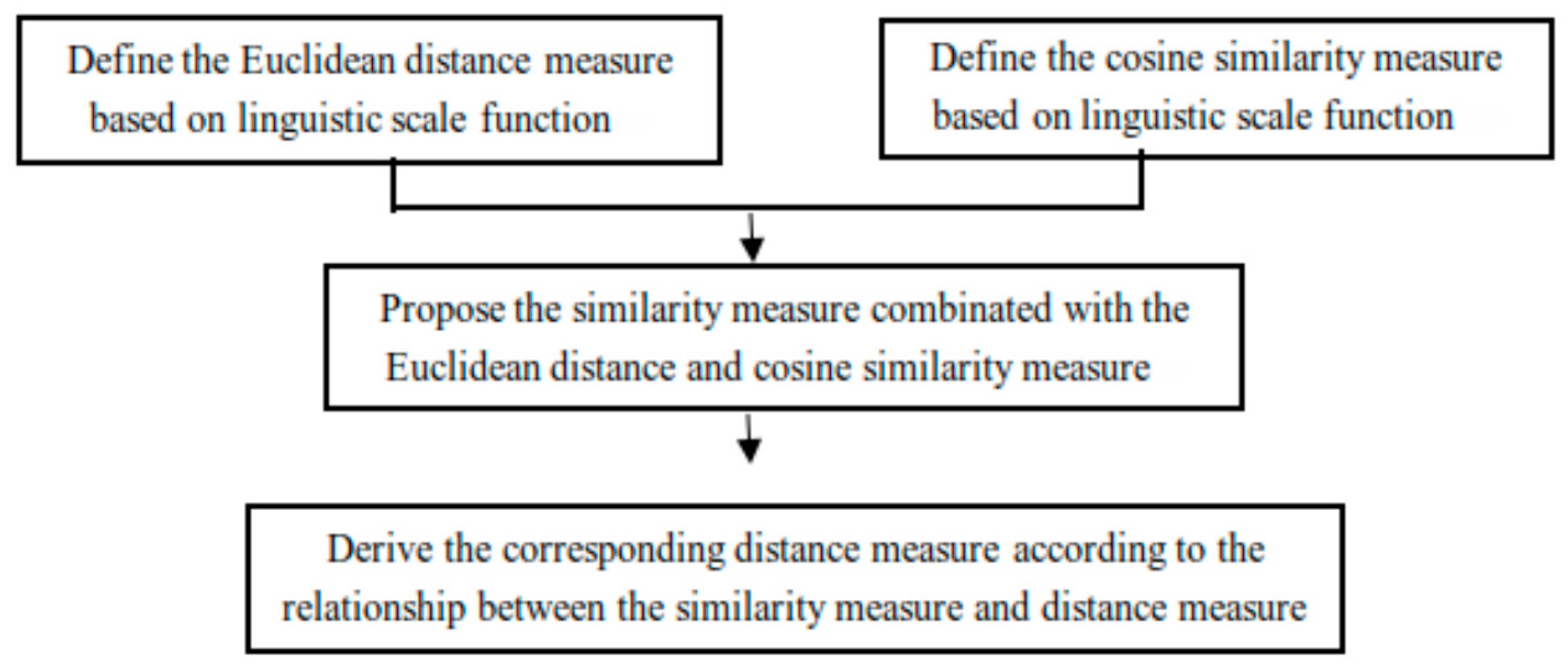[31] used the subscript of linguistic terms directly in the process of operations; they did not consider the semantic environment, which may cause the loss of information in the decision process. In order to overcome its disadvantages, next we will construct a new similarity measure and derive a corresponding distance measure. A scheme of this process is shown in Figure 2.

At first, we improve the existing distance measure (1) and similarity measure (2) based on a linguistic scale function, which can be defined as follows:

Definition 8.

Given a fixed set$X$, let$S=\{s_i|i=0,1,\cdots ,2t\}$be a LTS, and let$f$be a linguistic scale function,$h_S^k\left(x_j\right)=\{s_{{\delta }_l^k}\left(x_j\right)|s_{{\delta }_l^k}\left(x_j\right)\in S,l=1,2,\cdots ,L_j\}$, where$L_j=max\{l\left(h_S^1\left(x_j\right),l(h_S^2\left(x_j\right)\right)\}$,$l\left(h_S^k\left(x_j\right)\right)$represents the number of elements in$h_S^k\left(x_j\right)$$\left(k=1,2\right)$. For any two HFLTSs$H_S^1=\{(x_j,$$h_S^1\left(x_j\right))|x_j\in X\}$and$H_S^2=\{\left(x_j,h_S^2\left(x_j\right)\right)|x_j\in X\}\left(j=1,2,\cdots ,n\right)$, if the weight of the different element$x_j$is${\omega }_j\left(j=1,2,\cdots ,n\right)$, then the improved weighted distance measure between HFLTSs$H_S^1$and$H_S^2$can be defined as follows:

$$D_{\omega HFL}^{\prime }\left(H_S^1,H_S^2\right)={\left({\displaystyle {\displaystyle \sum }_{j=1}^n}\frac{{\omega }_j}{L_j}{\displaystyle {\displaystyle \sum }_{l=1}^{L_j}}{\left(\left|f\left(s_{{\delta }_l^1}\left(x_j\right)\right)-f\left(s_{{\delta }_l^2}\left(x_j\right)\right)\right|\right)}^2\right)}^{\frac{1}{2}}.$$

Theorem 2.

Let$H_S^1$and$H_S^2$be any two HFLTSs, and let$f$be a linguistic scale function; the distance measure$D_{\omega HFL}^{\prime }$between HFLTSs satisfies the following properties:

(1) 

$0\le D_{\omega HFL}^{\prime }\left(H_S^1,H_S^2\right)\le 1$;

(2) 

$D_{\omega HFL}^{\prime }\left(H_S^1,H_S^2\right)=0$if and only if$H_S^1=H_S^2$;

(3) 

$D_{\omega HFL}^{\prime }\left(H_S^1,H_S^2\right)=D_{\omega HFL}^{\prime }\left(H_S^2,H_S^1\right)$.

Proof. 

Properties (1), (2), and (3) are obvious, and we omit the proof here. ☐

Remark 4.

For all$j=1,2,\cdots ,n$, if the weight${\omega }_j=\frac{1}{n}$, then the improved weighted distance measure$D_{\omega HFL}^{\prime }\left(H_S^1,H_S^2\right)$is reduced to the improved Euclidean distance measure$D_{HFL}^{\prime }\left(H_S^1,H_S^2\right)$:

$$D_{HFL}^{\prime }\left(H_S^1,H_S^2\right)={\left(\frac{1}{n}\left({\displaystyle {{\displaystyle \sum }}_{j=1}^n}\frac{1}{L_j}{\displaystyle {{\displaystyle \sum }}_{l=1}^{L_j}}{\left(\left|f\left(s_{{\delta }_l^1}\left(x_j\right)\right)-f\left(s_{{\delta }_l^2}\left(x_j\right)\right)\right|\right)}^2\right)\right)}^{\frac{1}{2}}.$$

Definition 9.

Given a fixed set$X$, let$S=\{s_i|i=0,1,\cdots ,2t\}$be a LTS, and let$f$be a linguistic scale function,$h_S^k\left(x_j\right)=\{s_{{\delta }_l^k}\left(x_j\right)|s_{{\delta }_l^k}\left(x_j\right)\in S,l=1,2,\cdots ,L_j\}$, where$L_j=max\{l\left(h_S^1\left(x_j\right),l(h_S^2\left(x_j\right)\right)\}$,$l\left(h_S^k\left(x_j\right)\right)$represents the number of elements in$h_S^k\left(x_j\right)$$\left(k=1,2\right)$. For any two HFLTSs$H_S^1=\{(x_j,$$h_S^1\left(x_j\right))|x_j\in X\}$and$H_S^2=\{\left(x_j,h_S^2\left(x_j\right)\right)|x_j\in X\}\left(j=1,2,\cdots ,n\right)$, if the weight of different element$x_j$is${\omega }_j\left(j=1,2,\cdots ,n\right)$, then the improved weighted cosine similarity measure between$H_S^1$and$H_S^2$can be defined as:

$$Co{s}_{\omega HFL}^{\prime }\left(H_S^1,H_S^2\right)=\frac{{{\displaystyle \sum }}_{j=1}^n\left(\frac{{\omega }_j}{L_j}{{\displaystyle \sum }}_{l=1}^{L_j}f\left(s_{{\delta }_l^1}\left(x_j\right)\right)·f\left(s_{{\delta }_l^2}\left(x_j\right)\right)\right)}{{\left({{\displaystyle \sum }}_{j=1}^n\left(\frac{{\omega }_j}{L_j}{{\displaystyle \sum }}_{l=1}^{L_j}{\left(f\left(s_{{\delta }_l^1}\left(x_j\right)\right)\right)}^2\right)·{{\displaystyle \sum }}_{j=1}^n\left(\frac{{\omega }_j}{L_j}{{\displaystyle \sum }}_{l=1}^{L_j}{\left(f\left(s_{{\delta }_l^2}\left(x_j\right)\right)\right)}^2\right)\right)}^{\frac{1}{2}}}.$$

Remark 5.

For all$j=1,2,\cdots ,n$, if the weight${\omega }_j=\frac{1}{n}$, then the improved weighted cosine similarity measure$Co{s}_{\omega HFL}^{\prime }\left(H_S^1,H_S^2\right)$is reduced to the similarity measure$Co{s}_{HFL}^{\prime }\left(H_S^1,H_S^2\right)$:

$$Co{s}_{HFL}^{\prime }\left(H_S^1,H_S^2\right)=\frac{{{\displaystyle \sum }}_{j=1}^n\left(\frac{1}{L_j}{{\displaystyle \sum }}_{l=1}^{L_j}f\left(s_{{\delta }_l^1}\left(x_j\right)\right)·f\left(s_{{\delta }_l^2}\left(x_j\right)\right)\right)}{{\left({{\displaystyle \sum }}_{j=1}^n\left(\frac{1}{L_j}{{\displaystyle \sum }}_{l=1}^{L_j}{\left(f\left(s_{{\delta }_l^1}\left(x_j\right)\right)\right)}^2\right)·{{\displaystyle \sum }}_{j=1}^n\left(\frac{1}{L_j}{{\displaystyle \sum }}_{l=1}^{L_j}{\left(f\left(s_{{\delta }_l^2}\left(x_j\right)\right)\right)}^2\right)\right)}^{\frac{1}{2}}}.$$

In the following, we go on to propose a similarity measure between the HFLTSs, which combine the distance measure $D_{HFL}^{\prime }$ and the cosine similarity measure ${Cos}_{HFL}^{\prime }$.

Definition 10.

Given a fixed set$X$, let$S=\{s_i|i=0,1,\cdots ,2t\}$be a LTS, and let$f$be a linguistic scale function,$h_S^k\left(x_j\right)=\{s_{{\delta }_l^k}\left(x_j\right)|s_{{\delta }_l^k}\left(x_j\right)\in S,l=1,2,\cdots ,L_j\}$, where$L_j=max\{l(h_S^1\left(x_j\right)$,$l(h_S^2\left(x_j\right))\}$,$l\left(h_S^k\left(x_j\right)\right)$represents the number of elements in$h_S^k\left(x_j\right)$$\left(k=1,2\right)$. For any two HFLTSs$H_S^1=\{(x_j,$$h_S^1\left(x_j\right))|x_j\in X\}$and$H_S^2=\{\left(x_j,h_S^2\left(x_j\right)\right)|x_j\in X\}\left(j=1,2,\cdots ,n\right)$, then the new similarity measure$S_{HFL}^{\ast }\left(H_S^1,H_S^2\right)$can be defined as follows:

$$S_{HFL,}^{\ast }\left(H_S^1,H_S^2\right)=\frac{1}{2}\left(Co{s}_{HFL}^{\prime }\left(H_S^1,H_S^2\right)+1-D_{HFL}^{\prime }\left(H_S^1,H_S^2\right)\right)$$

where$Co{s}_{HFL}^{\prime }\left(H_S^1,H_S^2\right)=\frac{{{\displaystyle \sum }}_{j=1}^n\left(\frac{1}{L_j}{{\displaystyle \sum }}_{l=1}^{L_j}f\left(s_{{\delta }_l^1}\left(x_j\right)\right)·f\left(s_{{\delta }_l^2}\left(x_j\right)\right)\right)}{{\left({{\displaystyle \sum }}_{j=1}^n\left(\frac{1}{L_j}{{\displaystyle \sum }}_{l=1}^{L_j}{\left(f\left(s_{{\delta }_l^1}\left(x_j\right)\right)\right)}^2\right)·{{\displaystyle \sum }}_{j=1}^n\left(\frac{1}{L_j}{{\displaystyle \sum }}_{l=1}^{L_j}{\left(f\left(s_{{\delta }_l^2}\left(x_j\right)\right)\right)}^2\right)\right)}^{\frac{1}{2}}}$, $D_{HFL}^{\prime }\left(H_S^1,H_S^2\right)={\left(\frac{1}{n}\left({\displaystyle {{\displaystyle \sum }}_{j=1}^n}\frac{1}{L_j}{\displaystyle {{\displaystyle \sum }}_{l=1}^{L_j}}{\left(\left|f\left(s_{{\delta }_l^1}\left(x_j\right)\right)-f\left(s_{{\delta }_l^2}\left(x_j\right)\right)\right|\right)}^2\right)\right)}^{\frac{1}{2}}$.

Theorem 3.

The similarity measure$S^{\ast }\left(H_S^1,H_S^2\right)$is a regular similarity measure.

Proof. 

According to Lemma 2, we will prove it by three steps as follows:

(1)

Since $0\le f\le 1,Co{s}_{HFL}^{\prime }\left(H_S^1,H_S^2\right)$ can be considered as the extension of cosine function, then $0\le Co{s}_{HFL}^{\prime }\left(H_S^1,H_S^2\right)\le 1$. According to Theorem 2, we know that $D_{HFL}^{\prime }\left(H_S^1,H_S^2\right)$ is a distance measure, then $0\le 1-D_{HFL}^{\prime }\left(H_S^1,H_S^2\right)\le 1$. Thus, we get $0\le Co{s}_{HFL}^{\prime }\left(H_S^1,H_S^2\right)+1-D_{HFL}^{\prime }\left(H_S^1,H_S^2\right)\le 2$, so $0\le S_{HFL}^{\ast }\left(H_S^1,H_S^2\right)\le 1$ is obvious.

(2)

If $H_S^1=H_S^2$, we have $f(s_{{\delta }_l^1}\left(x_j\right))=f(s_{{\delta }_l^2}\left(x_j\right))$, $Co{s}_{HFL}^{\prime }\left(H_S^1,H_S^2\right)=1$, $D_{HFL}^{\prime }\left(H_S^1,H_S^2\right)=0$, then $S_{HFL}^{\ast }\left(H_S^1,H_S^2\right)=1$. On the other hand, when $S_{HFL}^{\ast }\left(H_S^1,H_S^2\right)=1$, we have $Co{s}_{HFL}^{\prime }\left(H_S^1,H_S^2\right)+1-D_{HFL}^{\prime }\left(H_S^1,H_S^2\right)=2$; that is, $Co{s}_{HFL}^{\prime }\left(H_S^1,H_S^2\right)=1+D_{HFL}^{\prime }\left(H_S^1,H_S^2\right)$. Because $0\le Co{s}_{HFL}^{\prime }\left(H_S^1,H_S^2\right)\le 1$, $D_{HFL}^{\prime }\left(H_S^1,H_S^2\right)\ge 0$ hold simultaneously, then we have $D_{HFL}^{\prime }\left(H_S^1,H_S^2\right)=0$, $Co{s}_{HFL}^{\prime }\left(H_S^1,H_S^2\right)=1$. When $Co{s}_{HFL}^{\prime }\left(H_S^1,H_S^2\right)=1$, we know that $H_S^1=k{H}_S^2$ and $k$ is a constant; while $D_{HFL}^{\prime }\left(H_S^1,H_S^2\right)=0$, we know that $H_S^1=H_S^2$. That is to say, when $S_{HFL}^{\ast }\left(H_S^1,H_S^2\right)=1$, $H_S^1=H_S^2$.

Thus, $S_{HFL}^{\ast }\left(H_S^1,H_S^2\right)=1$ if and only if $H_S^1=H_S^2$.

(3)

According to Remark 5, $Co{s}_{HFL}^{\prime }\left(H_S^1,H_S^2\right)=Co{s}_{HFL}^{\prime }\left(H_S^2,H_S^1\right)$ is obvious. From Theorem 2, it is already known that when $D_{HFL}^{\prime }\left(H_S^1,H_S^2\right)=D_{HFL}^{\prime }\left(H_S^2,H_S^1\right)$, then $S_{HFL}^{\ast }\left(H_S^1,H_S^2\right)=S_{HFL}^{\ast }\left(H_S^2,H_S^1\right)$ are proven. ☐

From Theorem 3, we know that the proposed similarity measure $S_{HFL}^{\ast }$ is a regular similarity measure, which overcomes the disadvantages of the similarity measure as defined by Liao et al. [31].

Remark 6.

According to the relation between the distance measure and the regular similarity measure, we can obtain a new distance measure$D_{HFL}^{\ast }\left(H_S^1,H_S^2\right)$, which is based on the proposed similarity measure$S_{HFL}^{\ast }\left(H_S^1,H_S^2\right)$:

$$\begin{array}{l}{D}_{HFL}^{\ast }\left(H_S^1,H_S^2\right)=1-S_{HFL}^{\ast }\left(H_S^1,H_S^2\right)=\frac{1}{2}\left(1-Co{s}_{HFL}^{\prime }\left(H_S^1,H_S^2\right)+D_{HFL}^{\prime }\left(H_S^1,H_S^2\right)\right)\\ =\frac{1}{2}(1-\frac{{{\displaystyle \sum }}_{j=1}^n\left(\frac{1}{L_j}{{\displaystyle \sum }}_{l=1}^{L_j}f\left(s_{{\delta }_l^1}\left(x_j\right)\right)·f\left(s_{{\delta }_l^2}\left(x_j\right)\right)\right)}{{\left({{\displaystyle \sum }}_{j=1}^n\left(\frac{1}{L_j}{{\displaystyle \sum }}_{l=1}^{L_j}{\left(f\left(s_{{\delta }_l^1}\left(x_j\right)\right)\right)}^2\right)·{{\displaystyle \sum }}_{j=1}^n\left(\frac{1}{L_j}{{\displaystyle \sum }}_{l=1}^{L_j}{\left(f\left(s_{{\delta }_l^2}\left(x_j\right)\right)\right)}^2\right)\right)}^{\frac{1}{2}}}+{\left(\frac{1}{n}\left({\displaystyle {{\displaystyle \sum }}_{j=1}^n}\frac{1}{L_j}{\displaystyle {{\displaystyle \sum }}_{l=1}^{L_j}}{\left(\left|f\left(s_{{\delta }_l^1}\left(x_j\right)\right)-f(s_{{\delta }_l^2}\left(x_j\right))\right|\right)}^2\right)\right)}^{\frac{1}{2}}).\end{array}$$

Theorem 4.

The new distance measure$D_{HFL}^{\ast }\left(H_S^1,H_S^2\right)$satisfies the following properties:

(1) 

$0\le D_{HFL}^{\ast }\left(H_S^1,H_S^2\right)\le 1$;

(2) 

$D_{HFL}^{\ast }\left(H_S^1,H_S^2\right)=0$if and only if$H_S^1=H_S^2$;

(3) 

$D_{HFL}^{\ast }\left(H_S^1,H_S^2\right)=D_{HFL}^{\ast }\left(H_S^2,H_S^1\right)$.

Proof. 

Properties (1) and (3) are obvious, here we only present the proof of property (2).

If $H_S^1=H_S^2$, we have $S_{HFL}^{\ast }\left(H_S^1,H_S^2\right)=1$, then $D_{HFL}^{\ast }\left(H_S^1,H_S^2\right)=1-S_{HFL}^{\ast }\left(H_S^1,H_S^2\right)=0$. On the other hand, when $D_{HFL}^{\ast }\left(H_S^1,H_S^2\right)=0$, we have $S_{HFL}^{\ast }\left(H_S^1,H_S^2\right)=1-D_{HFL}^{\ast }\left(H_S^1,H_S^2\right)=1$. Because $S_{HFL}^{\ast }$ is a regular similarity measure, according to Lemma 2, we have $H_S^1=H_S^2$.

Thus, we obtain $D_{HFL}^{\ast }\left(H_S^1,H_S^2\right)=0$ if and only if $H_S^1=H_S^2$. ☐

Definition 11.

Given a fixed set$X$, let$S=\{s_i|i=0,1,\cdots ,2t\}$be a LTS, and let$f$be a linguistic scale function.$h_S^k\left(x_j\right)=\{s_{{\delta }_l^k}\left(x_j\right)|s_{{\delta }_l^k}\left(x_j\right)\in S,l=1,2,\cdots ,L_j\}$, where$L_j=max\{l(h_S^1\left(x_j\right)$,$l(h_S^2\left(x_j\right))\}$,$l\left(h_S^k\left(x_j\right)\right)$represents the number of elements in$h_S^k\left(x_j\right)$$\left(k=1,2\right)$. For any two HFLTSs$H_S^1=\{(x_j,$$h_S^1\left(x_j\right))|x_j\in X\}$and$H_S^2=\{\left(x_j,h_S^2\left(x_j\right)\right)|x_j\in X\}\left(j=1,2,\cdots ,n\right)$, the associated weighting vector$\omega =\left({\omega }_1,{\omega }_2,\cdots ,{\omega }_j\right)$satisfying with${\displaystyle {{\displaystyle \sum }}_{j=1}^n}{\omega }_j=1\left(0\le {\omega }_j\le 1\right)$, then the weighted similarity measure between$H_S^1$and$H_S^2$can be defined as:

$$S_{\omega HFL}^{\ast }\left(H_S^1,H_S^2\right)=\frac{1}{2}\left(Co{s}_{\omega HFL}^{\prime }\left(H_S^1,H_S^2\right)+1-D_{\omega HFL}^{\prime }\left(H_S^1,H_S^2\right)\right)$$

Theorem 5.

The weighted similarity measure$S_{\omega HFL}^{\ast }\left(H_S^1,H_S^2\right)$is also a regular similarity measure.

Proof. 

The proof is similar to Theorem 3; we omit it here. ☐

Remark 7.

If the weight of the different element$x_j$is${\omega }_j\left(j=1,2,\cdots ,n\right)$, satisfying${\displaystyle {{\displaystyle \sum }}_{j=1}^n}{\omega }_j=1\left(0\le {\omega }_j\le 1\right)$, then the weighted distance measure between$H_S^1$and$H_S^2$can be obtained by:

$$D_{\omega HFL}^{\ast }\left(H_S^1,H_S^2\right)=1-S_{\omega HFL}^{\ast }\left(H_S^1,H_S^2\right)$$

Remark 8.

If we take the weight${\omega }_j=\frac{1}{n}\left(j=1,2,\cdots ,n\right)$in$S_{\omega HFL}^{\ast }\left(H_S^1,H_S^2\right)$and$D_{\omega HFL}^{\ast }\left(H_S^1,H_S^2\right)$, then$S_{\omega HFL}^{\ast }\left(H_S^1,H_S^2\right)$and$D_{\omega HFL}^{\ast }\left(H_S^1,H_S^2\right)$are reduced to$S_{HFL}^{\ast }\left(H_S^1,H_S^2\right)$and$D_{HFL}^{\ast }\left(H_S^1,H_S^2\right)$, respectively.

Next, we utilize the medical diagnosis example to illustrate the application of the proposed similarity measure.

Example 5.

In traditional Chinese medical diagnosis, doctors diagnose patients by watching, smelling, asking and touching, so the doctor always get some imprecise information about patients’ symptoms. Let us consider a set of diagnoses$G=\{Viralfever,Typhoid,Pneumonia,Stomachproblem\}$and a set of symptoms$X=\{temperature,headache,cough,stomachpain$}. Assume that a patient, with respect to all symptoms, can be depicted as the following LTS, respectively:$S_1=\{s_0:verylow,s_1:low,s_2:slightly$low,$s_3:normal,s_4:slightlyhigh,s_5:high,s_6:veryhigh\},S_j=\{s_0:none,s_1:veryslight,s_2:$$slight,s_3:normal,s_4:slightlyterrible,s_5:terrible,s_6:veryterrible\}\left(j=2,3,4\right)$. Furthermore, let${\omega }_j=$$\left(0.25,0.25,0.25,0.25\right)\left(j=1,2,3,4\right)$be the weight vector of symptoms.

Suppose that the patient $P=\{Richard,Catherine,Nicle,Kevin\}$ has all of the symptoms, which are represented by a HFLTS and are given in

Table 1. Symptoms characteristic for the patients.

	Viral Fever	Typhoid	Pneumonia	Stomach Problem
Richard	{s5}	{s5}	{s4,s5}	{s0}
Catherine	{s3}	{s0}	{s0}	{s4,s5}
Nicle	{s6}	{s4}	{s5}	{s0}
Kevin	{s4}	{s2,s3}	{s5}	{s0}

.

According to experience, each patient’s symptoms diagnosis can be viewed as a HFLTS, and these are shown in

Table 2. Symptoms characteristic for the diagnosis.

	Viral Fever	Typhoid	Pneumonia	Stomach Problem
Richard	{s4,s5,s6}	{s3,s4,s5}	{s4,s5,s6}	{s0}
Catherine	{s5,s6}	{s1,s2,s3}	{s4,s5,s6}	{s0,s1}
Nicle	{s3,s4}	{s2,s3}	{s5,s6}	{s0}
Kevin	{s3}	{s0}	{s0}	{s4,s5,s6}

.

In order to diagnose what kind of symptoms that the patients belong to, we can calculate the similarity measure between each patient’s symptoms and the diagnosis. If the linguistic scale function $f=f_1\left(s_i\right)=\frac{i}{2t}\left(t=3\right)$, we apply the proposed similarity measure $S_{\omega HFL}^{\ast }$ to calculate the degree of similarity between each patient’s symptoms and the diagnosis; the results are shown in

Table 3. Hesitant fuzzy linguistic similarity measure.

	Viral Fever	Typhoid	Pneumonia	Stomach Problem
Richard	0.9574	0.9702	0.8973	0.8606
Catherine	0.7865	0.7856	0.8323	0.9954
Nicle	0.9558	0.9517	0.8846	0.7741
Kevin	0.9279	0.8728	0.9814	0.8370

.

It is already known that the larger value of similarity measure, the higher the possibility of diagnosis for the patient. From the above results of Table 3, the symptoms of Richard, Catherine, Nicole, and Kevin indicate that they are suffering from typhoid, stomach problems, viral fever, and pneumonia, respectively.

4. The TOPSIS Method with the Proposed Distance Measure ${\mathit{D}}_{\mathit{\omega }\mathit{H}\mathit{F}\mathit{L}}^{\mathbf{\ast }}$

In Section 4, we will present the TOPSIS method [40] to the proposed distance measure ${\mathrm{D}}_{\mathsf{\omega }\mathrm{HFL}}^{\ast }$ for hesitant fuzzy linguistic multi-criteria decision-making problems.

Suppose that a panel of decision makers are invited to evaluate the alternatives $H=\{H_1,H_2,\cdots ,H_m\}$ with respect to the criteria $C=\{C_1,C_2,\cdots ,C_n\}$. Let $S=\{s_i|i=0, 1,\cdots ,2t\}$ be a LTS, let ${\omega }_j$ $\left(j=1,2,\cdots ,n\right)$ be the weight of criteria $C_j$, where $0\le {\omega }_j\le 1$ $\left(j=1, 2,\cdots ,n\right)$ and ${\displaystyle {{\displaystyle \sum }}_{j=1}^n}{\omega }_j=1$; the hesitant fuzzy linguistic information decision matrix $H$ are given as follows:

$$H=\left(\begin{array}{cccc}{H}_S^{11}& H_S^{12}& \cdots & H_S^{1n}\\ H_S^{21}& H_S^{22}& \cdots & H_S^{2n}\\ ⋮& ⋮& \ddots & ⋮\\ H_S^{m1}& H_S^{m2}& \cdots & H_S^{mn}\end{array}\right),$$

where $H_S^{ij}=\{s_{{\delta }_l}^{ij}|l=1,2,\cdots , L_j\}\left(i=1, 2,\cdots , m;j=1,2,\cdots ,n\right)$ are HFLTSs, representing the evaluation about alternative $H_i$ with respect to the criterion $C_j$.

Next, we present the TOPSIS method with the distance measure $D_{\omega HFL}^{\ast }$ for MCDM problems. In general, it includes the following steps:

Step 1. Normalize the hesitant fuzzy linguistic decision matrix $H$.

If the criteria belong to the benefit-type, we need not do anything; if the criteria belong to the cost-type, we should use $neg\left(s_i\right)=s_j\left(i+j=2t\right)$ to normalize the decision matrix.

Step 2. For $i=1, 2,\cdots ,m,j=1, 2,\cdots ,n$, the hesitant fuzzy linguistic positive ideal solution (HFLPIS) $H^{+}=\{H_S^{1+},H_S^{2+},\cdots ,H_S^{n+}\}$ and hesitant fuzzy linguistic negative ideal solution (HFLNIS) ${\mathrm{H}}^{-}=\{{\mathrm{H}}_{\mathrm{S}}^{1-},{\mathrm{H}}_{\mathrm{S}}^{2-},\cdots ,{\mathrm{H}}_{\mathrm{S}}^{\mathrm{n}-}\}$ are given in the following:

$$H_S^{j+}=H_S^{ij},H_S^{j-}=H_S^{ij}.$$

For criteria $C_j\left(j=1, 2,\cdots ,n\right)$, by the score function proposed in Definition 7, we can get the value of $F^{\ast }(H_S^{ij}) \left(i=1, 2,\cdots ,m\right)$. According to Theorem 1, the order relationship for HFLTSs can be given as: if $F^{\ast }\left(H_S^1\right)>F^{\ast }\left(H_S^2\right)$, then $H_S^1>H_S^2$, so that $H_S^{j+}$ and $H_S^{j-}$ can be obtained.

Step 3. Use the distance measure to calculate the separation of each alternative between the HFLPIS $H^{+}=\{H_S^{1+},H_S^{2+},\cdots ,H_S^{n+}\}$ and HFLNIS $H^{-}=\{H_S^{1-},H_S^{2-},\cdots ,H_S^{n-}\}$, respectively.

The distance measure between $H_i\left(i=1, 2,\cdots ,m\right)$ and $H^{+}$ can be given as: $D_i^{+}={\displaystyle {{\displaystyle \sum }}_{j=1}^n}{D}_{\omega HFL}^{\ast }(H_S^{ij},H^{+})$. Similarly to the distance measure $D_i^{+}$, the distance measure between the alternative $H_i\left(i=1, 2,\cdots ,m\right)$ and $H^{-}$ is obtained as: $D_i^{-}={\displaystyle {{\displaystyle \sum }}_{j=1}^n}{D}_{\omega HFL}^{\ast }(H_S^{ij},H^{-})$.

For the given $H_i\left(i=1,2,\cdots ,m\right)$,

$$\begin{array}{l}{D}_i^{+}={\displaystyle {{\displaystyle \sum }}_{j=1}^n}{D}_{\omega HFL}^{\ast }(H_S^{ij},H^{+})={\displaystyle {{\displaystyle \sum }}_{j=1}^n}(1-\frac{1}{2}(Co{s}_{\omega HFL}^{\prime }(H_S^{ij},H^{+})+1-D_{\omega HFL}^{\prime }(H_S^{ij},H^{+})))={\displaystyle {{\displaystyle \sum }}_{j=1}^n}\frac{1}{2}(1-\\ Co{s}_{\omega HFL}^{\prime }\left(H_S^{ij},H^{+}\right)+D_{\omega HFL}^{\prime }\left(H_S^{ij},H^{+}\right) )={\displaystyle {{\displaystyle \sum }}_{j=1}^n}\frac{1}{2}(1-\frac{{{\displaystyle \sum }}_{j=1}^n\left(\frac{1}{L_j}{{\displaystyle \sum }}_{l=1}^{L_j}f\left(s_{{\delta }_l^{ij}}\left(x_j\right)\right)·f\left(s_{{\delta }_l^{+}}\left(x_j\right)\right)\right)}{{\left({{\displaystyle \sum }}_{j=1}^n\left(\frac{1}{L_j}{{\displaystyle \sum }}_{l=1}^{L_j}{\left(f\left(s_{{\delta }_l^{ij}}\left(x_j\right)\right)\right)}^2\right)·{{\displaystyle \sum }}_{j=1}^n\left(\frac{1}{L_j}{{\displaystyle \sum }}_{l=1}^{L_j}{\left(f\left(s_{{\delta }_l^{+}}\left(x_j\right)\right)\right)}^2\right)\right)}^{\frac{1}{2}}}+\\ {\left({\displaystyle {{\displaystyle \sum }}_{j=1}^n}\frac{{\omega }_j}{L_j}{\displaystyle {{\displaystyle \sum }}_{l=1}^{L_j}}{\left(\left|f\left(s_{{\delta }_l^{ij}}\left(x_j\right)\right)-f\left(s_{{\delta }_l^{+}}\left(x_j\right)\right)\right|\right)}^2\right)}^{\frac{1}{2}});\end{array}$$

$$\begin{array}{l}{D}_i^{-}={\displaystyle {{\displaystyle \sum }}_{j=1}^n}{D}_{\omega HFL}^{\ast }\left(H_S^{ij},H^{-}\right)={\displaystyle {{\displaystyle \sum }}_{j=1}^n}\left(1-\frac{1}{2}\left(Co{s}_{\omega HFL}^{\prime }\left(H_S^{ij},H^{-}\right)+1-D_{\omega HFL}^{\prime }\left(H_S^{ij},H^{-}\right)\right)\right)={\displaystyle {{\displaystyle \sum }}_{j=1}^n}\frac{1}{2}(1-\\ Co{s}_{\omega HFL}^{\prime }\left(H_S^{ij},H^{-}\right)+D_{\omega HFL}^{\prime }\left(H_S^{ij},H^{-}\right) )={\displaystyle {{\displaystyle \sum }}_{j=1}^n}\frac{1}{2}(1-\frac{{{\displaystyle \sum }}_{j=1}^n\left(\frac{1}{L_j}{{\displaystyle \sum }}_{l=1}^{L_j}f\left(s_{{\delta }_l^{ij}}\left(x_j\right)\right)·f\left(s_{{\delta }_l^{-}}\left(x_j\right)\right)\right)}{{\left({{\displaystyle \sum }}_{j=1}^n\left(\frac{1}{L_j}{{\displaystyle \sum }}_{l=1}^{L_j}{\left(f\left(s_{{\delta }_l^{ij}}\left(x_j\right)\right)\right)}^2\right)·{{\displaystyle \sum }}_{j=1}^n\left(\frac{1}{L_j}{\displaystyle {{\displaystyle \sum }}_{l=1}^{L_j}}{\left(f\left(s_{{\delta }_l^{-}}\left(x_j\right)\right)\right)}^2\right)\right)}^{\frac{1}{2}}}+\\ {\left({\displaystyle {{\displaystyle \sum }}_{j=1}^n}\frac{{\omega }_j}{L_j}{\displaystyle {{\displaystyle \sum }}_{l=1}^{L_j}}{\left(\left|f\left(s_{{\delta }_l^{ij}}\left(x_j\right)\right)-f\left(s_{{\delta }_l^{-}}\left(x_j\right)\right)\right|\right)}^2\right)}^{\frac{1}{2}}).\end{array}$$

Step 4. Calculate the closeness coefficient ${\mathsf{\Phi }}_i$ of each alternative $H_i\left(i=1, 2,\cdots ,m\right)$:

$${\mathsf{\Phi }}_i=\frac{D_i^{-}}{D_i^{+}+D_i^{-}}.$$

Step 5. Rank the alternatives by decreasing order of the closeness coefficient ${\mathsf{\Phi }}_i$; the greater value ${\mathsf{\Phi }}_i$ is, the better alternative $H_i$ will be.

5. Numerical Example

In this section, we give a numerical example that concerns logistics outsourcing (adapted from Wang et al. [38]) to illustrate the feasibility of the TOPSIS method with the proposed distance measure $D_{\omega HFL}^{\ast }$.

5.1. Background

The ABC Limited Company is a passenger car manufacturer in China. To improve the competitiveness of products and reduce production costs, ABC decides to choose a third-party logistics service provider for logistics outsourcing. Through preliminary selection, five possible logistics providers $H=\{H_1,H_2,H_3,H_4,H_5\}$ are provided for further evaluation with respect to the following four criteria: service ($C_1$), relationship ($C_2$), quality ($C_3$), and equipment systems ($C_4$). Furthermore, assume that the weight vector of criteria $C_j$ ($j=$1, 2, 3, 4) is $\mathsf{\omega }=\left(0.4,0.3,0.2,0.1\right)$. Three experts with different backgrounds are invited by the company to evaluate the TPLSP. Since these criteria are all qualitative, it is suitable for the experts to express their views in linguistic term sets. The ABC Company uses a LTS of seven terms to evaluate the TPLSP, which can be expressed by $S=\{s_0:very poor,s_1:poor, s_2:slightly poor,s_3:fair,s_4:slightly good, s_5:good,s_6:very good\}$. The final judgment of the five providers with the hesitant fuzzy linguistic decision matrix $H={(H_S^{ij})}_{5\times 4}$ are given in

Table 4. The hesitant fuzzy linguistic decision matrix provided by experts.

	${\mathit{C}}_1$	${\mathit{C}}_2$	${\mathit{C}}_3$	${\mathit{C}}_4$
$H_1$	{s2,s3,s4}	{s3,s6}	{s4,s6}	{s0,s1,s2}
$H_2$	{s3,s4}	{s4,s6}	{s0,s1}	{s1,s4}
$H_3$	{s0,s1}	{s4}	{s0,s1,s3}	{s2}
$H_4$	{s5}	{s1,s3}	{s4,s6}	{s0,s1,s4}
$H_5$	{s4,s5}	{s2,s3}	{s1,s3,s4}	{s0,s2}

.

To verify the feasibility and effectiveness of the decision method proposed in Section 4, at first, we assume $f=f_1\left(s_i\right)=\frac{i}{2t} \left(t=3\right)$.

Step 1. Normalize the hesitant fuzzy linguistic decision matrix.

It is already known the criteria $C_1,C_2,C_3,C_4$ are all benefit-type criteria, and thus we do not need to do anything.

Step 2. According to the score function in Theorem 1, we can calculate the HFLPIS ${\mathrm{H}}^{+}$ and the HFLNIS ${\mathrm{H}}^{-}$, which are given as follows:

$$H^{+}=\{\{s_5\},\{s_4,s_6\},\{s_4,s_6\},\{s_1,s_4\}\}$$

$$H^{-}=\{\{s_0, s_1\},\{s_1, s_3\},\{s_0,s_1,s_3\},\{s_0, s_2\}\}$$

Step 3. Calculate the distance measure $D_{\omega HFL}^{\ast }(H_S^{ij},H^{+})$ and $D_{\omega HFL}^{\ast }(H_S^{ij},H^{-})$ for different alternative $H_i\left(i=1,2,3,4,5\right)$ respectively, which are given in

Table 5. The distance measure of each alternative.

	${\mathit{D}}_{\mathit{i}}^{+}$	${\mathit{D}}_{\mathit{i}}^{-}$
$H_1$	0.1524	0.2907
$H_2$	0.2395	0.3169
$H_3$	0.4201	0.1694
$H_4$	0.1753	0.4624
$H_5$	0.1884	0.3740

.

Step 4. Calculate the closeness coefficient ${\mathsf{\Phi }}_i$ of each alternative $H_i$; they are obtained in

Table 6. The closeness coefficient of each alternative.

	${\mathit{H}}_1$	${\mathit{H}}_2$	${\mathit{H}}_3$	${\mathit{H}}_4$	${\mathit{H}}_5$
${\mathsf{\Phi }}_i$	0.6561	0.5695	0.2873	0.7251	0.6650

.

Step 5. Rank the alternatives $H_i$ and utilize ${\mathsf{\Phi }}_i \left(i=1, 2, 3, 4, 5\right)$.

It is already known that $H_4\succ H_5\succ H_1\succ H_2\succ H_3$, which means that the best choice is $H_4$.

In order to illustrate the impact of the linguistic scale function $f$ on MCDM, we use the different linguistic scale functions $f=f_2\left(s_i\right) \left(a=1.4,t=3\right)$ and $f=f_3\left(s_i\right) \left(\alpha =\beta =0.8\right)$ to calculate the distance measure between HFLTSs, the results are given in

Table 7. Results obtained by different linguistic scale functions.

	Ranking
$f=f_1\left(s_i\right)$	$H_4\succ H_5\succ H_1\succ H_2\succ H_3$
$f=f_2\left(s_i\right)$	$H_4\succ H_1\succ H_5\succ H_2\succ H_3$
$f=f_3\left(s_i\right)$	$H_4\succ H_5\succ H_1\succ H_2\succ H_3$

.

The results between the different linguistic scale functions are shown in Figure 3.

5.2. Comparison Analysis

To illustrate the feasibility and effectiveness of the proposed method, different approaches are used to compare with the same numerical example. The comparison is displayed in

Table 8. Comparison of different methods.

	Ranking
Approach from Liao et al. [9]	$H_2\succ H_1\succ H_4\succ H_5\succ H_3$
Approach from Liao et al. [31]	$H_4\succ H_5\succ H_1\succ H_2\succ H_3$
Approach from Wang et al. [38]	$H_4\succ H_1\succ H_2\succ H_5\succ H_3$
Approach from Zhang et al. [41]	$H_4\succ H_1\succ H_2\succ H_5\succ H_3$
Proposed approach based on $D_{\omega HFL}^{\ast }$	$H_4\succ H_5\succ H_1\succ H_2\succ H_3$

.

From Table 8, we know that the optimal alternative obtained by the proposed method is $H_4$; it is same as Liao et al. [31], Wang et al. [38], and Zhang et al. [41], which illustrates the feasibility and effectiveness of the proposed decision method.

In Liao et al. [9], we can see the best alternative is different from other methods. The reason is that the approach from Liao et al. [9] only considers the algebraic relations of two HFLTSs, and they use the subscript of the linguistic terms directly in the process of operations, which may cause the loss of decision information. The method proposed in this paper is superior to the method in Liao et al. [9] for considering the distance measure, not only from the point of view of algebra, but also from the point of view of geometry.

Furthermore, in the MCDM method proposed by Liao et al. [31], the cosine similarity measure defined by them is not a regular similarity measure, as it cannot precisely deal with the hesitant fuzzy linguistic information that the subscripts of two linguistic terms have in the linear relationship, so that the result obtained in Liao et al. [31] seems unreliable. The proposed similarity measure combining the existing cosine similarity measure and the Euclidean distance measure overcomes this disadvantage; it can improve the accuracy of calculations to some extent, and it appears that the similarity measure that is proposed in this paper outperforms the existing similarity measure of HFLTSs.

In Wang et al. [38], the ranking results are a little different from the proposed method. Because the TODIM method in Wang et al. [38] has complicated parameters, the parameters selected by the expert will affect the ranking results. The proposed approach in this paper is capable of expressing the fuzzy linguistic information more flexibly; it can improve the adaptability of HFLTSs in practice.

In the method proposed by Zhang et al. [41], the evaluation values of each provider were aggregated independently. Because the best evaluation information under one criterion were usually offset by the worst evaluation information under another criterion in the process of aggregation, this may cause the decision information to be distorted. Compared with the method in Zhang et al. [41], the proposed method takes notice of the differences between different alternatives, and it is more meaningful in representing practical examples.

According to the results of comparative analysis, the benefits and advantages of this approach can be given in the following:

(1)

The distance measure $D_{\omega HFL}^{\ast }$ is derived from the cosine function and the Euclidean distance measure; it considers the distance measure not only from the point of view of algebra, but also from the point of view of geometry. It shows a better performance when the subscripts of the linguistic term sets in the two HFLTS have the linear relationship.

(2)

The similarity measure $S_{\omega HFL}^{\ast }$ and distance measure $D_{\omega HFL}^{\ast }$ based on the linguistic scale function can express information better under different circumstances, and the decision makers can select the appropriate linguistic scale function $f$ on the basis of their preferences. It also can be applied more widely in the decision-making field than the existing distance measure and cosine similarity measure.

(3)

The proposed method focuses on the differences of each alternative, which can improve the effectiveness of solving MCDM problems.

6. Conclusions

The similarity measure and distance measure are widely used in MCMD problems. Considering that the cosine similarity measure proposed by Liao et al. [31] is not a regular similarity measure, a new similarity measure combining the existing cosine similarity measure [31] and the Euclidean distance measure of HFLTSs is proposed, which is constructed based on the linguistic scale function. The proposed similarity measure in this paper considers the distance measure, not only from the point of view of algebra, but also from the point of view of geometry, and it also satisfies the axiom of the similarity measure. As far as we know, the new similarity measure between HFLTSs can express the fuzzy linguistic information more flexibly, which can improve the adaptability of HFLTSs in practice. Furthermore, the TOPSIS method with the corresponding distance measure is developed, and it focuses on the differences for each alternative, which can improve the effectiveness of solving MCDM problems. Finally, a numerical example is given to demonstrate the feasibility and the effectiveness of the proposed method, which is compared to the existing methods. In future research, efforts are continued to find other applications of the proposed similarity measure in the fields of supplier selection, pattern recognition, and so on.

References

1. Zadeh, L.A. Fuzzy sets. Inf. Control. 1965, 8, 338–353. [Google Scholar] [CrossRef] [Green Version]
2. Atanassov, K.T. Intuitionistic fuzzy sets. Fuzzy Sets Syst. 1986, 20, 87–96. [Google Scholar] [CrossRef]
3. Atanassov, K.T.; George, G. Interval valued intuitionistic fuzzy sets. Fuzzy Sets Syst. 1989, 31, 343–349. [Google Scholar] [CrossRef]
4. Torra, V. Hesitant fuzzy sets. Int. J. Intell. Syst. 2010, 25, 529–539. [Google Scholar] [CrossRef]
5. Zadeh, L.A. The concept of a linguistic variable and its application to approximate reasoning—I. Inf. Sci. 1975, 8, 199–249. [Google Scholar] [CrossRef]
6. Zadeh, L.A. The concept of a linguistic variable and its application to approximate reasoning—II. Inf. Sci. 1975, 8, 301–357. [Google Scholar] [CrossRef]
7. Zadeh, L.A. The concept of a linguistic variable and its application to approximate reasoning—III. Inf. Sci. 1975, 9, 43–80. [Google Scholar] [CrossRef]
8. Rodriguez, R.M.; Luis, M.; Francisco, H. Hesitant Fuzzy Linguistic Term Sets for Decision Making. IEEE Trans. Fuzzy Syst. 2012, 20, 109–119. [Google Scholar] [CrossRef] [Green Version]
9. Liao, H.C.; Xu, Z.S.; Zeng, X.J. Distance and similarity measures for hesitant fuzzy linguistic term sets and their application in multi-criteria decision making. Inf. Sci. 2014, 271, 125–142. [Google Scholar] [CrossRef]
10. Lee, L.W.; Chen, S.M. Fuzzy decision making based on likelihood-based comparison relations of hesitant fuzzy linguistic term sets and hesitant fuzzy linguistic operators. Inf. Sci. 2015, 294, 513–529. [Google Scholar] [CrossRef]
11. Hesamian, G.; Shams, M. Measuring Similarity and Ordering based on Hesitant Fuzzy Linguistic Term Sets. J. Intell. Fuzzy Syst. 2015, 28, 983–990. [Google Scholar]
12. Song, Y.M.; Hu, J.; Schwenker, F. Vector similarity measures of hesitant fuzzy linguistic term sets and their applications. PLoS ONE 2017, 12, 1–13. [Google Scholar] [CrossRef] [PubMed]
13. Wei, C.P.; Zhao, N.; Tang, X.J. Operators and Comparisons of Hesitant Fuzzy Linguistic Term Sets. IEEE Trans. Fuzzy Syst. 2014, 22, 575–585. [Google Scholar] [CrossRef]
14. Liao, H.C.; Xu, Z.S.; Zeng, X.J.; Merigó, J.M. Qualitative decision making with correlation coefficients of hesitant fuzzy linguistic term sets. Knowl. Based Syst. 2015, 76, 127–138. [Google Scholar] [CrossRef]
15. Liu, D.H.; Liu, Y.Y.; Chen, X.H. The new similarity measure and distance measure between hesitant fuzzy linguistic term set and their application in multi-criteria decision making. J. Intell. Fuzzy. Syst. 2018, submitted. [Google Scholar]
16. Liu, H.B.; Rosa, M.R. A fuzzy envelope for hesitant fuzzy linguistic term set and its application to multicriteria decision making. Inf. Sci. 2014, 258, 220–238. [Google Scholar] [CrossRef]
17. Xu, Y.J.; Xu, A.W.; Merigo, J.M.; Wang, H.M. Hesitant fuzzy linguistic ordered weighted distance operators for group decision making. J. Appl. Math. Comput. 2015, 49, 285–308. [Google Scholar] [CrossRef]
18. Liao, H.C.; Xu, Z.S.; Herrera, V.E.; Francisco, H. Hesitant Fuzzy Linguistic Term Set and Its Application in Decision Making: A State-of-the-Art Survey. Int. J. Fuzzy Syst. 2017, 12, 1–27. [Google Scholar] [CrossRef]
19. Liao, H.C.; Si, G.; Xu, Z.S.; Fujita, H. Hesitant Fuzzy Linguistic Preference Utility Set and Its Application in Selection of Fire Rescue Plans. Int. J. Environ. Res. Public Health 2018, 15, 664. [Google Scholar] [CrossRef] [PubMed]
20. Boulid, Y.; Souhar, A.; Elkettani, M.E. Multi-agent Systems for Arabic Handwriting Recognition. Int. J. Int. Multimed. Artif. Intell. 2017, 4, 31–32. [Google Scholar] [CrossRef]
21. Idrus, A.; Mahmoud, M.A.; Ahmad, M.S.; Yahya, A.; Husen, H. A Solution Generator Algorithm for Decision Making based Automated Negotiation in the Construction Domain. Int. J. Int. Multimed. Artif. Intell. 2017, 4, 18–23. [Google Scholar] [CrossRef]
22. Zhu, J.H.; Li, Y.L. Hesitant fuzzy linguistic aggregation operators based on the Hamacher t-norm and t-conorm. Symmetry 2018, 10, 189. [Google Scholar] [CrossRef]
23. Wang, J.Q.; Wu, J.T.; Wang, J.; Chen, X.H. Interval-valued hesitant fuzzy linguistic sets and their applications in multi-criteria decision-making problems. Inf. Sci. 2014, 288, 55–72. [Google Scholar] [CrossRef]
24. Wang, J.Q.; Wu, J.T.; Wang, J.; Zhang, H.Y.; Chen, X.H. Multi-criteria decision-making methods based on the Hausdorff distance of hesitant fuzzy linguistic numbers. Soft Comput. 2016, 20, 1621–1633. [Google Scholar] [CrossRef]
25. Liu, D.H.; Chen, X.H.; Peng, D. Distance Measures for Hesitant Fuzzy Linguistic Sets and Their Applications in Multiple Criteria Decision Making. Int. J. Fuzzy Syst. 2018, 1–11. [Google Scholar] [CrossRef]
26. Liu, D.H.; Chen, X.H.; Peng, D. The Intuitionistic Fuzzy Linguistic Cosine Similarity Measure and Its Application in Pattern Recognition. Complexity 2018, 2018, 1–11. [Google Scholar] [CrossRef]
27. Song, Y.F.; Wang, X.D.; Zhang, H.L. A distance measure between intuitionistic fuzzy belief functions. Knowl. Based Syst. 2015, 86, 288–298. [Google Scholar] [CrossRef]
28. Bhattacharyya, A. On a Measure of Divergence between Two Multinomial Populations. Sankhyā Indian J. Stat. 1946, 7, 401–406. [Google Scholar]
29. Ye, J. Cosine similarity measures for intuitionistic fuzzy sets and their applications. Math. Comput. Model. 2011, 53, 91–97. [Google Scholar] [CrossRef]
30. Ye, J. Multicriteria decision-making method based on cosine similarity measures between interval- Valued Fuzzy Sets with Risk Preference. Econ. Comput. Econ. Cybern. Stud. Res. 2016, 50, 205–215. [Google Scholar]
31. Liao, H.C.; Xu, Z.H. Approaches to manage hesitant fuzzy linguistic information based on the cosine distance and similarity measures for HFLTSs and their application in qualitative decision making. Expert Syst. Appl. 2015, 42, 5328–5336. [Google Scholar] [CrossRef]
32. Morente-Molinera, A.; Kou, G.; González-Crespo, R.; Corchado, J.M. Solving multi-criteria group decision making problems under environments with a high number of alternatives using fuzzy ontologies and multi-granular linguistic modelling methods. Knowl. Based Syst. 2017, 13, 54–64. [Google Scholar] [CrossRef]
33. Herrera, F.; Herrera-Viedma, E. Linguistic decision analysis: Steps for solving decision problems under linguistic information. Fuzzy Sets Syst. 2000, 115, 67–82. [Google Scholar] [CrossRef]
34. Xu, Z.H. A method based on linguistic aggregation operators for group decision making with linguistic preference relations. Inf. Sci. 2004, 166, 19–30. [Google Scholar] [CrossRef]
35. Zhu, B.; Xu, Z.S. Consistency Measures for Hesitant Fuzzy Linguistic Preference Relations. IEEE Trans. Fuzzy Syst. 2014, 22, 35–45. [Google Scholar] [CrossRef]
36. Wei, C.P.; Ren, Z.L.; Rosa, M.R. A Hesitant Fuzzy Linguistic TODIM Method Based on a Score Function. Int. J. Comput. Intell. Syst. 2015, 8, 701–712. [Google Scholar] [CrossRef] [Green Version]
37. Bao, G.Y.; Lian, X.L.; He, M. Improved two-tuple linguistic representation model based on new linguistic evaluation scale. Control Decis. 2010, 25, 780–784. (In Chinese) [Google Scholar]
38. Wang, J.Q.; Wang, J.; Zhang, H.Y. A likelihood-based TODIM approach based on multi-hesitant fuzzy linguistic information for evaluation in logistics outsourcing. Comput. Ind. Eng. 2016, 99, 287–299. [Google Scholar] [CrossRef]
39. Kahneman, D.; Amos, T. Prospect Theory: An Analysis of Decision under Risk. Econometrica 1979, 47, 263–291. [Google Scholar] [CrossRef]
40. Beg, I.; Tabasam, R. TOPSIS for Hesitant Fuzzy Linguistic Term Sets. Int. J. Intell. Syst. 2013, 28, 1162–1171. [Google Scholar] [CrossRef]
41. Zhang, Z.M.; Wu, C. Hesitant fuzzy linguistic aggregation operators and their applications to multiple attribute group decision making. J. Intell. Fuzzy Syst. 2014, 26, 2185–2202. [Google Scholar]
Figure 1. The change of the three linguistic scale functions.
Symmetry 10 00367 g001
Figure 2. The scheme of the construction of the similarity measure.
Symmetry 10 00367 g002
Figure 3. The differences between the different linguistic scale functions.
Symmetry 10 00367 g003