1. Introduction
It is well-known that the contribution to the total interaction energy arising from the non-pairwise additive three-body van der Waals dispersion potential is very small [
1]. In a few cases, however, it can be significant enough to warrant consideration and eventual inclusion [
2,
3], as sometimes also occurs in Casimir–Polder [
4] and Casimir–Lifshitz [
5] interactions. One of the best-known examples is provided by the crystal energy of rare gas atoms, in which the closely packed structure found in the solid phase is stabilised by an additional 5–10% of the total energy when the triple-dipole dispersion energy term is accounted for. Another area, of wider applicability, in which many-body effects are known to be important, is the design and computation of inter-particle potential energy functions. This is motivated by the desire for ever-greater accuracy, and incorporating a host of chemical and physical phenomena in order to improve the transferability of the surface generated. Recent efforts have been spurred on by advances in ultracold spectroscopy and dynamics, especially three-atom and atom-molecule collisional processes involving alkali and alkaline Earth elements [
6]. In a similar vein, interaction potentials among three Group 8 elements have been studied [
7]. In this last work, the electric dipole approximation was relaxed and dispersion energies in which the perturbation operator included electric quadrupole and octupole coupling were computed. These couplings were taken to be static, and therefore applicable in the near-zone, that is, for separation distances between pairs of species that are a lot smaller than characteristic reduced transition wavelengths in atomic and molecular systems. Because the signal propagating between individual centres is instantaneous in this approximation, the coupling is unphysical and unable to treat dispersion interactions at larger separation distances, where the finite speed of light must be properly accounted for since inter-atomic/molecular forces are fundamentally a manifestation of electromagnetic effects. This means that the correct form of perturbation operator coupling centres should represent the intrinsic electrodynamic nature of the interaction between particles.
A physical theory that furnishes a description in terms of photons and includes the electromagnetic field from the outset is quantum electrodynamics (QED) [
8]. Its non-relativistic formulation applicable to slowly moving bound electrons in atoms and molecules, and termed
molecular QED, has been rigorously developed and applied with success to linear and nonlinear spectroscopic processes and inter-particle interactions [
9,
10,
11,
12]. A
macroscopic version [
13] has been used to calculate dispersion forces between objects such as plates, surfaces, slabs, spheres and bodies with other geometries so as to better understand Casimir effects, as well as Casimir–Polder and van der Waals forces that respectively involve one or two microscopic particles interacting with a body. A key difference between QED and various semi-classical theories of radiation-matter interaction is that both the electromagnetic field and the system of particles is subject to quantum mechanical laws in the former, with light taken to be a classical external perturbation in the latter treatment.
Very recently, molecular QED theory has been applied to calculate higher-electric multipole moment contributions to the dispersion energy shift between three particles [
14,
15,
16]. These have included potentials between two electric dipole polarisable species, and a third that is either electric quadrupole or electric octupole polarisable, as well as the interaction energy of an electric dipole polarisable molecule with two electric quadrupole polarisable molecules. The potentials obtained hold for all separation distances outside the region of wave function overlap and extending out to infinity, for oriented and isotropic systems. Approximating the speed of light to be infinite resulted in the reproduction of the potentials computed using static multipolar couplings, applicable in the near-zone [
6,
7]. Retardation corrected forms, applicable at very long-range, were obtained on taking the far-zone asymptote, in which virtual photons with low frequency contribute most significantly in mediating the interaction. In addition to formulae being given for arbitrary triangular arrangements of the three bodies, energy shifts for particular configurations were evaluated. These included equilateral triangle geometry, and when all three particles lie on the same line. Taken together, these works extended the leading contribution to the non-pairwise additive dispersion energy, namely the retarded triple dipole dispersion potential, first calculated by Aub and Zienau in 1960 [
17], and rederived by others [
18,
19,
20,
21,
22,
23], and extended to systems containing excited atoms [
24,
25]. It is worth pointing out that these genuine non-pairwise additive three-body contributions to the dispersion interaction energy are distinct from the sum of the three pair dispersion energy shifts that also contribute to the total interaction energy in the pairwise additive approximation. The three-body term is expected to grow in importance as the density of the ensemble increases. Of historical interest is that the non-retarded result for atoms in the ground state, obtained via third-order perturbation theory and static dipolar coupling operators, was first computed by Axilrod and Teller [
26], and by Muto [
27]. Their energy shift exhibited inverse cubic separation distance dependence on each inter-particle displacement, and hence inverse ninth power law behaviour in the case of an equilateral triangle set up. Results were also given for right-angled triangle and collinear geometries. Interestingly, the sign of three-body dispersion potentials is geometry dependent. Much later this non-retarded three-body shift was related to the polarisation [
28].
A particularly interesting feature arises in dispersion potentials when the electric octupole coupling term is included in the perturbation operator [
14,
15,
29,
30], and is revealed on decomposing the octupole moment into irreducible components of weights-1 and -3. It was found that the weight-1 term is only present when the interaction is retarded, unlike the weight-3 component, which appears in both static and retarded couplings. Furthermore, because the weight-1 octupole moment has three independent components, and transformation properties similar to that of a vector, the weight-1 dependent part of the dipole-dipole-octupole energy shift was interpreted as a higher-order correction to the triple dipole dispersion potential. This aspect was actually first noticed on computation of the pair dispersion potential between an electric dipole polarisable molecule and an electric octupole polarisable one [
29], and in a recent study of dispersion interaction energies involving a DD-DO, and a DO-DO pair [
30]. Similar features were also found in the rate of resonant transfer of excitation energy between an electric dipole donor moiety and an electric octupole acceptor species [
31]. While the electric octupole moment is a factor of the fine structure constant squared smaller than the dipole moment, and gives rise to weak spectroscopic signals, selection rules will ultimately determine whether transitions vanish or not.
In the case of three bodies that are in fixed orientation with respect to each other, the dispersion energy when two of them, A and B, are electric dipole polarisable, and the third, C, is electric octupole polarisable, is given by [
14,
15]
In expression (1), the pure electric dipole polarisability tensor of species A evaluated at the imaginary frequency
is defined by
where
is the
i-th Cartesian component of the transition electric dipole moment,
, taken between ground
and virtual excited state
of particle A, with difference in energy between these states denoted by
A similar definition holds for the electric dipole polarisability tensor of particle B, whose complete set of intermediate electronic levels is denoted by
The Roman sub-scripts denote Cartesian tensor components in the space-fixed frame of reference. Einstein summation convention is assumed for repeating indices. Analogously to formula (2), the sixth-rank pure electric octupole polarisability tensor of molecule C is defined as
expressed in terms of transition electric octupole moments, whose reducible component operator form is defined as
where
is the electronic charge,
is the generalised electron coordinate, and
is the point in centre C about which the multipolar expansion is made. Virtual electronic states of C are designated by
Also appearing in the result (1) are two geometric tensors,
and
which will feature later on in this work, and whose definitions are now conveniently introduced as
and
The distances
a,
b and
c appearing implicitly in the energy shift formula (1) are the side lengths of the scalene triangle formed by the three objects A, B and C. They are defined as
and
Multiplying the geometric tensors in Equation (1) using formula (5) and (6) gives the potential for an arbitrary triangular configuration, from which specific geometrical arrangements then follow on inserting the appropriate distance and angular variables. These have been obtained for equilateral triangle and collinear geometries [
14].
The three-body dispersion potentials considered in the literature thus far have all been between species that are characterised by electric polarisability tensors that contain multipole moments of one particular type, for example pure electric dipole or pure electric quadrupole moments. In this paper we aim to study dispersion forces among three particles in which one or more entities is described by mixed electric dipole-octupole polarisability. This quantity is non-vanishing for all molecules but is zero for atoms that undergo transitions via these two multipole moments from the ground state to the same virtual electronic level. For instance, an interaction of identical order of magnitude to Equation (1) would occur between an electric dipole polarisable molecule, and two species with mixed electric dipole-octupole polarisability. A systematic series of calculations are carried out in this work, progressing from one, to two, to three molecules possessing mixed dipole-octupole polarisable characteristics, with the other entities or entity in the first two cases being purely electric dipole polarisable. We also compute the dispersion potential between an electric dipole polarisable molecule, an electric octupole polarisable one, and a species with mixed dipole-octupole polarisability, since this is of the same order as that arising between three species with mixed dipole-octupole polarisability. This complements previous studies [
14,
15] wherein the effect of including electric quadrupole (Q) coupling was accounted for by evaluating the DD-DD-QQ and the DD-QQ-QQ three-body dispersion energy shifts. The first of these is comparable to the DD-DD-DO potential and the second is of the same order of magnitude as the DD-DO-DO energy shift, both of which are to be calculated in what follows, and the previously computed DD-DD-OO interaction energy given by Equation (1). While all molecules possess a non-zero pure electric quadrupole polarisability, symmetry dictates that only non-centrosymmetric species will support a non-vanishing mixed electric dipole-quadrupole polarisability tensor. Key questions to be answered include whether higher-order corrections to the triple-dipole potential arise from energy shifts involving mixed multipole moment polarisabilities, and the role played by octupole weight-1 and -3 components in such interactions. While the magnetic dipole moment, which is a similar order of magnitude to the electric quadrupole moment, and which features in the paramagnetic susceptibility tensor,
i.e., the magnetic dipole analogue of Equation (2), and the magnetic quadrupole moment, which is comparable in magnitude to O, magnetic couplings have been excluded from the present work since they are difficult to measure and to compute. Whether, and to what extent, magnetic transitions need to be accounted for in a given case depends not only on the general order of magnitude, but also more importantly on the specific atomic species involved and their electronic wave functions. Attention is therefore confined to electric dipole and octupole contributions to facilitate ready comparison with previous work.
The paper is structured as follows. A very brief summary of molecular QED theory is given in
Section 2, along with the form of the interaction Hamiltonian when electric octupole coupling is accounted for, and the calculation of the non-pairwise additive three-body dispersion potential. The next four sections contain specific results for dispersion energy shifts for each of the four cases mentioned above. Potentials applicable to equilateral triangle and collinear arrangements are also presented in the respective section devoted to each specific interaction. A summary is given in
Section 7. Useful integrals required to obtain asymptotically limiting forms of energy shifts dependent upon one, two or three atomic polarisabilities applicable at short-range are given in the Appendices.
2. Molecular QED Calculation of the 3-Body Dispersion Potential
Consider three ground state atoms or molecules A, B and C, positioned at
and
respectively. The total molecular QED Hamiltonian operator, for which the electromagnetic field forms an intrinsic part of the complete system, is given by [
9,
10,
11]
is the familiar molecular Hamiltonian of quantum chemistry. The second term of Equation (7) signifies the radiation field Hamiltonian. The energy of the electromagnetic field is represented by a sum of independent simple harmonic oscillators, whose quantisation is rudimentary. Photons are the resulting particles that describe the elementary excitations of the radiation field. In the occupation number representation that follows from effecting second quantisation techniques, bosonic annihilation and creation operators,
and
are introduced and are used to express
as
where the sum is taken over radiation field modes denoted by
corresponding to the direction of propagation and index of polarisation, respectively. Quantisation of the radiation field is carried out in a cube of volume
V, thereby restricting the possible modes.
is the circular frequency, defined according to
k is the modulus of the wave vector. One possible choice of eigenstates for the radiation field is number states,
, with the number operator
n defined as
such that
Thus the creation and annihilation operators respectively increase or decrease by one the number of photons of a particular mode in the electromagnetic field. As expected, the eigenvalues of the radiation field are identical to those of the harmonic oscillator, namely
with
n restricted to positive integer values and zero. This last value of
n corresponds to the vacuum state of the field, that is, all modes have vanishing occupation number. This is an important feature of the theory, giving rise to observable phenomena [
32], one of the best known being the dispersion force.
The final term of Equation (7) designates the interaction Hamiltonian, representing the coupling between radiation and matter. In the multipolar version of molecular QED theory, atoms and molecules engage with Maxwell field operators via their electric, magnetic and diamagnetic multipole moment distributions. Restricting to the first few moments of the electric polarisation field, in light of the applications to follow, the interaction Hamiltonian is written as
in which
and
are the electric dipole, quadrupole and octupole moment operators of particle
. These moments couple directly, or through the application of one or more gradient operators, to the transverse electric displacement field operator,
whose Fourier series mode expansion is of the form
Rather than the electric field, matter couples to in the multipolar framework because the field momentum canonically conjugate to the coordinate variable is proportional to the transverse electric displacement field in this coupling scheme. The field operator Equation (10) is linear in the photon creation and annihilation operators, and the normalisation pre-factor ensures that the operator correctly reproduces the energy of the electromagnetic field. In Equation (10), is the complex unit electric polarisation vector for mode radiation, and the overbar denotes the complex conjugate quantity.
Solutions to the Schrödinger equation with Equation (7) as the Hamiltonian operator are frequently derived via perturbation theory, with the sum of the molecular and radiation field Hamiltonians constituting the unperturbed Hamiltonian. Solutions to each sub-system are taken to be known, and because the unperturbed Hamiltonian is itself separable, the base states employed to study the influence of the perturbation operator on the coupled system are product molecule-radiation field states in which and are energy eigenstates for species and when in electronic states labelled by quantum numbers p and q, respectively, and and denote the number of photons of mode and present in the electromagnetic field. The effect of the perturbation is to cause transitions between states or a shift in energy. Standard time-dependent perturbation theory yields a series expansion in powers of for the probability amplitude for a process to occur between specified initial and final total system states.
For the particular problem at hand, namely the dispersion interaction between three molecules, the initial and final states are identical to one another and represent each of the three species in the ground electronic state, with no photons of any mode being present in the electromagnetic field. Hence the ket
may be employed unambiguously. As for dispersion interactions between pairs of particles [
9,
10,
11], the three-body term contributing to the interaction energy is mediated by the exchange of two virtual photons between each coupled centre. Hence the use of Equation (9) requires that the sixth-order term in the perturbation theory expansion of the energy shift in series of powers of
be employed in the computation. A consequence is that the number of contributory terms that arise from Feynman-like diagrams that have to be evaluated and then summed over is excessively large, amounting to 360 time-ordered sequences in the case where each species is electric dipole polarisable. To circumvent such aspects, the Craig–Power Hamiltonian [
33], which is quadratic in the displacement field, has been used to compute the leading and first few higher-order corrections to the retarded three-body dispersion energy [
14,
15,
22]. In the electric dipole approximation the coupling Hamiltonian for species A is of the form
where the dynamic electric dipole polarisability in Equation (11) is evaluated at the real frequency
The coupling Hamiltonian Equation (11) was first used to calculate the Casimir–Polder potential [
10,
33]. It may be obtained by carrying out a unitary transformation with the generator chosen such that the
term is cancelled except on the energy shell. Explicit demonstrations have been given in the Appendix of the paper by E. A. Power and T. Thirunamachandran,
Chem. Phys. 171, 1 (1993) and in Ref [
22]. Higher-order multipole terms may be derived in a similar manner. Because Equation (11) represents an effective two-photon coupling vertex, second rather than fourth-order perturbation theory could be employed together with two instead of twelve time-ordered diagrams to yield the pair dispersion energy shift. Even greater advantages accrue on using the interaction Hamiltonian (11) to compute the potential between three atoms or molecules [
22]. Only six topologically distinct diagrams are required to be summed over at third-order of perturbation theory using the formula
where the sums are taken over complete sets of intermediate states that result on excitation due to virtual transitions and return the total system to the ground state. Denominators signify differences between intermediate and ground energy levels. Overall, three different virtual photons are exchanged between the interacting particles. The collapsed two-photon coupling vertex at each centre accounts for absorption of two different virtual photons, or emission of two different virtual photons, or emission of one type of virtual photon and absorption of another mode or vice versa [
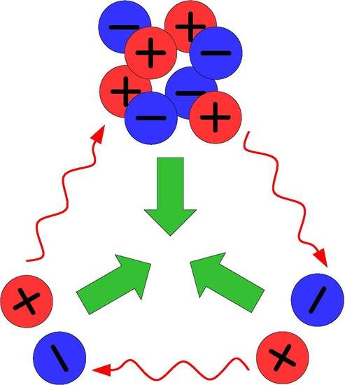
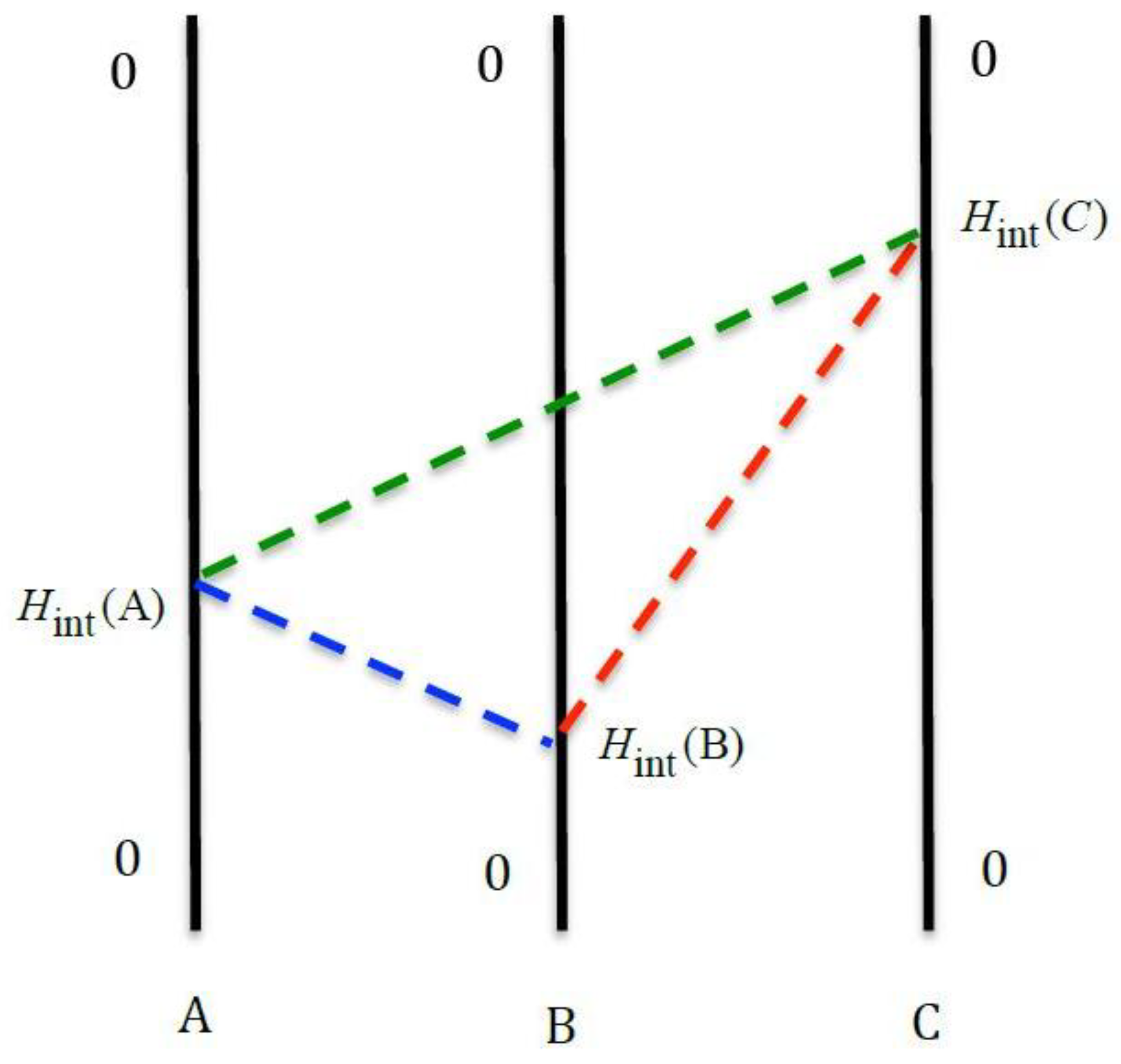
34]. One of the six possible time-ordered sequences containing effective two-photon interaction vertices is shown in
Figure 1. As characteristic of field theories, particles with zero or integer spin—the bosons, mediate interactions between material particles possessing half-integer spin—the fermions. In the case of QED, the electromagnetic force is mediated between electrons by the exchange of virtual photons [
35,
36]. By definition these types of photons are unobservable. They appear from and return to the electromagnetic vacuum with energy and lifetime dictated by Heisenberg’s time-energy uncertainty relation.
For the particular three-body dispersion interactions involving electric octupole coupling to be studied in the remaining, the appropriate effective two-photon interaction Hamiltonians to be used in the diagrammatic perturbation theory calculation are as follows. For a molecule
that is mixed electric dipole-octupole polarisable, coupling to the electromagnetic field occurs via the two-photon interaction operator
where the mixed dipole-octupole polarisability tensor at real wave number is given by
For the same molecule that is pure electric octupole polarisable, the Craig–Power form of the interaction Hamiltonian is
with
defined for molecule C by Equation (3).
At this stage it is convenient to introduce the decomposition of the octupole moment into its irreducible components of weights-1 and -3. Whence
where
and
for the multipole moment defined with respect to the origin.
has three independent components and the transformation properties of a vector, while
has seven independent components. When any two of the Cartesian tensor components are equal, Equation (18) vanishes. Similarly, from the form of the electric octupole coupling to the electric displacement field in either form of interaction Hamiltonian, be it Equation (9) or Equation (13) or Equation (15), the contribution is zero when the suffix of the field is equal to that of any of the gradient operators immediately preceding it. This is because for a neutral entity, the electric displacement field is exclusively transverse in nature outside of the source. It is for the same reason that the trace of the electric quadrupole moment does not contribute to the coupling in the interaction term
It is clear from the partitioning Equation (16) that any mixed polarisability tensor containing an electric octupole moment, or pure electric octupole polarisability Equation (3), may also be separated into contributions that are explicitly dependent upon scalar weight-1 and -3 octupole moment terms. For instance, inserting Equation (16) into the mixed electric dipole-octupole polarisability Equation (14) produces
Analogously, the pure electric octupole polarisability tensor
Equation (3), has octupole weight 1-1, 1-3, 3-1 and 3-3 dependent contributions,
3. DD-DD-DO Energy Shift
The first dispersion potential to be evaluated is the leading correction involving the octupole interaction term, namely that between two electric dipole polarisable molecules A and B, and a third, C, that is mixed electric dipole-octupole polarisable and characterised by Equation (14) or Equation (19). Hence the interaction Hamiltonian for the system of three coupled ground state particles is
with the pure electric dipole Craig–Power coupling Hamiltonian given by Equation (11). Emulating the calculational procedure recently employed in evaluating three-body energy shifts [
14,
15] yields
for an arbitrary triangular configuration of the three particles, with side lengths
a,
b and
c defined earlier. Each polarisability is evaluated at the imaginary frequency. Utilising the definitions of
and
introduced in Equations (5) and (6), allows the energy shift Equation (22) to be written more succinctly as
Both expressions for the energy shift hold for molecules in fixed relative orientation to one another.
To obtain the potential applicable to isotropic molecules, a rotational average of Equation (23) is required. This may be done as separate averages over each particle. For electric dipole polarisable species A and B, the randomly averaged tensor, enclosed in angular brackets, is given by
where the Greek subscripts denote Cartesian tensor components in the molecule-fixed frame of reference, and a factor of 1/3 has been absorbed into the definition of the isotropic polarisability. From expression (19) it is seen that the mixed dipole-octupole polarisability is a sum of weight-1 and -3 octupole moments, and overall is a Cartesian tensor of rank four. An orientational average of such an object is obtained via [
37]
where
is a fourth-rank tensor, and
is given by
From the form of the mixed dipole-octupole coupling Equation (13), it is seen that
vanishes when
j =
k and when
j =
l. Hence the second and third terms within square brackets of Equation (26) do not contribute. Similarly, the mixed dipole-octupole coupling is zero when
and when
so that the second and third terms within each of the three terms written in parentheses do not contribute to the orientational average. Therefore the orientationally averaged mixed electric dipole-octupole polarisability of molecule C appearing in formula (23) is
From relation (16) it is seen that the octupole moment appearing in Equation (27) is composed only of the weight-1 term, with the weight-3 contribution vanishing identically. The superscript “1” serves to label the contributing weight, as in expression (19). On employing relation (24) twice and Equation (27) in Equation (23) yields the energy shift for isotropic molecules
where a factor of 2/15 has been absorbed into the definition of the isotropic mixed dipole-octupole polarisability. Multiplying the geometric tensors using Equations (5) and (6) produces for the dispersion potential.
which applies to a scalene triangle geometry. The circumflex denotes a unit vector. It is interesting to note that each of the eight terms contained within square brackets inside the braces, namely involving direction cosines, appears distinctly in the corresponding expression for the triple dipole dispersion potential (Equation (57) from Ref. [
15]). Because
has transformation properties equivalent to that of an electric dipole, result (29) may be interpreted as a higher-order correction to
Expressions for specific configurations follow straightforwardly from Equation (29). For an equilateral triangle,
a =
b =
c =
R, and
Whence
whose coefficients preceding each power of
uR are identical to corresponding terms appearing in the triple dipole energy shift when the triangle is equilateral (see Equation (48) of Ref. [
14]).
Another noteworthy feature of Equation (29) (and consequently result (30)), is that there is no term independent of
u, leading to no direct near-zone asymptote. This is due to its dependence solely upon the octupole weight-1 term, and the absence of a contribution from the weight-3 term. Nevertheless, by making the following approximations we may arrive at a short-range limiting form for the interaction energy. Retaining the (
uR)
3 term, with
for
uR << 1, and using result (A15) from
Appendix C, we see that Equation (30) results in an
R−8 near-zone limiting dependence on separation distance for an equilateral triangle arrangement:
This compares with an inverse ninth power dependence on R in a true near-zone limit for the triple-dipole potential.
The far-zone limiting form of the interaction energy for an equilateral triangle configuration follows directly from Equation (30) on taking the polarisabilities to be static, corresponding to the zero frequency limit
since in the far-zone
uR >> 1 with
and evaluating the ensuing
u-integral using the standard integral
This leads to the far-zone asymptote
and which exhibits inverse twelfth power separation distance dependence. Note that for this particular three-particle configuration, the force is repulsive.
For a collinear arrangement, in which the mixed dipole-octupole polarisable species C lies mid-way between A and B, 2
a = 2
b =
c =
R, and
and
so that
and
the dispersion energy shift from Equation (29) is
Again the coefficients appearing in the polynomial function are identical to that found for the collinear geometry of three dipole polarisable molecules (Equation (52) of Ref. [
14]), as well as in the weight-1 dependent contribution to the DD-DD-OO dispersion energy shift (see Equation (51) of Ref. [
14]). As for the equilateral triangle case, inverse eighth power law behaviour is found in the near-zone on using result (A15). It is given by
In the radiation zone Equation (34) reduces to
which varies as
R−12. The potentials for the collinear arrangement are positive in sign.
4. DD-DO-DO Dispersion Potential
The next dispersion energy involving octupole moments to be examined is that between an electric dipole polarisable molecule, A, and two mixed electric dipole-octupole polarisable species, B and C. This interaction is of the same order of magnitude as that between two electric dipole polarisable particles, and a third that is pure electric octupole polarisable, and which has previously been published [
14,
15]. The calculation is similar to that outlined in the last section and to other dispersion interactions between three bodies.
Relative to Equation (21) the interaction Hamiltonian is
Summing over the six time-ordered diagrams at third-order of perturbation theory produces the following result for molecules in fixed relative orientation to one another, and which depends on octupole weight-1 and -3 terms:
Orientational averaging using Equations (24) and (27) produces the energy shift expression for isotropic molecules
on absorbing factors of 2/15 into each of the isotropic mixed dipole-octupole polarisabilities, and on making use of the relation
After averaging, the weight-3 octupole moment makes no further contribution to the interaction energy, with only the weight-1 term in play. The product of geometrical tensors produces a result identical in form to that occurring in the octupole weight-1 dependent term of the DD-DD-OO potential given in Equation (54) of Ref. [
15] for a scalene triangle, and to the geometrical part of the triple dipole result, given by Equation (57) of Ref. [
15]. Thus
is another higher-order correction to the
energy shift. Explicitly,
From this last equation, which applies to a scalene triangle arrangement of the three atoms, the dispersion potential for an equilateral triangle geometry is readily found to be
Because there is no
u-independent term, a true near-zone limit does not exist. One may be found by retaining the (
uR)
4 term and using the integral result (A16). This gives a potential with an
R−9 short-range dependence,
At very large separation distances between nuclei, Equation (41) reduces to the far-zone asymptote
displaying
R−14 behaviour, and for which the polarisabilities are static.
For three molecules in a straight line, C lying in the centre,
whose near-zone limiting form exhibits inverse ninth power dependence on using Equation (A16),
In the far-zone Equation (44) gives rise to an asymptotic energy shift
with identical power law dependence to that found for an equilateral triangle geometry, Equation (43). It is interesting to note that the polynomial terms within square brackets of the
u-integrals (41) and (44) are identical to the octupole weight-1 dependent terms occurring in the DD-DD-OO dispersion potential, given by the first integral terms of Equations (47) and (51) of Ref. [
14], respectively, and are therefore necessarily higher-order corrections to the triple dipole potential, as seen by comparing Equations (41) and (44) with Equations (48) and (52) of Ref. [
15].
5. DO-DO-DO Interaction Energy
The next three-body dispersion energy shift involving electric octupole coupling to be studied is that between three mixed electric dipole-octupole polarisable species. The interaction Hamiltonian is the same for each centre, namely
with
given explicitly by Equation (13). Standard calculational procedure leads to the following formula applicable for molecules with locked-in relative configurations,
and is dependent upon octupole weight-1 and -3 contributions. After random orientational averaging there is no dependence on
and the energy shift simplifies to
exhibiting a dependence solely on octupole weight-1 moment as found in each of the previous cases involving mixed dipole-octupole polarisability. A factor of 2/15 has been taken into each of the isotropic mixed polarisability tensors of Equation (49). On multiplying the product of
tensors using Equation (6), the isotropic potential for a scalene triangle is
The eight individual direction cosine terms within braces are identical to those featuring in the triple dipole dispersion potential between three particles in arbitrary geometrical arrangement.
For three atoms or molecules positioned in an equilateral triangle configuration, Equation (50) yields the potential
The coefficients match those computed in Equation (41). Even though there is no
u-independent term, a short-range asymptote may nonetheless be extracted from Equation (51). This is done by substituting Equation (19) for the octupole weight-1 contribution to the mixed dipole-octupole polarisability evaluated at imaginary frequency and making the approximation
so that the product of energy denominators simplifies to
The
u-integral in Equation (51) therefore becomes
which may be evaluated using the integral result (32). This produces 10112
R5/243, yielding a near-zone asymptote
which exhibits
R−10 behaviour.
At very long-range, the limiting form of the energy shift is
with inverse separation distance exponent of sixteen.
For a collinear arrangement, the energy shift is
with identical coefficients to that given in Equation (44). A limiting form of the energy shift which is dominant at short-range may be obtained in an identical manner to that carried out for the equilateral triangle case. Approximating
in the energy denominators of the polarisabilities by
u6, the
u-integral in Equation (55) is evaluated using Equation (32) to give
and a near-zone asymptote
From Equation (55) the far-zone limit of the potential is
which displays an
R−16 dependence.
6. DD-DO-OO Dispersion Potential
The final dispersion interaction energy to be computed involving the electric octupole moment is that between an electric dipole polarisable molecule, A, an electric dipole-octupole polarisable species, B, and a purely electric octupole polarisable particle, C. This potential is of the same order of magnitude as the energy shift considered in the previous section between three mixed electric dipole-octupole polarisable objects. In the present case the interaction Hamiltonian is
with the last contribution given by Equation (15). From third-order perturbation theory and summing the contributions from six time-ordered graphs, the potential for molecules in fixed mutual orientation is
where
is the pure electric octupole polarisability of C, Equation (3).
To obtain the interaction energy for randomly oriented molecules requires an average of
, a sixth-rank Cartesian tensor. Utilising the form of the octupole moment and the nature of its coupling to the transverse electric displacement field, the averaged quantity is [
37]
Contracting tensor indices after multiplying factors from the average over each molecule, and using the relation
and
which follow from Equations (16)–(18), an explicit expression for the energy shift (60) in terms of octupole weights is
It is interesting to note that apart from pre-factors, Equation (62) is identical to the DD-DD-OO dispersion potential given by Equation (53) of Ref. [
15], or if expressed in terms of reducible components of the octupole moment, is equivalent to Equation (46) of Ref. [
15]. This recognition is arrived at on realising that
Thus energy shift formulae for particular geometrical arrangements may be written down immediately from the results presented in Section VI of Ref. [
14].
For the pure electric octupole polarisability having implicit dependence upon octupole weight-1 and -3 dependent terms, where 1/3 is factored into
a factor of 2/15 is absorbed into
but the factor 14/210 is retained explicitly, the dispersion energy for an equilateral triangle configuration is
with coefficients identical to that found in the DD-DD-OO interaction energy. The additional factor
u2/
R2 in each integral term of Equation (63) ensures the potential is entirely retarded, containing no
uR-independent terms, as expected since the mixed dipole-octupole polarisability of
B is independent of the octupole weight-3 term. A form applicable at very short range may be obtained on retaining the
u-independent term in the second integral of Equation (63) and using the integral result (A14). This is found to be
displaying inverse fifteenth power dependence.
With similar definitions for the isotropic polarisabilities, the dispersion potential for collinear geometry is
which also contains no
uR-independent term. Using the result (A14) a short-range limiting form of Equation (65) may be obtained as
which has identical power law behaviour as result Equation (64).
7. Summary
A systematic study has been peformed of dispersion interactions between three molecules when the effects of electric octupole coupling have been accounted for, supplementing a previously published result involving two electric dipole polarisable species, and a third that is pure electric octupole polarisable. This has been carried out using the theory of molecular QED, in which the electromagnetic field is quantised and interactions between non-relativistic microscopic particles take place via the exchange of one or more virtual photons. As in the case of pair dispersion potentials, the transfer of two virtual photons between each interacting pair mediates coupling between three molecules in the ground electronic state, with the radiation field in the vacuum state. To simplify the computations, for instance by considerably reducing the number of time-ordered diagrams that have to be summed over, an extension to higher multipoles of the Craig–Power Hamiltonian operator was adopted instead of the usual interaction Hamiltonian that is linear in the Maxwell field operator. This alternate perturbation operator, which has the form of an effective two-photon coupling operator, enables third-order perturbation theory to be used in the evaluation of the three-body dispersion potential.
Specific energy shifts calculated include that between two electric dipole polarisable molecules and one that is mixed electric dipole-octupole polarisable; one electric dipole polarisable molecule and two mixed dipole-octupole polarisable molecules; and three mixed electric dipole-octupole polarisable molecules. Also computed was the potential between an electric dipole polarisable molecule, an octupole polarisable species, and a mixed dipole-octupole polarisable molecule, which is of the same order as the DO-DO-DO interaction. Important insight into the results obtained was gained by decomposing the octupole moment into its irreducible components of weights-1 and -3. The weight-1 dependent contributions to each of the potentials contained sums of direction cosine terms that preceded polynomial terms in various powers of u, a, b, and c that were identical to that found in the leading non-pairwise additive triple-dipole contribution to the energy shift, with the and previously obtained contributions being viewed as higher-order correction terms to the DD-DD-DD potential.
Interestingly, for isotropic energy shifts involving mixed dipole-octupole polarisable species, the interaction energies are wholly retarded, containing no static terms. Furthermore, the octupole weight-3 term of this tensor vanishes on random orientational averaging, leaving a dependence solely on the weight-1 contribution. Nevertheless, evaluation of the
u-integral for small displacements of the three particles may be used to obtain an energy shift valid in the near-zone. Explicit expressions for dispersion potentials were also given for equilateral triangle and collinear arrangements of the three molecules for each of the multipole moment combinations considered. The hierarchy of emerging power laws in the near-zone can be understood from the fact that the nonretarded DD-DD-DD potential is proportional to
R−9, where each replacement of a dipole with an octupole leads to a factor of the order (
a/
R)
2 << 1, where
a represents the extent of the electronic wave function. On top of this, the absence of true static terms leads to factors (
kR)
m << 1, where
m is zero or a positive integer and
k is the wave number of the radiation exchanged between the molecules. Note that DO-DO and DO-DO-DO interactions are special cases where the exact balance between (
a/
R)
4 and (
a/
R)
6, respectively with (
kR)
4 and (
kR)
6 leads to an additional factor
R−1 arising from a Casimir–Polder type integral. The emerging power laws for pair and three-body interactions are shown in
Table 1.
It is also worth highlighting that the integrals over imaginary wave vector evaluated in the Appendices may be used to calculate the sub-dominant contribution to the near-zone potential between an electric dipole polarisable molecule and an electric octupole polarisable one. This two-body potential has been calculated previously [
29], and is
Strictly speaking there is no contribution to the conventional near-zone limit arising from the first term of Equation (67), that dependent upon octupole weight-1, because there is no
uR-independent term. A short-range asymptote may be arrived at by approximating
in the polarisabilities and using Equation (32) to evaluate the resulting
u-integral, giving
exhibiting a Casimir-like inverse seventh power dependence. The typical near-zone limit, arising from the second term of Equation (67), that dependent upon octupole weight-3, in contrast displays
R−10 behaviour. Again, the unexpected behaviour stems from an additional small factor (
kR)
3, as shown in
Table 1. In this context it is useful to remark that short- and long-range expansions of the Casimir–Polder dispersion potential, as well as all correction terms up to second order in the fine structure constant have been performed from consideration of the orbit-orbit contribution due to the Breit-Pauli Hamiltonian, including relativistic effects [
38,
39], and compared with recent molecular QED calculations [
30].
Finally, it is worth pointing out that the ratio of the limiting forms of the triple dipole dispersion potential for an equilateral triangle configuration to the pair potential is where is the static polarisability, indicating that for small values of this quantity and large separations the triple dipole energy shift is appreciably weaker than the corresponding two-body contribution. Interestingly, taking the electric dipole moment to be where e is the proton charge and a0 is the Bohr radius, and the transition energy to be of the order of one Rydberg, the ratio is unity at distances of around 3a0, with increasing in importance at larger distances.


