Article

A Fuzzy Set-Valued Autoregressive Moving Average Model and Its Applications

1
Department of Statistics, Guangzhou University, No. 230 Waihuanxi Road, Higher Education Mega Center, Guangzhou 510006, China
2
School of Applied Mathematics, Guangdong University of Technology, No. 161 Yinglong Road, Tianhe District, Guangzhou 510520, China
*
Author to whom correspondence should be addressed.
Symmetry 2018, 10(8), 324; https://doi.org/10.3390/sym10080324
Submission received: 23 June 2018 / Revised: 19 July 2018 / Accepted: 2 August 2018 / Published: 7 August 2018

Abstract

:
Autoregressive moving average (ARMA) models are important in many fields and applications, although they are most widely applied in time series analysis. Expanding the ARMA models to the case of various complex data is arguably one of the more challenging problems in time series analysis and mathematical statistics. In this study, we extended the ARMA model to the case of linguistic data that can be modeled by some symmetric fuzzy sets, and where the relations between the linguistic data of the time series can be considered as the ordinary stochastic correlation rather than fuzzy logical relations. Therefore, the concepts of set-valued or interval-valued random variables can be employed, and the notions of Aumann expectation, Fréchet variance, and covariance, as well as standardized process, were used to construct the ARMA model. We firstly determined that the estimators from the least square estimation of the ARMA (1,1) model under some L 2 distance between two sets are weakly consistent. Moreover, the justified linguistic data-valued ARMA model was applied to forecast the linguistic monthly Hang Seng Index (HSI) as an empirical analysis. The obtained results from the empirical analysis indicate that the accuracy of the prediction produced from the proposed model is better than that produced from the classical one-order, two-order, three-order autoregressive (AR(1), AR(2), AR(3)) models, as well as the (1,1)-order autoregressive moving average (ARMA(1,1)) model.

1. Introduction

A time series is a set of observations, each one being recorded at a specified time. Time series analysis has been an important branch of both the stochastic process and mathematical statistics. Various time series can be found in the fields of engineering, science, sociology, and economics. The theory and methods of time series analysis have been extensively developed and achieved great success in the modeling and prediction of time series [1].
There are several famous time series models, such as autoregressive (AR), autoregressive moving average (ARMA), autoregressive integrated moving average (ARIMA), and autoregressive conditional heteroskedasticity (ARCH), which have been proposed for the purpose of future prediction [1]. There is extensive literature on the prediction of the future for some system using these models. For example, Metghalchi et al. proposed testing moving average technical trading rules for the NASDAQ (National Association of Securities Dealers Automated Quatations) composite index. They showed that moving average rules indeed have predictive power and could discern a recurring-price pattern for profitable trading [2]. Li et al. presented an intelligent prediction approach for degradation prognostics of rotating machinery based on an asymmetric penalty sparse decomposition algorithm combined with an autoregressive moving average-recursive least square algorithm (ARMA-RLS) and wavelet neural network [3].
Note that all of the data concerned with the models mentioned above are represented by real numbers or vectors. However, in this big-data era, various complex data have arisen in many fields of sciences and technologies. Among them, the interval-valued data, or more general, the set-valued data, have received great attention in recent years, since they are, in some sense, the extension of incomplete, missing, or censored data. Examples include the interval representing the salary range for a person, the interval representing the range of blood pressure for a person, the range of the weather temperature for a special day in some city, and some data represented by a complex medical image, symmetric color picture, etc. In the system decision-making area, we also face human perception mixed data, such as linguistic data, whose values are not numeric but are words or sentences of some language, some of which can be represented by nearly symmetric fuzzy numbers. We refer to such data as fuzzy data.
Accordingly, in recent years, the stochastic processes with set-valued members have received attention in the literature. Li et al. [4] considered fuzzy set-valued Gaussian processes and Brownian motions, in which the classical Gaussian stochastic process was extended to a case where the process elements are allowed to take values of fuzzy sets, and a new fuzzy Brownian motion was firstly introduced. Bongiorno [5] presented a note on the former Brownian motion, where it was pointed out that the former fuzzy set-valued Brownian motion can be handled by an n-dimensional vector-valued Wiener process, since the expectation of the fuzzy set-valued element is a constant. Furthermore, Wang et al. [6] firstly proposed an interval-valued stationary time series modeling approach, in which an interval-valued p-order autoregressive (AR(p)) model was proposed. Note that, here, they did not considered the stochastic process or time series with linguistic data. These works raise the possibility that some extension of time series modeling [1] to linguistic data (perception mixed data) could be realized under the consideration of ordinary stochastic correlation between the elements of the time series process.
We are aware that interval-valued or linguistic-valued data benefit from having a higher volume of information compared to real number-valued data. For instance, finance and economics are far from being free from imprecision or uncertainty. In the process of reducing some economy-related quantities and magnitudes to numbers and mathematical concepts, we have to deal with a wealth of vague terms (confidence, fear, instability, risk, etc.) which are meaningful for us. For example, a set of stocks with small volatility or countries with high unemployment rates are not crisp descriptions, since the words “small” and “high” are vague in meaning, reflecting a judgment of the observers for the observed objects based on their own perception. Also, the investor’s expected values of the future returns for investments are often given in a linguistic form such as “very optimum”, “around the values of last year’s return”, “may at least cover the cost”, etc. One typical feature of the linguistic data is that the data are characterized with fuzziness, therefore, it is often recommended to employ the fuzzy sets to model the linguistic data. Using a fuzzy set to model linguistic data is meaningful: the fuzzy set is not only easier to apply than words in mathematical modeling, but it also embraces more information with respect to the empirical judgment, as well as the emotional reaction of the human, than that of real numbers.
It has been demonstrated that the extension of time series models to the case of linguistic data (fuzzy data) was developed along two lines—parametric methods and nonparametric methods—in the literature.
When the parametric method is applied, the form of the original time series models is not changed; instead of the original real number-valued data, the linguistic data and their arithmetic operations are used. Such work can be found in Wang [7], in which the authors primarily proposed a special conceptualized p-order autoregressive model AR(p) (where p is a positive integer and p 1 ) with n-dimensional fuzzy data [8] in the way of the set-valued stochastic process, wherein the semi-linear structure of the space of all fuzzy sets, the expectation, variance, and covariance of fuzzy random variables ([9]) are considered for the construction of the model. However, there was no work on the model’s estimation. Wang [10] further noted that former autoregressive models contain some deficiencies, so the model was complemented with an ARMA model and its primary application in financial market forecasting was proposed. Jung et al. [11] also considered a unified approach to asymptotic behavior for parameter estimation for an AR(1) model of a fuzzy number-valued time series, where a brief outline on the modeling of time series with fuzzy number inputs and fuzzy number outputs was given. An illustrative example of the AR(1) model with fuzzy numbers is that of the Dow Jones Industrial Average (DJI) index time series [11]. A significant advantage of the parametric methods is that the original natural relationships between the elements of the time series are maintained and investigated during the modeling.
When the nonparametric method is applied, we not only change the form of the original time series models, but also replace the original data with linguistic data (fuzzy data). There are a number of studies on this topic, which is called a fuzzy time series. For instance, in [12,13], the fuzzy time series were firstly proposed as a series with elements taking the values of linguistic or vaguely described data, and the elements can be linked with each other using fuzzy logical relationships that need to be given subjectively by a human. Various improvements and developments on the above fuzzy logical relationship-based fuzzy time series were given by [14,15,16,17], and others, where more effective forecasting models, such as two-factor high-order fuzzy time series forecasting, deterministic vector long-term forecasting, etc., were proposed. The fuzzy logical relationship-based fuzzy time series modeling methods are largely based on intellectual computing, such as the fuzzy relational equations and approximate reasoning. It should be pointed out that such soft computing methods may optimally capture the fuzzy information involved in the elements of the time series, however, the natural stochastic relationships between the elements of the time series are completely ignored, which may lead not only to a biased prediction for the future when we apply the fuzzy time series models for forecasting, but also to a disdain for investigating the mathematical statistical properties of the time series.
Our main interests are in the parametric methods for modeling the time series with linguistic data mentioned above, where the obtained previous results are reviewed. We are aware that there are several fundamental problems, such as parameter estimation (model estimation), asymptotic properties of the estimators, etc., which remain to be investigated further. For instance, parameter estimation has been carried out only for the AR(1) and ARMA(1,1) models with fuzzy data [10,11], and the asymptotic properties (consistency properties) of the estimators have been obtained only for the AR(1) model with fuzzy data [11]. In this study, based on previous works [7,10,11], we firstly investigated the asymptotic properties of the estimators for a (1,1)-order autoregressive moving average model ARMA(1,1) based on linguistic data (fuzzy data), then used the justified ARMA(1,1) model to forecast the future of the HSI with a simulation analysis.
This article proceeds as follows. In Section 1, the related previous work and some existing problems are discussed. Section 2 introduces the basic concepts of fuzzy sets, arithmetic operations for fuzzy sets, correlation, and independence, as well as expectation and Fréchet variance, and covariance under the L 2 metric δ 2 (proposed by Näther [9]) for fuzzy random variables. In Section 3, the asymptotic properties for a special ARMA model for fuzzy data-valued time series with standardized terms is described, and some extension of the classical results on causality for the ARMA models is presented. In Section 4, an empirical analysis of the proposed models in the linguistic monthly HSI time series modeling and prediction is detailed. In Section 5, we present a conclusion for this article.

2. Preliminaries

2.1. Fuzzy Set on R n

The development of the concept of fuzzy sets was motivated by the need to efficiently process ambiguous information, human natural language, as well as human decision problems. A fuzzy set u ˜ of R n is equivalent to its membership function u ˜ : R n [ 0 , 1 ] , where the number u ˜ ( x ) represents the degree of membership at which x belongs to u ˜ . By F ( R n ) , we denote the collection of all normal, convex, and compact fuzzy sets on R n , i.e., for u ˜ F ( R n ) ,
(1)
There exists x 0 R n such that u ˜ ( x 0 ) = 1 ;
(2)
The α -cut of u ˜ , u ˜ α : = { x R n : u ˜ ( x ) α } , α ( 0 , 1 ] , is a convex and compact set of R n ;
(3)
u ˜ 0 : = c l { x R n : u ˜ ( x ) > 0 } , the support of u ˜ , is compact.
If n = 1 , then the fuzzy set of R is said to be a fuzzy number.
Zadeh’s extension principle [18,19] allows us to apply addition and scalar multiplication on F ( R n ) :
( u ˜ + v ˜ ) ( x ) = sup s + t = x min ( u ˜ ( s ) , v ˜ ( t ) ) , x R n .
( a u ˜ ) ( x ) = u ˜ ( x a ) , a 0 0 , a = 0 a R ,
and for any a , b R , the following holds:
( a b ) u ˜ = a ( b u ˜ ) , a ( u ˜ + v ˜ ) = ( a u ˜ ) + ( a v ˜ ) .
However, it holds only for a b 0 , a , b R
( a + b ) u ˜ = ( a u ˜ ) + ( b u ˜ ) .
It indicates that ( F ( R n ) , + , · ) is not a linear space. With Minkowski’s set operation, it holds that
( u ˜ + v ˜ ) α = u ˜ α + v ˜ α , α ( 0 , 1 ] .
( a u ˜ ) α = a u ˜ α , α ( 0 , 1 ] .
A support function of u ˜ F ( R n ) is defined as
S u ˜ α ( x ) = sup t u ˜ α { x · t } , α ( 0 , 1 ] , 0 , α = 0 . x S n 1 = { x : x = 1 } ,
where · denotes the inner product in the Euclidean space R n . It holds that for u ˜ , v ˜ F ( R n ) and a R ,
S ( u ˜ + v ˜ ) α = S u ˜ α + S v ˜ α .
S ( a u ˜ ) α ( x ) = a S u ˜ α ( x ) , a > 0 ; S ( a u ˜ ) α ( x ) = a S u ˜ α ( x ) , a < 0 .
It holds that
S ( ( a u ˜ ) + ( b v ˜ ) ) α ( x ) = ( a S u ˜ α + b S v ˜ α ) ( x ) , a , b > 0 ( a S u ˜ α + b S v ˜ α ) ( x ) , a , b < 0 .
where α [ 0 , 1 ] . Thus, the semi-linear map S : F ( R n ) L 2 ( S n 1 × [ 0 , 1 ] ) , u ˜ S u ˜ α ( x ) makes us view the fuzzy set u ˜ as a support function equivalently, i.e., the map S embeds F ( R n ) into a cone of functional Hilbert space [20].
Remark 1.
For modeling the fuzzy set-valued time series, the distance between two fuzzy sets needs to be clarified. It is well known that the distance between two real numbers or vectors is an important notion that measures the differences of the two numbers or vectors. Because the fuzzy set is a set, the distance between two fuzzy sets can be a distance between two sets [18]. There are many definitions of distances proposed for fuzzy sets, such as d H , d p , d , ρ p , ρ, etc., defined on F ( R n ) [9,11,18], i.e.,
d H ( A , B ) = max { sup a A inf b B a b , sup b B inf a A a b } ,
where A , B are nonempty subsets of R n ,
a b = i = 1 n ( a i b i ) 2 , ( a 1 , , a n ) , ( b 1 , , b n ) R n .
For u ˜ , v ˜ F ( R n ) ,
d p ( u ˜ , v ˜ ) = 0 1 ( d H ( u ˜ α , v ˜ α ) ) p d α 1 / p , 1 p < .
d ( u ˜ , v ˜ ) = sup α ( 0 , 1 ] { d H ( u ˜ α , v ˜ α ) } ,
ρ p ( u ˜ , v ˜ ) = [ 0 1 ( S n 1 | S u ˜ α ( x ) S v ˜ α ( x ) | p μ ( d x ) ) d α ] 1 / p , 1 p < .
ρ 2 ( u ˜ , v ˜ ) = Z ( S u ˜ α ( x ) S v ˜ α ( x ) ) ( S u ˜ β ( y ) S v ˜ β ( y ) ) d K ( x , α , y , β ) ,
where Z = S n 1 × [ 0 , 1 ] × S n 1 × [ 0 , 1 ] and K is a symmetric positive definite kernel.
Some of sets are much too complicated in regard to the computation of distances [18]. In a practical application, for example, in system decision making, the human’s linguistic judgment or perception of the concerned items can be represented by a fuzzy number, and the distances for such fuzzy numbers should be chosen while considering the ease of computation. In the modeling of time series with fuzzy data, using different metrics, we may obtain different results from the models applied to the problems of interest.
In this work, we used a special distance between u ˜ , v ˜ F ( R n ) , defined by the L 2 metric δ 2 , which is a standard distance with ease of computation, and is widespread in applications using fuzzy data modeling.
δ 2 ( u ˜ , v ˜ ) : = n 0 1 S n 1 | S u ˜ α ( x ) S v ˜ α ( x ) | 2 μ ( d x ) d α 1 / 2 ,
and let
u ˜ , v ˜ : = n 0 1 S n 1 S u ˜ α ( x ) S v ˜ α ( x ) μ ( d x ) d α .
where μ is a normalized Lebesgue measure.
( F ( R n , δ 2 ) is a complete and separable metric space [9,18].
The Hukuhara difference h between two fuzzy sets [21] is defined as follows. Let u ˜ , v ˜ F ( R n ) . If there exists a s ˜ F ( R n ) with u ˜ = v ˜ + s ˜ , then s ˜ is said to be the Hukuhara difference between u ˜ , v ˜ , and it is denoted by s ˜ : = u ˜ h v ˜ . The Hukuhara difference possesses good properties for the operation of the difference between sets. For u ˜ , v ˜ F ( R n ) , it holds that
(1)
u ˜ h u ˜ = { 0 } ;
(2)
( u ˜ + v ˜ ) h v ˜ = u ˜ ;
(3)
u ˜ = v ˜ if and only if u ˜ h v ˜ = v ˜ h u ˜ = { 0 } ;
(4)
S u ˜ α h v ˜ α = S u ˜ α S v ˜ α .
For more properties of the Hukuhara difference, the readers are refereed to Stifanini [22].
Note that u ˜ v ˜ for u ˜ , v ˜ F ( R n ) is a fuzzy arithmetic and is based on Zadeh’s extension principle, which is different from the Hukuhara difference.

2.2. Fuzzy Random Variables (FRVs)

The concept of FRVs was inspired by the attempt to model the randomness and fuzziness that exist in real-life phenomena simultaneously. Typically, there are two kinds of FRVs: the FRVs of Kwakernaak—Kruse and Meyer [23,24] and of Puri-Ralescu [8]. The former is devoted to modeling the human vague perception of a random variable (the original) [24], and the latter is for modeling the completely fuzzy random phenomena of real life [9,23]. Both FRVs are mathematically equivalent to each other when they are valued in F ( R ) , and there are no appropriate distributional models for FRVs [9,23].
Remark 2.
Ref. [8] Let ( Ω , A , P ) be a complete probability space. The mapping X ˜ : Ω F ( R n ) is said to be a fuzzy random variable (FRV) if X ˜ is A B measurable, i.e., for any measurable subset B R n , { ω | X ˜ α ( ω ) B } A , where B is a σ-algebra on R n induced by X ˜ associated with the concerned metric, and X ˜ α ( ω ) : = { x R n | X ˜ ( ω ) α } = [ X ˜ ( ω ) ] α , α [ 0 , 1 ] , ω Ω .
In the following, we assume that the FRV X ˜ is second order under the metric δ 2 , i.e.,
E ( X ˜ 2 ) : = E ( δ 2 2 ( X ˜ , { 0 } ) ) < + .
This condition can ensure the existence of second moments for FRVs [9].
Remark 3.
([8] Aumann expectation) The expectation E X ˜ of an FRV X ˜ is a normal compact fuzzy set of R n with the property that ( E X ˜ ) α = E X ˜ α , α [ 0 , 1 ] , where E X ˜ α is the Aumann expectation of the random set X ˜ α , i.e.,
E X ˜ α = { E η | η ( ω ) X ˜ α ( ω ) , a . e . , η L ( Ω , R ) } ,
where L ( Ω , R ) is the set of all real random variables with the existing expectation defined on Ω, a.e. means almost everywhere.
Let X ˜ be an FRV, then S X ˜ α is a random element and E ( S X ˜ α ) = S E ( X ˜ α ) [9,21] if the Aumann expectation E ( X ˜ α ) exists, α [ 0 , 1 ] ([8,23]).
The concepts of variance and covariance take an important role in stochastic analysis and statistical modeling, and they have been extended to FRVs in several different ways. Based on the extension principle, Kruse and Meyer [24] proposed a kind of fuzzy variance and covariance for FRVs, which seems to be weak from the aspect of keeping the original essence of the variance and covariance. In recent years, it was advocated to propose definitions in which the essence of variance and covariance is kept for FRVs, which means that the variance of an FRV is an accurate measurement of the spread or dispersion of the FRV with its mean, and the covariance or the correlation coefficient of two FRVs must measure their linear interdependence, so they should have no fuzziness [9,25].
Remark 4.
The Fréchet variance of FRV X ˜ w.r.t the distance δ 2 is defined by
V a r ( X ˜ ) : = E ( δ 2 2 ( X ˜ , E ( X ˜ ) ) ) = n 0 1 S n 1 V a r ( S X ˜ α ( x ) ) μ ( d x ) d α .
Remark 5.
The Fréchet covariance of two FRVs X ˜ , Y ˜ w.r.t. the distance δ 2 is defined by
C o v ( X ˜ , Y ˜ ) : = n 0 1 S n 1 C o v ( S X ˜ α ( x ) , S Y ˜ α ( x ) ) μ ( d x ) d α .
Then, the usual classical form
C o v ( X ˜ , Y ˜ ) = E X ˜ , Y ˜ E X ˜ , E Y ˜ ,
V a r ( X ˜ ) = E X ˜ , X ˜ E X ˜ , E X ˜ ,
hold. In the case of n = 1 , since the normalized Lebesgue measure μ ( S 0 ) = 1 , and S 0 = { 1 , 1 } is symmetric, then μ ( 1 ) = μ ( 1 ) = 1 2 , and we have
V a r ( X ˜ ) = 1 2 0 1 ( V a r ( inf X ˜ α ) + V a r ( sup X ˜ α ) ) d α .
C o v ( X ˜ , Y ˜ ) = 1 2 0 1 ( C o v ( inf X ˜ α , inf Y ˜ α ) + C o v ( sup X ˜ α , sup Y ˜ α ) ) d α .
This just coincides with the definitions of variance and covariance for a one-dimensional FRV, proposed by Feng et al. [26], which indicates that Feng’s definitions are a special case of Remark 4 and Remark 5 above.
Lemma 1.
([25]) Let X ˜ and Y ˜ be two FRVs with second order under the metric δ 2 , then
(1) 
V a r ( u ˜ ) = 0 ;
(2) 
V a r ( a X ˜ + b Y ˜ ) = a 2 V a r ( X ˜ ) + b 2 V a r ( Y ˜ ) + 2 a b C o v ( X ˜ , Y ˜ ) , a b 0 , a , b R ;
(3) 
V a r ( a ξ ) = a 2 V a r ξ , a R n , r . v . ξ 0 ;
(4) 
C o v ( ( a X ˜ ) + ( b Y ˜ ) , c Z ˜ ) = a c C o v ( X ˜ , Z ˜ ) + b c C o v ( Y ˜ , Z ˜ ) , a c 0 , b c 0 , a , b , c R ;
(5) 
C o v ( ( a X ˜ ) + u ˜ , b Y ˜ + v ˜ ) = a b C o v ( X ˜ , Y ˜ ) , a b 0 , a , b R , u ˜ , v ˜ F ( R n ) .
Definition 1.
The fraction
R ( X ˜ , Y ˜ ) = C o v ( X ˜ , Y ˜ ) / V a r ( X ˜ ) V a r ( Y ˜ ) ,
a normalized Fréchet covariance, is said to be the Fréchet correlation coefficient of two FRVs. X ˜ , Y ˜ , where V a r ( X ˜ ) > 0 , V a r ( Y ˜ ) > 0 .
The independence of FRVs can follow from the independence of the random elements, which is already defined by [9].
Lemma 2.
([25]) Let X ˜ and Y ˜ be two FRVs with second order under the metric δ 2 , then
(1) 
if X ˜ and Y ˜ are independent, then C o v ( X ˜ , Y ˜ ) = 0 ;
(2) 
| R ( X ˜ , Y ˜ ) | 1 ;
(3) 
R ( X ˜ , Y ˜ ) = 1 if and only if Y ˜ + ( λ E X ˜ ) = E Y ˜ + ( λ X ˜ ) , a.e., R ( X ˜ , Y ˜ ) = 1 if and only if Y ˜ + ( λ X ˜ ) = E Y ˜ + ( λ E X ˜ ) , a.e., where λ = V a r Y ˜ / V a r X ˜ , V a r ( X ˜ ) > 0 , V a r ( Y ˜ ) > 0 .
FRVs X ˜ and Y ˜ are said to be uncorrelated if R ( X ˜ , Y ˜ ) = 0 . If 0 < | R ( X ˜ , Y ˜ ) | < 1 , then there may exist some weak linear dependent relations between X ˜ and Y ˜ .
Now we consider convergence properties of a sequence of FRVs with second order under the metric δ 2 . Note that Feng [26] has already considered some convergence problems under the metric d p for a sequence of one-dimensional FRVs, and under the metric d for a sequence of n-dimensional FRVs. Let { X ˜ n } be a sequence of FRVs with second order, and it is thus X ˜ under the metric δ 2 , δ 2 ( X ˜ n , X ˜ ) is a random variable. Define D 2 ( X ˜ n , X ˜ ) : = [ E ( δ 2 2 ( X ˜ n , X ˜ ) ) ] 1 / 2 . If D 2 ( X ˜ n , X ˜ ) 0 ( n ) , then it is said that the sequence { X ˜ n } of FRVs converges to FRV X ˜ in mean square under metric δ 2 . If δ 2 2 ( X ˜ n , X ˜ ) ) 0 ( n ) in probability, then it is said that the sequence { X ˜ n } of FRVs converges to FRV X ˜ in probability as n . Referring to [26], we the have following theorem.
Theorem 1.
Let { X ˜ n } be a sequence of FRVs with second order, and it is thus X ˜ under the metric δ 2 , then the following conditions are equivalent:
(1) 
D 2 ( X ˜ n , X ˜ ) 0 ( n ) ;
(2) 
{ X ˜ n } is a Cauchy sequence, i.e., lim m , l D 2 ( X ˜ m , X ˜ l ) = 0 ;
(3) 
The series { X ˜ n 2 , n 1 } of random variables is uniformly integrable and δ 2 ( X ˜ n , X ˜ ) ) 0 ( n ) in probability.
Proof. 
(1)⇒ (2): Since D 2 ( X ˜ n , X ˜ ) 0 ( n ) , D 2 ( X ˜ m , X ˜ ) 0 ( m ) , then from the triangle inequality of D 2 , we have
D 2 ( X ˜ n , X ˜ m ) D 2 ( X ˜ n , X ˜ ) + D 2 ( X ˜ , X ˜ m ) 0 ( n , m ) .
(2) ⇒ (3): Since D 2 ( X ˜ n , X ˜ m ) 0 ( m , n ) , which is equivalent to D 2 2 ( X ˜ n , X ˜ m ) 0 ( m , n ) . Using Markov inequality, we have
P ( δ 2 2 ( X ˜ n , X ˜ m ) ϵ ) D 2 2 ( X ˜ n , X ˜ m ) ϵ 0 ( m , n ) ,
for any ϵ > 0 , which means δ 2 2 ( X ˜ n , X ˜ m ) P 0 , as n , m , i.e., { X ˜ n } is a Cauchy sequence of FRVs under the metric δ 2 in probability. From the completeness of the space ( F ( R n ) , δ 2 ) , the sequence { X ˜ n } has a limit valued in F ( R n ) under the metric δ 2 in probability, thus the limit is an FRV, we denote it by X ˜ , and we have δ 2 ( X ˜ n , X ˜ ) P 0 as n . Since each X ˜ n is of second order, it is obvious that X ˜ n 2 is uniformly integrable.
(3) ⇒ (1): Since δ 2 ( X ˜ n , X ˜ ) P 0 as n , and we have
P ( | δ 2 ( X ˜ n , { 0 } ) δ 2 ( { 0 } , X ˜ ) | δ 2 ( X ˜ n , X ˜ ) < ϵ ) 1 ( n ) ,
i.e., X ˜ n P X ˜ as n . By Fatou’s lemma,
E X ˜ 2 lim n inf E X ˜ n 2 sup n E X ˜ n 2 < .
The uniform integrability of { X n ˜ 2 } ( n 1 ) , and the inequality δ 2 2 ( X ˜ n , X ˜ ) 2 ( X ˜ n 2 + X ˜ 2 ) imply that { δ 2 2 ( X ˜ n , X ˜ ) } ( n 1 ) is uniformly integrable. Using the dominated convergence theorem, we have
lim n D 2 2 ( X ˜ n , X ˜ ) = lim n E ( δ 2 2 ( X ˜ n , X ˜ ) ) = 0 .
 ☐
Theorem 2.
Let { X ˜ n } be a sequence of FRVs with second order under the metric δ 2 and sup n E X ˜ n 2 < , { b j } is a non-negative number series satisfying j = 0 b j 2 < , then the infinite semi-linear sum of FRVs j = 0 b j X ˜ j converges in probability under the metric δ 2 .
Proof. 
(1) We prove that j = 0 b j X ˜ j is integrable bounded.
E j = 0 b j X ˜ j = lim r E j = 0 r b j X ˜ j = lim r E δ 2 2 ( j = 0 r b j X ˜ j , { 0 } ) = lim r E n 0 1 S n 1 ( S ( j = 0 r ( b j X ˜ j ) ) α ( x ) S { 0 } ( x ) ) 2 μ ( d x ) d α = lim r E n 0 1 S n 1 ( b 0 S X ˜ 0 α + b 1 S X ˜ 1 α + + b r S X ˜ r α ) 2 μ ( d x ) d α = lim r j = 0 r b j 2 E X ˜ j + lim r i , l = 0 , i l r b i b l E X ˜ i , X ˜ l ( lim r j = 0 r b j 2 ) sup j E X ˜ j 2 + lim r ( i , l = 0 , i l r b i 2 + b l 2 2 ) sup j E X ˜ j 2 < .
(2) We prove that { W n = j = 0 n b j X ˜ j } is a Cauchy sequence under the metric D 2 .
lim r , l D 2 2 ( W r , W l ) = lim r , l E ( δ 2 2 ( W r , W l ) ) = lim r , l E n 0 1 S n 1 ( S ( j = 0 r b j X ˜ j ) α ( x ) S ( j = 0 l b j X ˜ j ) α ( x ) ) 2 μ ( d x ) d α = lim r , l E n 0 1 S n 1 ( j = l + 1 r b j S X ˜ r α ) 2 μ ( d x ) d α lim r , l [ j = l + 1 r b j 2 + i , s = l + 1 , i s r b i 2 + b s 2 2 ] sup j E X ˜ j 2 = 0 sup j E X ˜ j 2 = 0 ,
since lim j b j 2 = 0 . From Theorem 1, we determine that { W n } converges to some FRV W in probability under the metric δ 2 , i.e., j = 0 b j X ˜ j converges in probability under the metric δ 2 . ☐
Remark 6.
In this paper, the expectation, variance, and covariance, as well as the correlation values of FRVs and the convergence of a sequence of FRVs, are defined under the metric δ 2 only. This is obviously a special case from a general FRV point of view. Thus, our concerned autoregressive models for fuzzy data-valued time series are special ones. For obtaining more general models, we may further consider a bit more general metric on F ( R n ) .

3. A Fuzzy Set Valued ARMA Model Based on a Standardized Process

Based on the concepts of the Fréchet covariance and Fréchet linear correlation for the FRVs defined in the former section, we consider some autoregressive models for fuzzy data-valued time series. In a real-world situation, one may perceive such a process as a sequence of investment approximate returns by time. Even the observers timely evaluations on some stock prices may also form such a time series. Note that an example of autoregressive sequence of one-dimensional FRVs and the related correlation function had already been proposed by Feng et al. [26].
Definition 2.
Let { X ˜ t } ( t Z ) be a process of FRVs valued in F ( R n ) with second order under the metric δ 2 . If t denotes the time points, then { X ˜ t } is said to be a fuzzy data valued time series. The Fréchet covariance function C ( l , s ) of the process { X ˜ t } ( t Z ) is defined by C ( l , s ) = C o v ( X ˜ l , X ˜ s ) , l , s Z . The process { X ˜ t } ( t Z ) is said to be wide-sense (weakly) stationary if it holds that C ( l , s ) = C o v ( X ˜ t + l , X ˜ t + s ) , E ( X ˜ t ) , t , l , s Z , are independent of t, where Z is the set of all integers.
Note that for a wide-sense stationary fuzzy data-valued time series, the Fréchet covariance function can be simply denoted by C ( h ) : = C ( h , 0 ) , since C ( l , s ) = C ( l s , 0 ) .
Example 1.
For a process { ξ ˜ t , t Z } of Gaussian FRVs ([27]): ξ ˜ t = E ( ξ ˜ t ) + ξ t , where random vector ξ t N n ( 0 , Σ ) , an n-dimensional Gaussian distribution with zero mean vector, the Fréchet covariance function can be carried out as
C ( t , s ) = C o v ( ξ t , ξ s ) = n S n 1 ( i = 1 n j = 1 n x i x j c o v ( ξ t i , ξ s j ) ) μ ( d x ) ,
where x = ( x 1 , , x n ) S n 1 , ξ t = ( ξ t 1 , , ξ t n ) , ξ s = ( ξ s 1 , , ξ s n ) are real-valued n-dimensional random vectors with multivariate Gaussian distribution N n ( 0 , Σ ) , and c o v ( ξ t i , ξ s j ) is the classical covariance of random variables ξ t i , ξ s j .
It is obvious that a process { ξ ˜ t , t Z } of Gaussian FRVs is mutually uncorrelated in the sense of the Fréchet correlation if and only if the process { ξ t } of the Gaussian random vectors is mutually uncorrelated in the sense of the Fréchet correlation. Note that the Fréchet correlation between two random vectors is different from the conventional concept of correlation of two random vectors in multivariate statistics; the former depends on the Fréchet covariance, whereas the latter depends on the ordinary covariance matrix. Also, in this example, we can determine that the wide-sense stationarity of the process of Gaussian FRVs is equivalent to the wide-sense stationarity of the process of Gaussian random vectors.
In the following, we consider a special error term process, which may help us to propose an applicable ARMA model with fuzzy data in the area of financial data analysis.
Definition 3.
([10]) Let { w ˜ t } ( t Z ) be a process of fuzzy random sets valued in F ( R n ) with second order under the metric δ 2 . { w ˜ t } ( t Z ) is said to be a standardized process of FRVs if it holds that
C o v ( w ˜ t + h , w ˜ t ) = 1 , h = 0 , 0 , h 0 ,
where t , h Z . Obviously, a standardized process { w ˜ t } ( t Z ) of FRVs is wide-sense stationary.
Sometimes, a standardized process of fuzzy random sets { w ˜ t } ( t Z ) can be viewed in the sense of a white noise process, i.e., a fuzzy observation on a conventional white noise process, which means that if ε t is a term of a white noise process { ε t } , t Z , then w ˜ t can be viewed as some fuzzy observation on ε t satisfying the membership value w ˜ t ( ε t ) = 1 . Note that, in general, w ˜ t is not unique, as it depends on the observers’ opinions, and different observers may set different membership functions w ˜ t .
In the one-dimensional case, we present a standardized process of FRVs based on a real-valued white noise process. However, it is difficult to give a standardized process of FRVs in an n-dimensional case ( n 2 ).
Example 2.
Let { ε t } be a white noise process, i.e., E ( ε t ) = 0 , V a r ( ε t ) = 1 , c o v ( ε i , ε j ) = 0 , i j , t , i , j Z . We define a process { w ˜ t } of FRVs as follows,
w ˜ t ( x ) = x ε t + 1 , ε t 1 x ε t , x + ε t + 1 , ε t x ε t + 1 .
It is easy to know that { w ˜ t } is a standardized process of FRVs.
In the following, we always assume that the standardized process of FRVs can be used for modeling the error term process of a time series model with fuzzy data.
Definition 4.
([10]) A process of FRVs { X ˜ t } with second order under the metric δ 2 is said to be a fuzzy set-valued p-order autoregressive (briefly, AR(p) with fuzzy data) process if { X ˜ t } is wide-sense stationary and, for any t Z , it holds that
X ˜ t = θ 1 X ˜ t 1 + θ 2 X ˜ t 2 + + θ p X ˜ t p + w ˜ t ,
where θ i is a real number-valued parameter, { w ˜ t } is a standardized process of FRVs, and p is a natural number.
Definition 5.
([10]) A process of FRVs { X ˜ t } with second order under the metric δ 2 is said to be a fuzzy set-valued ( p , q ) -order autoregressive moving average (briefly, ARMA( p , q ) with fuzzy data) process if { X ˜ t } is wide-sense stationary and, for any t Z , it holds that
X ˜ t = θ 1 X ˜ t 1 + θ 2 X ˜ t 2 + + θ p X ˜ t p + ϕ q w ˜ t q + + ϕ 1 w ˜ t 1 + w ˜ t ,
where θ i , ϕ i are real number-valued parameters, { w ˜ t } is a standardized process of FRVs, and p , q are natural numbers.
An ARMA( p , q ) process { X ˜ t } of FRVs is said to be a causal ARMA( p , q ) process under the metric δ 2 if it has a wide-sense stationary solution almost everywhere, i.e., there exists a positive (or negative) number series { b j } such that j = 0 b j w ˜ t j converges in probability under the metric δ 2 and X ˜ t = j = 0 b j w ˜ t j , a.e., where { w ˜ t } is a standardized process of FRVs.
Example 3.
Let { Y ˜ t } be a wide-sense stationary process of fuzzy random sets with second order, set X ˜ t = Y ˜ t E ( Y ˜ t ) , then, by (5) of Lemma 1, we have C o v ( X ˜ t + h , X ˜ t ) = C o v ( Y ˜ t + h , Y ˜ t ) , thus, { X ˜ t } is wide-sense stationary and with fuzzy zero expectations { 0 ˜ } , where 0 ˜ is independent of t and not unique.
Lemma 3.
([10]) Let { X ˜ t } ( t Z ) be an AR(1) with fuzzy data: X ˜ t = θ X ˜ t 1 + w ˜ t , where { w ˜ t } is a standardized process of FRVs. Then, { X ˜ t } possesses a wide-sense stationary solution X ˜ t = j = 0 θ j w ˜ t j almost everywhere if 0 < θ < 1 , and sup t w ˜ t 2 < .
For the estimation of an AR(1) with fuzzy data based on sample x ˜ 1 , x ˜ 2 , , x ˜ m from the process { X ˜ t } of FRVs with second order, we can determine that
(1)
If the AR(1) model is causal, then an estimator of the parameter θ can be θ ^ = C ^ ( 1 ) C ^ ( 0 ) , where
C ^ ( 1 ) : = 1 m t = 1 m 1 n 0 1 S n 1 ( S ( x ˜ t + 1 ) α ( x ) S x ˜ ¯ α ( x ) ) ( S ( x ˜ t ) α ( x ) S x ˜ ¯ α ( x ) ) μ ( d x ) d α ,
C ^ ( 0 ) : = 1 m t = 1 m n 0 1 S n 1 ( S ( x ˜ t ) α ( x ) S x ˜ ¯ α ( x ) ) 2 μ ( d x ) d α ,
are the sample-based estimators of the Fréchet covariance C ( 1 ) , C ( 0 ) , respectively, and x ˜ ¯ = 1 m t = 1 m x ˜ t .
(2)
If the AR(1) with fuzzy data is not causal, then we may employ the least square method proposed by [20] to estimate the parameter θ .
Now, we consider applying the least square estimation method proposed by [20] under the concerned metric δ 2 to estimate an ARMA(1,1) model X ˜ t = θ 1 X ˜ t 1 + ϕ 1 w ˜ t 1 + w ˜ t , ( t Z ). Assume that we have the observations x ˜ i , i = 0 , , d , on the process, and we generate some terms w ˜ i , i = 0 , , d of a standardized process, where it is assumed that x ˜ 0 = w ˜ 0 = 0 .
The estimation of the model can be carried out by minimizing the function
L ( θ 1 , ϕ 1 ) = i = 1 d δ 2 2 ( x ˜ i , θ 1 x ˜ i 1 + ϕ 1 w ˜ i 1 ) ,
on the set
A : = { θ 1 , ϕ 1 | x ˜ i h ( θ 1 x ˜ i 1 + ϕ 1 w ˜ i 1 ) exists for i = 1 , , d } .
We obtain the least square estimates of the parameters θ 1 > 0 , ϕ 1 > 0 as follows,
θ ^ 1 = i = 1 d x ˜ i , x ˜ i 1 i = 1 d x ˜ i 1 , x ˜ i 1 i = 1 d x ˜ i , x ˜ i 1 i = 1 d x ˜ i 1 , x ˜ i 1 i = 1 d x ˜ i 1 , w ˜ i 1 2 i = 1 d x ˜ i 1 , x ˜ i 1 i = 1 d x ˜ i 1 , w ˜ i 1 2 i = 1 d w ˜ i 1 , w ˜ i 1 i = 1 d x ˜ i 1 , x ˜ i 1 ,
ϕ ^ 1 = i = 1 d x ˜ i , x ˜ i 1 i = 1 d x ˜ i 1 , w ˜ i 1 i = 1 d x ˜ i 1 , x ˜ i 1 i = 1 d x ˜ i , w ˜ i 1 i = 1 d x ˜ i 1 , w ˜ i 1 2 i = 1 d w ˜ i 1 , w ˜ i 1 i = 1 d x ˜ i 1 , x ˜ i 1 ,
and θ ^ 1 > 0 , ϕ ^ 1 > 0 , otherwise, the estimators θ ^ 1 , ϕ ^ 1 are not a suitable solution.
If the parameters θ 1 < 0 , ϕ 1 < 0 , then their least square estimators can be carried out by replacing x ˜ i 1 , w ˜ i 1 with x ˜ i 1 , w ˜ i 1 , respectively, in the above formula of θ ^ 1 , ϕ ^ 1 .
The asymptotic properties of the least square estimators for ARMA( 1 , 1 ) with fuzzy data can be given as follows.
Theorem 3.
Let { X ˜ t } be an ARMA(1,1) process with fuzzy data X ˜ t = θ 1 X ˜ t 1 + ϕ 1 w ˜ t 1 + w ˜ t , ( θ 1 > 0 , ϕ 1 > 0 ) and the least square estimators θ ^ 1 , ϕ ^ 1 shown in (42),(43) exist on A : = { θ 1 , ϕ 1 | x ˜ i h ( θ 1 x ˜ i 1 + ϕ 1 w ˜ i 1 ) exists for i = 1 , , d } under the selected distance δ 2 based on a sample { x ˜ i , i = 0 , , d } . If E ( w ˜ i ) 0 , i = 0 , , d , and w ˜ i , w ˜ j and w ˜ s , w ˜ l are uncorrelated for ( i , j ) ( s , l ) , i , j , s , l { 1 , 2 , , d } , and V a r ( w ˜ i , w ˜ j ) = 0 , 0 < θ 1 < 1 , ϕ 1 > 0 , then the least square estimators θ ^ 1 , ϕ ^ 1 are weakly consistent. In a special case of ϕ 1 = 1 , θ ^ 1 , ϕ ^ 1 are consistent.
Proof. 
From (42), the definition of · , · , and the equality x ˜ t = θ 1 x ˜ t 1 + ϕ 1 w ˜ t 1 + w ˜ t , we have
θ ^ 1 θ 1 = ( 1 θ 1 ) ( i = 1 d x ˜ i 1 , w ˜ i 1 ) 2 i = 1 d w ˜ i 1 , w ˜ i 1 ( ϕ 1 i = 1 d x ˜ i 1 , w ˜ i 1 + i = 1 d x ˜ i 1 , w ˜ i ) i = 1 d x ˜ i 1 , w ˜ i 1 2 i = 1 d w ˜ i 1 , w ˜ i 1 i = 1 d x ˜ i 1 , x ˜ i 1 .
Replacing x ˜ t 1 with x ˜ t 1 = θ 1 x ˜ t 2 + ϕ 1 w ˜ t 2 + w ˜ t 1 , then x ˜ t = θ 1 2 x ˜ t 2 + θ 1 ϕ 1 w ˜ t 2 + ( θ 1 + ϕ 1 ) w ˜ t 1 + w ˜ t . Iterating the above equality, it holds that:
x ˜ t = θ 1 t x ˜ 0 + θ 1 t 1 ϕ 1 w ˜ 0 + ( θ 1 t 1 + θ 1 t 2 ϕ 1 ) w ˜ 1 + ( θ 1 t 2 + θ 1 t 3 ϕ 1 ) w ˜ 2 + ( θ 1 t 3 + θ 1 t 4 ϕ 1 ) w ˜ 3 + + ( θ 1 t k + θ 1 t k 1 ϕ 1 ) w ˜ k + + ( θ 1 + ϕ 1 ) w ˜ t 1 + w ˜ t .
By the assumption and Definition 3 and (34), we have E w ˜ i , w ˜ j = E w ˜ i , E w ˜ j = 0 , ( i j ) , E w ˜ i , w ˜ i = 1 , and
E w ˜ i , x ˜ j = 0 , i > j , 1 , i = j , θ 1 j i + θ 1 j i 1 ϕ 1 , i < j .
E x ˜ i , x ˜ i = 1 + ( θ 1 + ϕ 1 ) 2 + ( θ 1 2 + θ 1 ϕ 1 ) 2 + ( θ 1 3 + θ 1 2 ϕ 1 ) 2 + + ( θ 1 i 1 + θ 1 i 2 ϕ 1 ) 2 = 1 θ 1 2 i + 2 ϕ 1 θ 1 ( 1 θ 1 2 ( i 1 ) ) + ϕ 1 2 ( 1 θ 1 2 ( i 1 ) ) 1 θ 1 2 .
Also, we have
E w ˜ i , w ˜ j w ˜ s , w ˜ l = 1 , i = j and s = l , 0 , otherwise .
E w ˜ i , w ˜ j 2 = 1 , i = j , 0 , i j .
Set the numerator and the denominator of (44) as follows,
S 1 : = ( 1 θ 1 ) ( i = 1 d x ˜ i 1 , w ˜ i 1 ) 2 i = 1 d w ˜ i 1 , w ˜ i 1 ( ϕ 1 i = 1 d x ˜ i 1 , w ˜ i 1 + i = 1 d x ˜ i 1 , w ˜ i ) .
D 1 : = i = 1 d x ˜ i 1 , w ˜ i 1 2 i = 1 d w ˜ i 1 , w ˜ i 1 i = 1 d x ˜ i 1 , x ˜ i 1 .
From (45), we have E x ˜ i , w ˜ i 2 = E w ˜ i , w ˜ i 2 = 1 , and E ( i = 1 d x ˜ i 1 , w ˜ i 1 ) 2 = ( d 1 ) 2 ,
E i = 1 d w ˜ i 1 , w ˜ i 1 ( ϕ 1 i = 1 d x ˜ i 1 , w ˜ i 1 + i = 1 d x ˜ i 1 , w ˜ i ) = ϕ 1 ( d 1 ) 2 .
Thus, we have E ( S 1 ) = ( 1 ϕ 1 ) ( d 1 ) 2 . It can also be determined that E ( S 1 2 ) is bounded, since E ( x ˜ i , w ˜ j 2 ) E ( x ˜ i 2 w ˜ j 2 ) , E ( x ˜ i , w ˜ j x ˜ s , w ˜ l ) E ( x ˜ i w ˜ j x ˜ s w ˜ l ) . By the assumption and Chebyshev’s inequality, it holds that S 1 ( d 1 ) 2 p 1 ϕ 1 . After computation, it can also be determined that
E ( D 1 ) = d 1 ( 1 θ 1 2 ) 2 [ ( d 2 ) ( θ 1 2 θ 1 4 ) θ 1 4 ( 1 θ 1 2 ( d 1 ) ) + 2 ( d 2 ) θ 1 ϕ 1 ( 1 θ 1 2 ) 2 θ 1 3 ϕ 1 ( 1 θ 1 2 ( d 2 ) ) + ( d 2 ) ϕ 1 2 ( 1 θ 1 2 ) ϕ 1 2 θ 1 2 ( 1 θ 1 2 ( d 2 ) ) ] ,
and E ( D 1 2 ) is bounded, by the assumption and Chebyshev’s inequality, it holds that
D 1 ( d 1 ) 2 p 1 ( 1 θ 1 2 ) 2 [ θ 1 4 θ 1 2 + 2 θ 1 ϕ 1 ( θ 1 2 1 ) + ϕ 1 2 ( θ 1 2 1 ) ] .
Thus,
S 1 D 1 = S 1 / ( d 1 ) 2 D 1 / ( d 1 ) 2 p 1 ϕ 1 1 ( 1 θ 1 2 ) 2 [ θ 1 4 θ 1 2 + 2 θ 1 ϕ 1 ( θ 1 2 1 ) + ϕ 1 2 ( θ 1 2 1 ) ] ,
i.e., θ 1 ^ θ 1 p 1 ϕ 1 1 ( 1 θ 1 2 ) 2 [ θ 1 4 θ 1 2 + 2 θ 1 ϕ 1 ( θ 1 2 1 ) + ϕ 1 2 ( θ 1 2 1 ) ] .
Obviously, θ 1 ^ θ 1 p 0 when ϕ 1 = 1 , i.e., θ ^ 1 is consistent.
Set the numerator and the denominator of (43) as follows,
S 2 : = i = 1 d x ˜ i , x ˜ i 1 i = 1 d x ˜ i 1 , w ˜ i 1 i = 1 d x ˜ i 1 , x ˜ i 1 i = 1 d x ˜ i , w ˜ i 1 ,
D 2 : = i = 1 d x ˜ i 1 , w ˜ i 1 2 i = 1 d w ˜ i 1 , w ˜ i 1 i = 1 d x ˜ i 1 , x ˜ i 1 ,
Then, we have E ( D 2 ) = E ( D 1 ) , and E ( D 2 2 ) is bounded, by the assumption and Chebyshev’s inequality, it holds that
D 2 ( d 1 ) 2 p 1 ( 1 θ 1 2 ) 2 [ θ 1 4 θ 1 2 + 2 θ 1 ϕ 1 ( θ 1 2 1 ) + ϕ 1 2 ( θ 1 2 1 ) ] .
Also, we have E ( S 2 ) = ( d 1 ) 2 ( 1 ϕ 1 ) ϕ 1 ( d 1 ) ( 1 θ 1 2 ) 2 [ ( d 2 ) ( θ 1 2 θ 1 4 ) θ 1 4 ( 1 θ 1 2 ( d 1 ) ) + 2 ( d 2 ) θ 1 ϕ 1 ( 1 θ 1 2 ) 2 θ 1 3 ϕ 1 ( 1 θ 1 2 ( d 2 ) ) + ( d 2 ) ϕ 1 2 ( 1 θ 1 2 ) ϕ 1 2 θ 1 2 ( 1 θ 1 2 ( d 2 ) ) ] and E ( S 2 2 ) is bounded, by the assumption and Chebyshev’s inequality, it holds that
S 2 ( d 1 ) 2 p 1 ϕ 1 + ϕ 1 ( 1 θ 1 2 ) 2 [ θ 1 4 θ 1 2 + 2 θ 1 ϕ 1 ( θ 1 2 1 ) + ϕ 1 2 ( θ 1 2 1 ) ] ,
Thus,
S 2 D 2 = S 2 / ( d 1 ) 2 D 2 / ( d 1 ) 2 p 1 ϕ 1 1 ( 1 θ 1 2 ) 2 [ θ 1 4 θ 1 2 + 2 θ 1 ϕ 1 ( θ 1 2 1 ) + ϕ 1 2 ( θ 1 2 1 ) ] + ϕ 1 ,
i.e., ϕ 1 ^ ϕ 1 p 1 ϕ 1 1 ( 1 θ 1 2 ) 2 [ θ 1 4 θ 1 2 + 2 θ 1 ϕ 1 ( θ 1 2 1 ) + ϕ 1 2 ( θ 1 2 1 ) ] . ☐
Remark 7.
(1) The proposed AR, ARMA model for the processes of FRVs is an extension of the autoregressive sequence model proposed by Feng et al. [26].
(2) In the proposed models, the so-called standardized process of FRVs plays an important role, as the causality of the AR(p) and ARMA( p , q ) with fuzzy data are defined, and we only present an example of the standardized process in the one-dimensional case. This standardized process is a special error term process only.
(3) In the general case, without the restriction of the second order for the FRVs, the processes of the FRVs may not be posed for the standardized processes, and, at most, we may set an AR(p) with fuzzy data as
X ˜ t = θ 1 X ˜ t 1 + θ 2 X ˜ t 2 + + θ p X ˜ t p + B ˜ t ,
where { B ˜ t } is only an unexplained remainder process of the plus operation among the successive p + 1 elements in process { X ˜ t } , and it may be no longer standardized, t Z . This general case is a hard open problem.
(4) The considered metric δ 2 can also be extended to a general metric, like ρ, given in the literature [9,25].

4. An Empirical Analysis of the ARMA( p , q ) Models with Fuzzy Data

In this section, we consider an empirical analysis for the proposed ARMA model with fuzzy data so as to demonstrate the goodness of the model. To this end, we use the following procedure: Step (1) investigate and collect the data from a practical time series related to the concerned problem; Step (2) generate the perception mixed fuzzy data based on the real data; Step (3) select and estimate the model based on the obtained fuzzy data; Step (4) give the results of prediction using the estimated model; Step (5) compare the model with other available models.
It is well known that the financial market is a complex, non-stationary, noisy, chaotic, and dynamic system. The main reason is the fact that a huge amount of information is reflected in the financial market. The main factors include the economic condition, political situation, traders’ expectations and emotions, catastrophes, and other unexpected events. Stock market data have to be considered in the framework of uncertainties. Therefore, predictions of stock market prices and their directions with high accuracy are quite difficult.
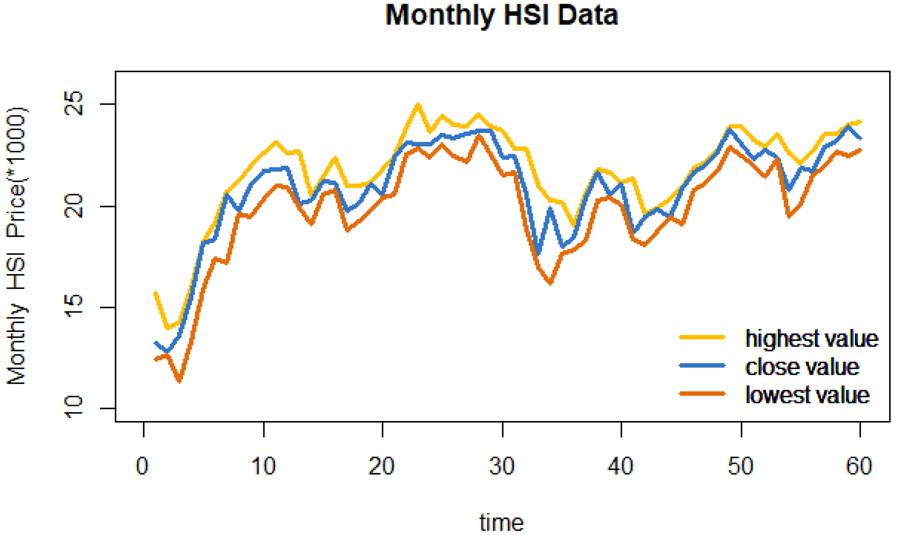
We consider the problem of predicting the trends of monthly HSI by means of the ARMA models for linguistic data, and here the linguistic data are the perception mixed HSI data.
Step 1
Consider the observations in three time series of close value, low value, and high value of the monthly HSI in the time period from January 2009 to December 2013, as shown in Figure 1, where, for simplicity, the employed data are the original data divided by 1000. Generally speaking, the observations can be simply expressed as a finite number series. For instance, since there are a total of 60 months in the time period from January 2009 to December 2013, we may assume that the three finite series { m i } , { a i } , { b i } , i = 1 , , 60 denote the observations in the three time series for close value, low value, and high value in the time period from January 2009 to December 2013, respectively; here, i is a serial number.
Step 2
Note that each monthly data implies very complex information about the random variation of the market, the psychological responses, and judgment-based behaviors of the market participators in one month-long period. In order to gain more informative predictions of the HSI trends, it is suggested to use the three data—the close value, low value, and high value—simultaneously in an appropriate way, in which the evaluator’s perception ought to be mixed, and the perception has to be vague, since the background information hidden behind the three data is so complicated that there is no way to make the perception clear. Though some predictions can be made through the ordinary time series models using a single close value or average value during the time period, the predicted judgment could be much more biased, as the data used here lack completeness of information. Therefore, we view the three values (close value, low value, high value) of each monthly data integrally as linguistic data, i.e., perception mixed financial data, and model it with a simple triangular (or symmetric ) fuzzy number ( L R -fuzzy number [9]) defined on the interval [low value, high value] of the fluctuation. As mentioned above, by m i , a i , b i we denote the close value, low value, and high value of the ith observation of the monthly HSI, respectively, and, according to the expression of an L R -fuzzy number [9], the three data form a simple L R -fuzzy number
( m i , m i a i , b i m i ) L R ,
where m i , m i a i , b i m i denote the core, the left spread, and the right spread of the L R fuzzy number ( m i , m i a i , b i m i ) L R , respectively, ( i = 1 , , 60 ), and L , R denote the shape functions of the L R -fuzzy number. For simplicity, the shape functions are often taken as L ( x ) = R ( x ) = max { 0 , 1 x } . According to this procedure, the linguistic monthly data of HSI from January 2009 to December 2013 can be determined, and they are shown in Table 1. (Note that the serial numbers i = 61 , 62 , represent Jan. 2014, Feb. 2014, ⋯, respectively.)
Step 3
For L R -fuzzy data u ˜ = ( m , l , r ) L R , whose α -cut is u ˜ α = [ m l L ( 1 ) ( α ) , m + r R ( 1 ) ( α ) ] , α [ 0 , 1 ] , where L ( 1 ) ( α ) = R ( 1 ) ( α ) = 1 α for the above L ( x ) , R ( x ) , we have the support function of u ˜ α as
S u ˜ α ( x ) = m + ( 1 α ) r , x = 1 , m ( 1 α ) l , x = 1 .
and the sample-based Fréchet covariance for linguistic monthly HSI in Table 1 can be computed using
C o v ( u ˜ j + h , u ˜ j ) = 1 60 j = 1 60 h [ 0 1 ( S ( u ˜ j + h ) α ( 1 ) S u ˜ ¯ α ( 1 ) ) ( S ( u ˜ j ) α ( 1 ) S u ˜ ¯ α ( 1 ) ) d α + 0 1 ( S ( u ˜ j + h ) α ( 1 ) S u ˜ ¯ α ( 1 ) ) ( S ( u ˜ j ) α ( 1 ) S u ˜ ¯ α ( 1 ) ) d α ] = 1 60 j = 1 60 h [ 0 1 m j + h + ( 1 α ) r j + h m ¯ ( 1 α ) r ¯ ( m j + ( 1 α ) r j m ¯ ( 1 α ) r ¯ ) d α + 0 1 ( 1 α ) l j + h m j + h ( 1 α ) l ¯ + m ¯ ( 1 α ) l j m j ( 1 α ) l ¯ + m ¯ d α ] .
The wide-sense stationarity of the considered linguistic monthly HSI time series may be obtained approximately from the stationarity of both series
0 1 S ( u ˜ j ) α ( 1 ) d α = m j + r j 2 and 0 1 S ( u ˜ j ) α ( 1 ) d α = l j 2 m j , j = 1 , , 60 .
The magnitude of the sample autocorrelation functions of the latter two series decay geometrically to zero, and the sample partial autocorrelation functions are negligible for lags greater than 1. Thus, we may fit an ARMA(1,1) with fuzzy data for the linguistic monthly HSI time series, because usually an ARMA is better than an AR, though the AR(1) with fuzzy data can also be employed here [11]. For estimating the model, according to Definition 3, a standardized process of FRVs { w ˜ t } is generated, as shown in Table 2, based on a generated white noise process { ε t } .
For the estimation of the parameters, here we assume that this standardized process { w ˜ t } basically satisfies the condition of Theorem 3. Applying Equations (42) and (43) of the least square estimators for the ARMA(1,1) model with fuzzy data in Section 3 to the data from Table 1 and Table 2 (the case of d = 60 , n = 1 ), we obtain the estimated ARMA(1,1) of the concerned linguistic monthly HSI with Matlab as
X ˜ i = 0.992 X ˜ i 1 + 0.104 w ˜ i 1 + w ˜ i .
Step 4
For the simplicity of computation and comparison, we only consider the prediction for the former 10 months in 2014. A predicted linguistic monthly HSI for the 10 months from January 2014 to October 2014 (the serial numbers i = 61 , 62 , 63 , 64 , 65 , 66 , 67 , 68 , 69 , 70 . ) are obtained using the prediction formula X ˜ ^ i = 0.992 X ˜ i 1 + 0.104 w ˜ i 1 ; both the real linguistic monthly HSI and the obtained predicted linguistic monthly HSI for the 10 months are shown in Table 3.
Table 3, in fact, also gives a direct comparison between the real and the predicted linguistic monthly HSI. The comparison indicates that the obtained forecasting model is quite reasonable in capturing the complex uncertain and imprecise information, since the linguistic forecasted data provide more information than the crisp data, so the decision makers could consider the best and worst possible situations. On the other hand, the accuracy of forecasting using this model could be improved by adjusting the terms of the standardized process.
Step 5
Note that the predicted linguistic monthly HSI in Table 3, in fact, gives the predictions of the close value series, low value series, and high value series of the monthly HSI simultaneously. Thus, the comparisons of the real close values with the predicted close values, the real low values with the predicted low values, and the real high values with the predicted high values can be done. For instance, the comparison of the close values shown in Table 4 indicates that the predictions for values numbered 62, 65, 66, 67, 68, 70 in the list are with absolute errors less than 0.632, relative errors less than 2.74%, and the predictions for the remainder values have absolute errors within the interval ( 0.632 , 1.239 ) , and relative errors within the interval ( 2.74 % , 5.62 % ) . Similarly, the comparisons regarding the low values and high values, respectively, of the monthly HSI can also be carried out.
Remark 8.
The study of the fuzzy set-valued time series modeling is just in its infancy. There are only two estimated fuzzy set-valued models like AR(1) and ARMA(1,1) [10,11] that can be considered for model comparison under special conditions. However, it is obvious here that the fuzzy set-valued ARMA(1,1) model is better than the fuzzy set-valued AR(1) model for the forecast of the linguistic monthly HSI data. On the other hand, it may not be appropriate to compare the fuzzy set-valued time series models with the classical time series models straightforwardly, since the types of data treated by the two kinds of time series are different.
In a special case, we may compare the predicted close values obtained by the proposed fuzzy set-valued ARMA(1,1) model above with the predicted close values obtained by the ordinary AR(1) or AR(2) or AR(3) or AR(1,1) models through a comparison of their prediction absolute errors and relative errors (note that using time series technology, it can be verified that the ordinary AR(1) or AR(2) or AR(3) or AR(1,1) models can be appropriately applied for the prediction of the concerned time series of close values). The comparison results of AR(1) or AR(2) or AR(3) or AR(1,1) with the real close values are shown in Table 5, Table 6, Table 7 and Table 8, respectively. Finally, a comparison result of the prediction errors from the fuzzy ARMA(1,1) with the prediction errors from AR(1), AR(2), AR(3), and AR(1,1) for the case of close values of the monthly HSI are shown in Table 9, which indicates that, on average, the prediction accuracy of our proposed model is better than that of the other four ordinary time series models, since the average absolute error 0.691 of fuzzy ARMA(1,1) is less than the average absolute errors 1.182, 1.194, 1.487, 1.191 of AR(1), AR(2), AR(3), ARMA(1,1), respectively. Further, the average relative error 3.03% of fuzzy ARMA(1,1) is less than the average relative errors 5.03%, 5.08%, 6.29%, 5.07% of AR(1), AR(2), AR(3), ARMA(1,1), respectively. Also, the error data shown in Table 9 indicate that for the months numbered 61,63,66,67,68,70, both the absolute errors and the relative errors of fuzzy ARMA(1,1) are less than those of AR(1), AR(2), AR(3), ARMA(1,1), thus, the prediction accuracy of our proposed model is better than that of the other four ordinary time series models. For the month numbered 62, the absolute errors and the relative errors of fuzzy ARMA(1,1) are slightly larger than those of AR(1), AR(2), AR(3), ARMA(1,1), but the differences for the absolute errors and relative errors are not more than 0.086 and 0.34%, respectively. Thus, the prediction accuracy of our proposed model is almost the same as that of the other four ordinary time series models. For the month numbered 64, the absolute errors and the relative errors of fuzzy ARMA(1,1) are larger than those of AR(1), AR(2), AR(3), ARMA(1,1), but the differences for the absolute errors and relative errors are not more than 0.454 and 2.059%, respectively, thus, the prediction accuracy of our proposed model is not better than that of the other four ordinary time series models. For the month numbered 65,the absolute errors and the relative errors of fuzzy ARMA(1,1) are slightly larger than those of AR(1), AR(2), ARMA(1,1); the differences for the absolute errors and relative errors are not more than 0.048 and 0.207%, respectively, but the absolute errors and the relative errors of fuzzy ARMA(1,1) are less than those of AR(3), thus, the prediction accuracy of our proposed model is not better than that of the other three ordinary time series models AR(1), AR(2), ARMA(1,1), but it is better than that of AR(3). For the month numbered 69, the absolute errors and the relative errors of fuzzy ARMA(1,1) are slightly larger than those of AR(1), AR(2), ARMA(1,1); the differences for the absolute errors and relative errors are not more than 0.547 and 2.39%, respectively, but the absolute errors and the relative errors of fuzzy ARMA(1,1) are less than those of AR(3), thus, the prediction accuracy of our proposed model is not better than that of the other three ordinary time series models AR(1), AR(2), ARMA(1,1), but it is better than that of AR(3).
Similarly, the same comparison can be done for the high values and low values of the monthly HSI.

5. Conclusions

The ARMA models are important in many fields and applications, although they are most widely applied in time series analysis. In this big-data era, various complex data, such as interval-valued data, linguistic data, etc., have arisen. Theoretically, it is meaningful and valuable to extend the statistical regression models and time series models to such complex data, and such research has recently received much attention. In this paper, we extended the ARMA model to the case of linguistic data that can be modeled by some symmetric fuzzy sets. We firstly determined that the estimators from the least square estimation of the ARMA(1,1) model under some L 2 distance between two sets are weakly consistent. To verify the effectiveness of the proposed linguistic-valued ARMA models, we applied them to forecast the linguistic monthly Hang Seng Index (HSI) with an empirical analysis, and detailed comparisons of the models with other classical AR(1), AR(2), AR(3) models, as well as the ARMA(1,1) model, are given. Furthermore, we present theoretical proofs for some conclusions on the convergence properties of the sequence of the FRVs mentioned in this paper [10].
It should be pointed out that the semi-linear structure of the space of all fuzzy data make us consider all the parameters to be positive or negative, and the estimation of parameters for a high-order (the order is larger than 3) AR and ARMA models with fuzzy data becomes much more complicated. The theory of time series with FRVs (fuzzy set-valued data) needs to be further studied. In relation to the present paper, we expect to further investigate several problems: (1) The asymptotic properties of the least square estimators for the general model ARMA( p , q ); (2) Improving the accuracy level of the forecasting using the fuzzy set-valued ARMA(1,1), AR(1) models.

Author Contributions

D.W. wrote and revised the paper. L.Z. handled the data, figure and computation with software. All authors read and approved the final version of the manuscript.

Funding

This research was funded by (The National Natural Science Foundation of China) grant number (11271096).

Acknowledgments

This research is supported by the NNSF of China under grant number No. 11271096. The author very appreciate the financial aids. The authors also thank the editors and anonymous referees who commented on this manuscript.

Conflicts of Interest

The authors declare no conflict of interest.

References

  1. Brockwell, P.J.; Davis, R.A. Time Series: Theory and Methods, 2nd ed.; Springer-Verlag: New York, NY, USA, 1991. [Google Scholar]
  2. Metghalchi, M.; Chang, Y.H.; Du, J. Technical trading rules for NASDAQ composite intex. Int. Res. J. Finance Econ. 2011, 73, 109–121. [Google Scholar]
  3. Li, Q.; Liang, S.Y. Intelligent Prognostics of Degradation Trajectories for Rotating Machinery Based on Asymmetric Penalty Sparse Decomposition Model. Symmetry 2018, 10, 214. [Google Scholar] [CrossRef]
  4. Li, S.; Guan, L. Fuzzy set-valued Gaussian processes and Brownian motions. Inf. Sci. 2007, 177, 3251–3259. [Google Scholar] [CrossRef]
  5. Bongiorno, E.G. A note on fuzzy set-valued Brownian motion. Stat. Prob. Lett. 2012, 82, 827–832. [Google Scholar] [CrossRef] [Green Version]
  6. Wang, X.; Zhang, Z.; Li, S. Set-valued and interval-valued stationary time series. J. Multivar. Anal. 2016, 145, 208–223. [Google Scholar] [CrossRef]
  7. Wang, D. An autoregressive model with fuzzy random variables. In Soft Methods for Handling Variability and Imprecision, Advances in Soft Computing 48; Dubois, D., Ed.; Springer-Verlag: Berlin, Germany, 2008; pp. 401–448. [Google Scholar]
  8. Puri, M.; Ralescu, D. Fuzzy Random Variables. J. Math. Anal. Appl. 1986, 114, 409–422. [Google Scholar] [CrossRef]
  9. Näther, W. On random fuzzy variables of second order and their application to linear statistical inference with fuzzy data. Metrika 2000, 51, 201–221. [Google Scholar] [CrossRef]
  10. Wang, D. A note on autoregressive models with fuzzy random variables. J. Stat. Theor. Prac. 2018, 12, 356–369. [Google Scholar] [CrossRef]
  11. Jung, H.Y.; Lee, W.J.; Yoon, J.H. A unified approach to asymptotic behaviors for the autoregressive model with fuzzy data. Inf. Sci. 2014, 257, 127–137. [Google Scholar] [CrossRef]
  12. Song, Q.; Chissom, B.S. Fuzzy time series and its models. Fuzzy Sets Syst. 1993, 54, 269–277. [Google Scholar] [CrossRef]
  13. Song, Q.; Chissom, B.S. Forecasting enrollments with fuzzy time series—Part I. Fuzzy Sets Syst. 1993, 54, 1–9. [Google Scholar] [CrossRef]
  14. Guan, S.; Zhao, A. A Two-Factor Autoregressive Moving Average Model Based on Fuzzy Fluctuation Logical Relationships. Symmetry 2017, 9, 207. [Google Scholar] [CrossRef]
  15. Chen, S.M. Forecasting enrollments based on fuzzy time series. Fuzzy Sets Syst. 1996, 81, 311–319. [Google Scholar] [CrossRef]
  16. Li, S.-T.; Kuo, S.-C.; Cheng, Y.-C.; Chen, C.-C. Deterministic vector long-term forecasting for fuzzy time series. Fuzzy Sets Syst. 2010, 161, 1852–1870. [Google Scholar] [CrossRef]
  17. Lee, L.W.; Wang, L.H.; Chen, S.M.; Leu, Y.H. Handling forecasting problem based on two-factors high-order fuzzy time series. IEEE Trans. Fuzzy Syst. 2006, 14, 468–477. [Google Scholar] [CrossRef]
  18. Diamond, P.; Kloeden, P. Metric Spaces of Fuzzy Sets; World Scientific: London, UK, 1994. [Google Scholar]
  19. Zadeh, L.A. The concept of a linguistic variable and its application to approximate reasoning-I. Inf. Sci. 1975, 8, 199–249. [Google Scholar] [CrossRef]
  20. Wang, D.; Shi, M. Estimation of a simple multivariate linear model for fuzzy random sets. In Strengthening Links Between Data Analysis and Soft Computing, Advances in Intelligent Systems and Computing 315; Grzegorzewski, P., Ed.; Springer: New York, NY, USA, 2015; pp. 201–208. [Google Scholar]
  21. Wünsche, A.; Näther, W. Least-square fuzzy regression with fuzzy random variables. Fuzzy Sets Syst. 2002, 130, 43–50. [Google Scholar] [CrossRef]
  22. Stefanini, L. A generalization of Hukuhara difference and division for interval and fuzzy arithmetic. Fuzzy Sets Syst. 2010, 161, 1564–1584. [Google Scholar] [CrossRef]
  23. Krätschmer, V. Probability theory in fuzzy sample space. Metrika 2004, 60, 67–189. [Google Scholar] [CrossRef]
  24. Kruse, R.; Meyer, K. Statistics with Vague Data; Springer Science & Business Media: New York, NY, USA, 1987. [Google Scholar]
  25. Wang, D.; Yasuda, M. Some asymptotic properties of point estimation with n-dimensional fuzzy data. Statistics 2004, 38, 167–181. [Google Scholar] [CrossRef]
  26. Feng, Y.H.; Hu, L.J.; Shu, H.S. The variance and covariance of fuzzy random variables and their applications. Fuzzy Sets Syst. 2001, 120, 487–497. [Google Scholar] [CrossRef]
  27. Puri, M.D.; Ralescu, D. The concept of normality of fuzzy random variables. Ann. Proba. 1985, 13, 1373–1379. [Google Scholar] [CrossRef]
Figure 1. The curves of the close value, low value, and high value for monthly Hang Seng Index (HSI). (https://www.hsi.com.hk/eng).
Symmetry 10 00324 g001
Table 1. Linguistic monthly HSI from January 2009 to December 2013 ( ( m , l , r ) : = ( m , l , r ) L R ).
YearMonthDataYearMonthData
20091(13.278, 0.839, 2.485)20121(20.39, 2.07, 0.2)
2(12.811, 0.177, 1.165)2(21.68, 1.411, 0.08)
3(13.576, 2.23, 0.681)3(20.555, 0.181, 1.086)
4(15.52, 2.188, 0.457)4(21.094, 1.059, 0.011)
5(18.171, 2.316, 0.056)5(18.629, 0.251, 2.756)
6(18.378, 1.002, 0.784)6(19.441, 1.385, 0.138)
7(20.573, 3.387, 0.139)7(19.796, 1.086, 0.073)
8(19.724, 0.132, 1.473)8(19.482, 0.032, 0.818)
9(20.956, 1.529, 0.975)9(20.84, 1.764, 0.055)
10(21.752, 1.447, 0.868)10(21.641, 0.874, 0.206)
11(21.821, 0.819, 1.278)11(22.03, 0.932, 0.119)
12(21.872, 0.939, 0.722)12(22.657, 0.969, 0.061)
20101(20.121, 0.205, 2.551)20131(23.729, 0.869, 0.187)
2(20.268, 1.185, 0.172)2(23.02, 0.575, 0.924)
3(21.239, 0.664, 0.212)3(22.299, 0.323, 0.963)
4(21.108, 0.345, 1.281)4(22.737, 1.314, 0.125)
5(19.765, 0.974, 1.247)5(22.392, 0.102, 1.12)
6(20.128, 0.917, 0.829)6(20.803, 1.377, 1.761)
7(21.029, 1.251, 0.09)7(21.883, 1.764, 0.187)
8(20.536. 0.164, 1.27)8(21.731, 0.266, 0.964)
9(22.358, 1.828, 0.081)9(22.859, 0.911, 0.695)
10(23.096, 0.592, 0.77)10(23.206, 0.566, 0.328)
11(23.007, 0.224, 1.981)11(23.881, 1.418, 0.133)
12(23.035, 0.653, 0.577)12(23.306, 0.593, 0.805)
20111(23.447, 0.39, 0.987)
2(23.338, 0.892, 0.644)
3(23.527, 1.404, 0.407)
4(23.72, 0.252, 0.748)
5(23.684, 1.165, 0.24)
6(22.398, 0.89, 1.308)
7(22.44, 0.829, 0.395)
8(20.534, 1.666, 2.274)
9(17.592, 0.593, 3.382)
10(19.864, 3.694, 0.409)
11(17.989, 0.376, 2.184)
12(18.434, 0.613, 0.6)
Table 2. The former 60 elements of a standardized process of fuzzy random variables (FRVs).
i w ˜ i i w ˜ i i w ˜ i
1(1.80482, 0.01, 0.01)21(1.30572, 0.001, 0.0001)41(−1.3595, 0.00008, 0.0001)
2(−0.07992, 0.007, 0.008)22(1.42513, 0.0003, 0.0002)42(−2.33134, 0.001, 0.00012)
3(0.39658, 0.01, 0.002)23(−0.4158, 0.0002, 0.0001)43(−0.40969, 0.00012, 0.0006)
4(−1.08332, 0.0015, 0.001)24(1.61438, 0.0003, 0.001)44(0.6542, 0.0003, 0.0001)
5(2.23829, 0.01, 0.001)25(−1.05773, 0.001, 0.00002)45(0.39926, 0.00003, 0.00001)
6(−0.62423, 0.001, 0.001)26(−0.94833, 0.0001, 0.001)46(−0.46931, 0.00002, 0.0006 )
7(0.51366, 0.002, 0.001)27(0.95365, 0.0003, 0.001)47(0.86633, 0.0003, 0.00001)
8(−0.08661, 0.0002, 0.0013)28(0.39198, 0.0002, 0.0001)48(−0.92372, 0.0002, 0.00008)
9(−0.59418, 0.0002, 0.001)29(−0.07614, 0.00102, 0.0001)49(1.27746, 0.0001, 0.00002)
10(0.03189, 0.002, 0.0012)30(1.22056, 0.0017, 0.00018)50(−1.4526, 0.0001, 0.001)
11(−0.7378, 0.00021, 0.0013)31(−0.63084, 0.00016,0.00018)51(0.34892, 0.0002, 0.0001)
12(−0.25014, 0.01, 0.0003)32(−0.63576, 0.001, 0.0001)52(−0.05535, 0.00012, 0.0001)
13(0.685, 0.0013, 0.00011)33(−0.34, 0.001, 0.00008)53(−1.228, 0.0008, 0.0001)
14(−0.80416, 0.0013, 0.0003)34(0.07628, 0.0001, 0.0002)54(0.14502, 0.0001, 0.00006)
15(−0.74428, 0.0011, 0.0003)35(0.95536, 0.000016, 0.00011)55(−0.8395, 0.0001, 0.00032)
16(−0.7955, 0.0002, 0.0001)36(−1.2167, 0.0001, 0.00011)56(−0.09626, 0.00009, 0.0006)
17(0.34071, 0.001, 0.0001)37(1.18449, 0.0006, 0.0003)57(−0.85758, 0.0001, 0.00002)
18(−0.30051, 0.001, 0.00017)38(−0.34369, 0.0002, 0.0003)58(0.76497, 0.00002, 0.001)
19(−1.34985, 0.00031, 0.0005)39(1.09024, 0.0001, 0.00006)59(0.04501, 0.000016, 0.00001)
20(0.4327, 0.0001, 0.0002)40(−0.13531, 0.0002, 0.0001)60(1.92838, 0.00008, 0.0002)
Table 3. The real linguistic monthly HSI and the predicted linguistic monthly HSI.
iReal Linguistic Monthly HSIPredicted Linguistic Monthly HSI
61(22.035, 0.289, 1.434)(23.274, 0.381, 0.236)
62(22.836, 1.639, 0.15)(23.662, 0.313, 0.368)
63(22.151, 1.014, 0.688)(23.182, 0.121, 0.502)
64(22.133, 0.037, 1.091)(23.311, 0.248, 0.308)
65(23.081, 1.401, 0.128)(23.402, 0.313, 0.470)
66(23.19, 0.388, 0.207)(23.431, 0.402, 0.487)
67(24.756, 1.63, 0.156)(24.217, 0.418, 0.501)
68(24.742, 0.552, 0.492)(24.406, 0.419, 0.537)
69(22.932, 0.077, 2.43)(24.100, 0.428, 0.558)
70(23.998, 1.433, 0.048)(23.579, 0.432, 0.563)
Table 4. A comparison of the predicted close values obtained by the fuzzy set-valued autoregressive moving average (ARMA)(1,1) with the real close values in the monthly HSI.
iReal Close ValuesPredicted Close ValuesAbsolute ErrorRelative Error
6122.03523.2741.2395.62%
6222.83623.4620.6262.74%
6322.15123.1821.0314.654%
6422.13323.2101.0774.869%
6523.08123.3020.2210.957%
6623.19023.4130.2230.95%
6724.75624.2170.5392.17%
6824.74224.4060.3361.356%
6922.93224.1001.1685.09%
7023.99823.5790.4191.746%
Table 5. A comparison of the predicted close values obtained by the classical AR(1) with the real close values in the monthly HSI.
iReal Close ValuesPredicted Close ValuesAbsolute ErrorRelative Error
6122.03523.6631.6287.38%
6222.83623.4580.6222.723%
6322.15123.2641.1135.02%
6422.13323.0810.9484.283%
6523.08122.9080.1730.75%
6623.1922.7460.4441.91%
6724.75622.5922.1648.74%
6824.74222.4482.2949.27%
6922.93222.3110.6212.7%
7023.99822.1831.8157.56%
Table 6. A comparison of the predicted close values obtained by the classical AR(2) with the real close value in the monthly HSI.
iReal Close ValuesPredicted Close ValuesAbsolute ErrorRelative Error
6122.03523.6581.6237.36%
6222.83623.4470.6112.67%
6322.15123.2471.0964.94%
6422.13323.060.9274.19%
6523.08122.8830.1980.86%
6623.1922.7170.4732.04%
6724.75622.5612.1958.87%
6824.74222.4142.3289.41%
6922.93222.2750.6572.86%
7023.99822.1451.8357.65%
Table 7. A comparison of the predicted close values obtained by the classical AR(3) with the real close value in the monthly HSI.
iReal Close ValuesPredicted Close ValuesAbsolute ErrorRelative Error
6122.03523.6881.6537.5%
6222.83623.3820.5462.4%
6322.15123.0650.9144.1%
6422.13322.7560.6232.81%
6523.08122.4730.6082.63%
6623.1922.2190.9714.19%
6724.75621.9932.76311.16%
6824.74221.7942.94811.91%
6922.93221.621.3125.72%
7023.99821.4672.53110.5%
Table 8. A comparison of the predicted close values obtained by the classical ARMA(1,1) with the real close value in the monthly HSI.
iReal Close ValuesPredicted Close ValuesAbsolute ErrorRelative Error
6122.03523.661.6257.37%
6222.83623.450.6142.69%
6322.15123.2521.1014.97%
6422.13323.0660.9234.21%
6523.08122.890.1910.83%
6623.1922.7250.4652%
6724.75622.572.1868.83%
6824.74222.4232.3199.37%
6922.93222.2860.6462.82%
7023.99822.1561.8427.68%
Table 9. A comparison of the proposed fuzzy set valued ARMA(1,1) with the classical AR(1), AR(2), AR(3), and ARMA(1,1) in the prediction errors for the close value of the monthly HSI.
ifuzzy ARMA(1,1)AR(1)AR(2)AR(3)ARMA(1,1)
abs.err., rel.err.abs.err., rel.err.abs.err., rel.err.abs.err., rel.err.abs.err., rel.err.
611.239, 5.62%1.628, 7.38%1.623, 7.36%1.653, 7.5%1.625, 7.37%
620.626, 2.74%0.622, 2.723%0.611, 2.67%0.546, 2.4%0.614, 2.69%
631.031, 4.654%1.113, 5.02%1.096, 4.94%0.914, 4.1%1.101, 4.97%
641.077, 4.869%0.948, 4.283%0.927, 4.19%0.623, 2.81%0.923, 4.21%
650.221, 0.957%0.173, 0.75%0.198, 0.86%0.608, 2.63%0.191, 0.83%
660.223, 0.95%0.444, 1.91%0.473, 2.04%0.971, 4.19%0.465, 2%
670.539, 2.17%2.164, 8.74%2.195, 8.87%2.763, 11.16%2.186, 8.83%
680.336, 1.356%2.294, 9.27%2.328, 9.41%2.948, 11.91%2.319, 9.37%
691.168, 5.09%0.621, 2.7%0.657, 2.86%1.312, 5.72%0.646, 2.82%
700.449, 1.746%1.815, 7.56%1.835, 7.65%2.531, 10.5%1.842, 7.68%
ave.0.691, 3.02%1.182, 5.033%1.194, 5.085%1.487, 6.292%1.191, 5.076%
(abs. = absolute, rel. = relative, err. = error, ave. = average).

