Intelligent Image Processing System for Detection and Segmentation of Regions of Interest in Retinal Images

Abstract

The automatic detection, segmentation, localization, and evaluation of the optic disc, macula, exudates, and hemorrhages are very important for diagnosing retinal diseases. One of the difficulties in detecting such regions of interest (RoIs) with computer vision is their symmetries, e.g., between the optic disc and exudates and also between exudates and hemorrhages. This paper proposes an original, intelligent, and high-performing image processing system for the simultaneous detection and segmentation of retinal RoIs. The basic principles of the method are image decomposition in small boxes and local texture analysis. The processing flow contains three phases: preprocessing, learning, and operating. As a first novelty, we propose proper feature selection based on statistical analysis in confusion matrices for different feature types (extracted from a co-occurrence matrix, fractal type, and local binary patterns). Mainly, the selected features are chosen to differentiate between similar RoIs. The second novelty consists of local classifier fusion. To this end, the local classifiers associated with features are grouped in global classifiers corresponding to the RoIs. The local classifiers are based on minimum distances to the representatives of classes and the global classifiers are based on confidence intervals, weights, and a voting scheme. A deep convolutional neural network, based on supervised learning, for blood vessel segmentation is proposed in order to improve the RoI detection performance. Finally, the experimental results on real images from different databases demonstrate the rightness of our methodologies and algorithms.

1. Introduction

Eye disorders can lead partial or even total loss of vision, significantly affecting life quality [1]. In order to ensure timely medical intervention and treatment, their early detection relies on the analysis of retinal components such as optic disc (OD), macula (MA), blood vessels (BVs), exudates (EXs), and hemorrhages (HEs). Only intelligent processing of a retinal image can provide real measures of these specific ophthalmological zones. Adding complex image processing to dedicated neural networks and efficient descriptors and classifiers, the system for determining the RoIs in retinal images can be considered as an effective support for decision-making in early disease diagnosis. The system’s input is the retinal image and the output is the degree of retinal RoI damage. Automatic detection based on specific imaging devices and real-time image processing can be used for the early-stage decision of an ophthalmologist. Computer-aided diagnosis in an intelligent system also has the advantages of computational power, speed, and continuous development. Many different approaches for retinal RoI identification and evaluation are found in the literature. However, accurate and simultaneous detection, localization, and evaluation of OD, MA, BV, EX, and HE is a difficult task for such a system. The general difficulty for simultaneous detection of retinal RoIs is the symmetries between them, like between OD and EX (color and, sometimes, segmented shapes) and between EX and HE (segmented shapes). It must have intelligent algorithms for image processing and interpretation and sufficient computational power. Usually, it must exclude the similarities (symmetries) and point out the differences.

The first RoI, the OD, is the easiest to detect, due to its shape, colors, size, and structure. Therefore, many papers are related to its detection and localization [2,3,4,5,6,7,8,9,10,11,12,13,14]. For example, the maximum number of decisions from a set of detectors can be used to detect the center of the OD [7]. By selecting some textural features and image decomposition in overlapping boxes, OD detection becomes more simple and efficient [4]. Taking into account the density of large blood vessels in the OD region, the authors in [6,8] proposed fast and accurate methods for OD detection. Considering that the OD has the highest radial symmetry, a methodology based on the radial symmetry detector and separation of vascular information is used in [14] for OD localization. Sometimes, the OD and EX are similar in color, intensity, and shape. In pathological images, a large EX can be similar to the OD. To overcome this inconvenience, an automatic OD detection is proposed in [13], based on the symmetry axis of blood vessel distribution in this region. Some authors remove the OD before the detection and localization of EXs. To this end, the authors in [15] proposed a methodology to differentiate EXs from ODs by considering the features on different color components. The optic disc is identified as a region where the majority of pixels have a great difference on R and G channels. Next, a thresholding method is applied in order to extract the exudates from the obtained binary image. Some features like mean intensity, entropy, uniformity, standard deviation, and smoothness are computed for obtaining an improved accuracy. The mentioned characteristics have different values for EXs and ODs; so, EXs can be identified by removing the areas that do not have matching values of the previous characteristics. For the optic disc detection, in [16], an algorithm based on the 2D Gaussian filter and blood vessel segmentation was implemented. Also for OD detection Pereira et al. [17] applied a modern algorithm based on ant colony optimization and anisotropic diffusion. More recently, the authors in [18] proposed a supervised model for OD abnormality detection for different datasets, taking into account a deep learning approach from global retinal images. The results show a good accuracy and indicate potential applications. Automatic image analysis methods aiming to detect and segment MA and fovea are currently based on support vector machine classification [19], hierarchical image decomposition [20,21], statistical segmentation methods [22], deep learning [23], and pixel intensity characteristics [24]. The authors in [7] presented a method which combines different OD and MA classifiers to benefit from their strong points (high accuracy and low computation time). With the purpose of detection of macular degeneration, Veras et al. [25] proposed some algorithms to localize and segment the MA. Sekhar et al. [26] addresses blood vessels localization, segmentation, and their spatial relations in order to detect the optic disc and macula. Based on pixel intensity (low), the authors in [27] also proposed the MA detection technique. They also proposed an algorithm for the OD diameter estimation. Akram et al. [28] presented a system based on artificial intelligence for evaluation of macular edema to support the ophthalmologists in early detection of the disease. They used a comprehensive characteristics group and a Gaussian-mixture-model-based classifier for accurate detection of MA. Chaudhry et al. [29] detect macula from an autofluorescence imaging device in connection with OD position. This automatic positioning is based on a top-down approach using vascular tree segmentation and skeletonization. In [30] the authors proposed a method to detect and localize the macula center using two steps: first, the context - based information is aggregated with a statistical type model in order to obtain the approximate localization of the macula; second, the aggregation of seeded mode tracking is used for final localization of the macula center.

Over time, many methods and approaches have been used for the detection of EXs (e.g., thresholding methods considering the green channel [31,32,33]). As a consequence that the illumination conditions are different, image preprocessing algorithms for correction are necessary. Kaur and Mittal [34] proposed an algorithm for EX detection which first identifies and rejects the healthy areas based on their characteristics and second segments the EXs from the remaining regions using a region growing method. Bu et al. [35] presented a hierarchical procedure for EX detection in eye fundus images to solve some difficulties such as the recognition of similar-colored objects (e.g. cotton wool spots, optic disc, and the normal macular reflection). Using an artificial intelligence method, an automated identification of EXs is obtained in [36]. After an initial primary processing phase, an image segmentation based on fuzzy clustering is used and a dataset of regions of interest is obtained. For each area, characteristics such as size, color, edge, and texture are extracted. The authors proposed a deep neural network, based on the extracted characteristics for the detection of areas containing EXs. The images are firstly filtered by applying a fuzzy clustering technique. Furthermore, the method in [37] localizes and evaluates the exudates, taking into account different image processing techniques, morphological filters, and image features.

The approaches for HE identification commonly used can also be grouped into different categories such as thresholding, segmentation, mathematical morphology, classification, clustering, neural network, etc. For example, Seoud et al. [38] described and validated a method for the identification of micro-aneurysms and HEs in retinal images, which can be used in the diagnosis and grading of diabetic retinopathy. Their contribution is a set of dynamic shape features which show the evolution of shapes under a processed image and allow differentiation between lesions and blood vessels. The method was tested against six image datasets, both public and private. A splat-based feature classification algorithm with applications to large, irregular HE detection in retinal images was proposed in [39].

For detection and segmentation of retinal RoIs, different classifiers were used: model-based (template matching), minimum distance between vector features, voting scheme, and, recently, neural network (NN). Garcia et al. [40] proposed an algorithm for computer - based identification of the lesions due to the diabetic retinopathy. The algorithm is integrated into a system in order to support the ophthalmologist decision in the detection and monitoring of the disease. The authors analyze the performance of three different NN classifiers in automated detection of lesions or exudates: support vector machine, radial basis function, and multilayer perceptron. By applying different criteria and testing on 67 images, they conclude that the multilayer NN classifier based on image criterion has the best results. This research was extended in [41], where new criteria and classifiers (e.g., logistic regression) were tested against those in the previous paper. Now, the relationship between the extracted set of characteristics and the class of objects is highlighted. Again, the multilayer perceptron performed the best out of the selected methods, but only by a small margin in comparison with logistic regression. Moreover, in [42] a new neural network supervised approach for blood vessel detection was proposed. The proposed algorithm uses an NN arhitecture for pixel classification and creates a vector of moment-invariants-based and gray-level features for pixel representation. The performance of the algorithm was tested on STARE [43] and DRIVE [44] datasets, with better performance than other existing solutions. The authors in [45] used CNNs (Convolutional NNs) to detect hemorrhages. They tried to simplify and speed it up by heuristically classifying samples of the training phase.

The authors in [46] presented a methodology and their implementation which is based on a voting procedure with the aim of raising the decision accuracy. They proposed the technique of majority voting and probability approach to evaluate the correctness of decision. The important goal of the work consisted in solving detection problems in image processing algorithms which are geometrically constrained. For example, the algorithm performance was tested with good accuracy for OD identification on the MESSIDOR dataset [47]. In order to increase the performances of classifications, the voting scheme and NN approaches were combined in [48]. In this case, two connected NNs were considered: one for feature selection and the other for classification, based on local detectors. Finally, a voting scheme with different weights for local classifiers was used, taking into account the results from associated confusion matrices.

In order to increase the efficiency of the classifiers, primary processing of retinal images is necessary. Therefore, Nayak et al. [49,50] presented algorithms for identification and monitoring glaucoma and diabetic retinopathy, using primary processing l (histogram equalization, filtering, and morphological operations). For a particular disease, specific characteristics are established. Based on these features, an artificial NN classifier identifies the presence of a particular disease and its evolution. The authors in [51] introduce an algorithm based on morphological operations for the identification of micro-aneurysms and HEs in retinal images. The image is firstly primary processed and then, important regions of interest such as OD, blood vessels, and fovea are successively removed from the retinal image. Only the HEs and micro-aneurysms remain. The obtained results are similar to those of other papers as sensitivity and specificity. The method for computer aided detection of the diabetic retinopathy, developed in [52], consists of the following phases: image enhancement by local histogram equalization, Gabor filters, SVM (support vector machine) classifier, HE detection, fovea localization, and diabetic retinopathy identification. The algorithms were implemented and tested on free database HRF [53] with acceptable sensitivity and specificity. The authors in [54] presented a method and algorithms for successive detection of important RoIs in retinal images using an artificial neural network (ANN) and k-means clustering. The ANN was simulated on a common PC and it created time-consuming difficulties for real implementation. The application was developed only for the MESSIDOR database.

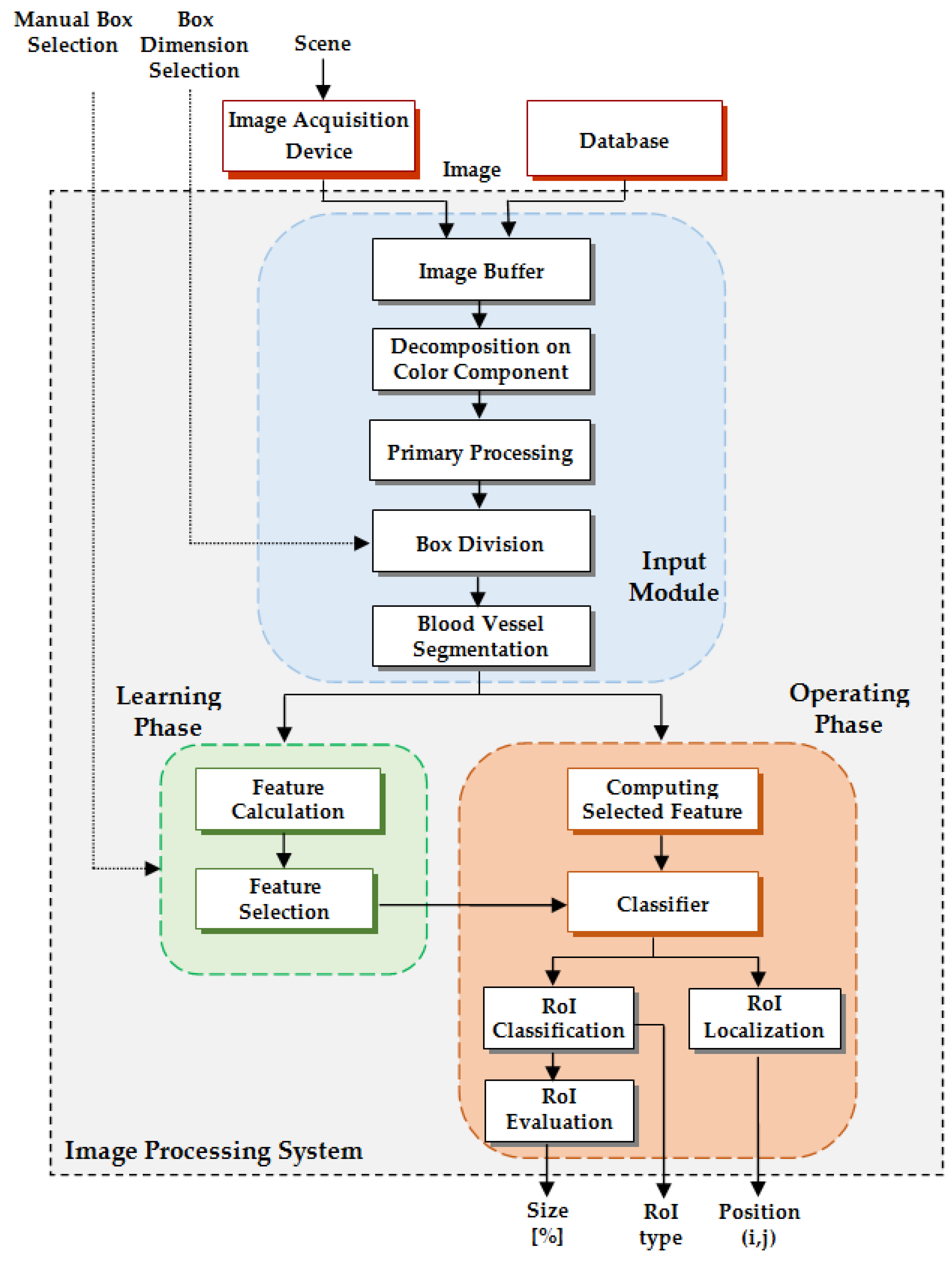
As a technical novelty, this paper proposes an Intelligent System for diagnosis and evaluation of regions of interest from Retinal Images (ISRI), with multiple functions: F1, OD detection; F2, MA detection; F3, EX detection and size evaluation; and F4, HE detection and size evaluation. All of these four functions are addressed. Two main contributions of the authors can be mentioned: (a) proper feature selection based on statistical analysis in confusion matrices for different feature type, and (b) the weight-based fusion of the local classifiers (associated with features) into global classifiers (corresponding to the RoIs). The paper is organized as follows: In Section 2, the methodology and algorithms for primary processing of retinal images with the goal of RoI detection, segmentation, and size estimation are described and implemented. In Section 3 the experimental results obtained using images from two databases (STARE and MESSIDOR) are reported and analyzed. Finally, the discussions and conclusions are presented in Section 4 and Section 5, respectively.

2. Materials and Methods

2.1. ISRI Architecture

We propose an algorithm and software implementation for the identification and evaluation of four RoIs from retinal images: OD, MA, EX, and HE. It can be considered as an intelligent image processing system and diagnosis support for eye diseases. The basic methodology for determination of the mentioned RoIs is texture analysis in small patches (boxes). ISRI has three inputs (retinal image, I; box dimension setting, BDS; and manual box selection, MBS—the last two only for the learning phase) and three outputs (RoI type, RoI; RoI localization, L(i,j); and size estimation of RoI, S [%]). The ISRI concept is shown in Figure 1. As can be seen, it has two phases: a Learning Phase (LP), considered as a calibration one, and an Operating Phase (OP), considered as a measuring one. Also, ISRI has an Input Module (IM) for image preprocessing which is active in both phases.

The IM contains five blocks configured in a pipeline structure: Image Buffer (IB), Decomposition on Color Components (DCC), Primary Processing (PP), Box Division (BD), and Blood Vessel Segmentation (BVS). The retinal image may come from an Image Acquisition Device (IAD) or from an Image Database (DB) and it is stored in the IB to then be processed. First, it is decomposed in color components of RGB and HSV (Hue—Saturation—Value) spaces by DCC. This image is processed by the PP block to improve the representation using the CLAHE algorithm (Contrast-Limited Adaptive Histogram Equalization [38]). Images to be analyzed are further decomposed in boxes by the BD block with the aid of two algorithms: the sliding box algorithm (Figure 2a) and the nonoverlapping box algorithm (Figure 2b). The box dimension is manually selected (Box Dimension Selection, BDS) depending of the image resolution, the algorithm for division, and the type of RoI. The last operation in this initial image processing phase is the blood vessel segmentation by the BVS block.

The LP contains two successive steps: Step 1, calculating the values of a set of features for the regions of interest (Feature Calculation module, FC); and Step 2, selecting effective features for class representation (Feature Selection module, FS). For the LP, manually selected boxes are used (Manual Box Selection, MBS). There are also two successive steps in the OP: Step 1, calculating the values of the selected features corresponding to different RoIs for the boxes extracted from the input image (Computing Selected Features module, CSF); and Step 2, assigning the class label to the RoI (Classifier module, C). RoI_C selects the box type (OD, MA, EX, HE) as a consequence of the RoI classifiers’ decisions. The size evaluation of the detected RoI is done by segmentation and “1”s counting in the RoI_E block. RoI localization is done by the RoI_L block as the position of the upper corner (i,j) of the investigated box.

In order to calibrate and test the system, two well-known public databases were used: STARE [43] and MESSIDOR [47]. They contain both healthy subjects and pathological cases with abnormalities. The STARE database consists of 400 retinal images captured by a TopCon TRV-50 fundus camera. It also contains two sets of manual segmentations obtained by two ophthalmologists used as references. The MESSIDOR database contains three sets of eye fundus images (1200 color images extracted with a color video 3CCD camera on a TopCon TRC NW6 nonmydriatic retinograph with a 45 degree field of view) with 8 bits per color plane at 1440 × 960, 2240 × 1488, or 2304 × 1536 pixels. Each image is in TIFF format and has an associated medical annotation.

2.2. Input Module

The input module has four main functions: image decomposition on color channels, primary processing of each component, box division on each color channel, and blood vessel segmentation in each box. Because the retinal images have zones with different brightness and also contain noises with different small patterns in the background, primary processing for image enhancement is needed. Therefore, the first operation in primary processing is noise rejection. Due to efficiency and edge preserving, for noise reduction, a median filter (3 × 3 kernel) and morphological filter (erosion and dilation) were used in the PP for each component of interest of the color spaces (R, G, B, and H). Because the eye fundus images have usually low local contrast the histogram equalization is performed. Another primary processing operation, binarization, is used in the blood vessel segmentation (IM) and also in the final RoI segmentation (OP). The above operations are commonly used and will not be detailed in this work. Due to primary processing methods (noise elimination), EXs or HEs of less than 3 × 3 pixels cannot be detected.

As we mentioned above, two types of box division algorithms are used. For OD and MA localization we used a sliding box algorithm as it is necessary that a box contains the entire RoI to be analyzed. We have chosen the sliding window approach for OD and MA localization because it is more possible to get a fine matching of these regions of interest in a sliding window rather than in a traditional approach (nonoverlapping—fixed—windows). For EX and HE, a nonoverlapping algorithm is used because it is simpler in terms of computing effort and it is necessary for the global evaluation of diseases (the spread on the entire image).

The algorithm for creating the sliding boxes starts with the box from the upper left corner of the image and a specified step sliding (Figure 2a). The analyzed box slides until it touches the right margin of the image. Then, the sliding box returns to the beginning and performs a vertical down slide, moving on to the next row. The algorithm runs until the lower right corner is touched. The nonoverlapping box algorithm for EX and HE is presented in Figure 2b. In this case, the box division has a smaller range than OD or MA (¼ of the sliding box dimension).

For high-precision localization, an optimum box size must be chosen depending on the database and a good framing of the RoI (the minimum dimension framing the RoI). This dimension is experimentally chosen (input BDS). At each step of the sliding box algorithm, a new box is considered. Thus, a matrix of boxes (grid of boxes) is created. The box has a unique ID consisting of the row number and column number in the grid of boxes. The size of the sliding step depends of the resolution of the input images (like the patch dimension); for example, in the case of the STARE database it was experimentally chosen to be 10 pixels, while in the case of the MESSIDOR database it was 15 pixels.

Blood vessel detection is necessary only for F1 and F4 functions (OD and HE detection). The blood vessel segmentation (BVS block) is necessary in two situations: for more accurate detection of the OD in function F1 (in this case blood vessels need to be highlighted) and for more accurate detection of the HEs in function F4 (in this case blood vessels need to be removed). In other cases, blood vessel detection is not considered. The input to BVS is a box obtained from box division algorithms on the green channel (for better contrast of blood vessels). This box is divided into smaller boxes of dimension 27 × 27 pixels using a sliding box algorithm with a sliding step size of 1 pixel. The new boxes represent the input in the main module of BVS, namely the CNN. The CNN has three convolutional layers (one of which is fully connected), two pooling layers (average pooling layers), one dropout layer, and a Softmax layer. The CNN-based architecture of BVS is presented in Figure 3 [55]. The input data for the proposed neural network (the input layer) are boxes of 27 × 27 pixels on the green channel (STARE DB case). For images with higher resolution like those from MESSIDOR, larger boxes (55 × 55 pixels) can be considered but in this case an adjustment of the CNN is necessary. (Note that the learning phase of the blood vessel segmentation does not have to be repeated for different resolutions of the input images. However, it is possible, on demand, with consideration of the training time.) These boxes are passed through the entire network to get their classification into two classes: vessel (V) and nonvessel (NV). The second layer with 20 neurons (local 3 × 3 filter functions) is a convolutional type with both stride and padding equal to 1. The third layer is an average pooling one, which performs the image subsample, based on the mean in a 3 × 3 sliding box.

The new image (box) has a resolution of 9 × 9 (stride equal 3). The next layer with 50 neurons (filters) is also a convolutional type, with both stride and padding equal to 1 and, consequently, with output 9 × 9 pixels. The fifth layer is a new pooling layer with stride equal to 3 (padding 0) which reduces the box dimension to 3 × 3. It follows a dropout layer for the regularization of the network (the rate is equal to 0.5). The penultimate layer is a convolutional one of the fully connected type with 2 neurons (for classification), stride 1, and padding 0. The final layer of the CNN is called Softmax, is based on a loss function measure, and has two outputs: V and NV. The blood vessel segmentation was made by pixelwise classification. The training of the CNN used 50 epochs and 4000 small boxes of 27 × 27 pixels (2000 with vessels and 2000 without vessels) on the green channel. The CNN for blood vessel segmentation was implemented using MatConvNet.

2.3. Learning Phase

The learning phase is necessary because this system can be used for different DBs and different fundus cameras. It can be mentioned that the set parameters in the LP can be stored and are not required for each use of the system. LP is usually necessary when the imaging device for the retina is changed, another retinal database is used, or other parameters are required. Therefore, in the LP, the system calibration is practically done. We used a supervised method for system training because, in this case, it performs better and requires less computational effort than an unsupervised one. To this end, a set of candidate features (CF,

Table 1. Feature set (candidate features, CF) for learning phase.

Mean Intensity	$Im=\frac{1}{M\times M}{\displaystyle \sum _{i=1}^M{\displaystyle \sum _{j=1}^{M}I\left(i,j\right)}}$	Contrast	$Co{n}_d={\displaystyle \sum _{i=1}^K{\displaystyle \sum _{j=1}^K{\left(i-j\right)}^2{C}_d\left(i,j\right)}}$
Entropy	$En{t}_d=-{\displaystyle \sum _{i=1}^K{\displaystyle \sum _{j-1}^K{C}_d}}\left(i,j\right)\cdot {\log }_2\left[C_d\left(i,j\right)\right]$	Energy	$E{n}_d={\displaystyle \sum _{i=1}^K{\displaystyle \sum _{j=1}^K{C}_d{\left(i,j\right)}^2}}$
Homogeneity	$Ho{m}_d={\displaystyle \sum _{i=1}^K{\displaystyle \sum _{j=1}^K\frac{C_d\left(i,j\right)}{1+\left|i-j\right|}}}$	Correlation	$Co{r}_d={\displaystyle \sum _{i=1}^K{\displaystyle \sum _{j=1}^K\frac{i\cdot j\cdot C_d\left(i,j\right)-{\mu }_x-{\mu }_y}{{\sigma }_x{\sigma }_y}}}$
Variance	$Va{r}_d={\displaystyle \sum _{i=1}^K{\displaystyle \sum _{j=1}^K{\left(i-\mu \right)}^2\cdot C_d\left(i,j\right)}}$	Local Binary Pattern Histogram	$H=\left[H_0,H_1,\dots ,H_{n-1}\right]$
Differential Fractal Dimension	$\begin{array}{l}DFD=\frac{\log \left({\displaystyle \sum _u{\displaystyle \sum _v{n}_r\left(u,v\right)}}\right)}{\log r}\\ n_r\left(u,v\right)=p\left(u,v\right)-q\left(u,v\right)+1\end{array}$	Lacunarity	$L\left(r\right)=\frac{{\displaystyle \sum _N{N}^2\cdot }P\left(N,r\right)}{{\left[{\displaystyle \sum _{N}N\cdot P\left(N,r\right)}\right]}^2},N={\displaystyle \sum _u{\displaystyle \sum _v{n}_r\left(u,v\right)}}$

) for each box from a learning set (LS) was calculated. Five classes are considered: OD, MA, EX, HE (as RoIs), and the class of the rest, NR (Non-RoI). The LP block diagram is presented in Figure 4. In order to select the features used in the segmentation process, the LP is divided into two tasks: (1) the establishment of the representative value of the features for each class, and (2) feature selection and establishment of classifiers for the segmentation process of each class. Correspondingly, LS is also divided into two disjoint sets: LS1 (learning set for Task 1) and LS2 (learning set for Task 2).

$$LS=LS1\cup LS2,LS1\cap LS2=\Phi$$

(1)

Each class has 10 representative boxes in LS1 and 10 representative boxes in LS2 (experimentally and arbitrarily chosen). Thus, the number of boxes is 50 for LS1 (5 × 10 = 50 boxes) and also for LS2 (2).

$$Card\left\{LS1\right\}=Card\left\{LS2\right\}=50$$

(2)

Task 1. For each feature F from (CF), the representative of each class is established by averaging the corresponding feature values on the representative class boxes LS1: ${\overline{F}}_{OD},{\overline{F}}_{MA},{\overline{F}}_{EX},{\overline{F}}_{HE},{\overline{F}}_{NR}$. The exemplification of the representative feature calculation for the OD class is done in the next section (

Table 2. Exemplification of feature calculation for the OD class (marked with orange are the features selected for OD).

Boxes/Features	LB1_1	LB2_1	LB3_1	LB4_1	LB5_1	LB6_1	LB7_1	LB8_1	LB9_1	LB10_1	Repr. Notation	Repr. Value
ImR	0.974	0.985	0.997	0.853	0.910	0.956	0.987	0.801	0.966	0.836	${\overline{ImR}}_{OD}$	0.926
ImG	0.543	0.528	0.567	0.564	0.521	0.542	0.515	0.555	0.594	0.585	${\overline{ImG}}_{OD}$	0.551
ImB	0.107	0.119	0.053	0.094	0.115	0.051	0.129	0.015	0.094	0.101	${\overline{ImB}}_{OD}$	0.088
ImH	0.085	0.085	0.084	0.088	0.084	0.063	0.064	0.076	0.083	0.084	${\overline{ImH}}_{OD}$	0.080
ConR	0.706	0.209	0.252	0.005	0.000	0.000	0.099	0.277	0.280	0.112	${\overline{ConR}}_{OD}$	0.194
ConG	0.456	0.426	0.488	0.470	0.471	0.392	0.428	0.417	0.408	0.476	${\overline{ConG}}_{OD}$	0.443
ConB	0.128	0.036	0.275	0.131	0.151	0.419	0.097	0.269	0.142	0.040	${\overline{ConB}}_{OD}$	0.169
ConH	0.024	0.034	0.012	0.050	0.031	0.120	0.701	0.305	0.023	0.023	${\overline{ConH}}_{OD}$	0.132
EntR	0.764	0.811	0.853	0.870	0.438	0.998	0.928	0.132	0.379	0.120	${\overline{EntR}}_{OD}$	0.619
EntG	0.804	0.725	0.734	0.691	0.999	0.763	0.646	0.709	0.733	0.664	${\overline{EntG}}_{OD}$	0.746
EntB	0.001	0.006	0.004	0.123	0.538	0.054	0.003	0.195	0.089	0.999	${\overline{EntB}}_{OD}$	0.201
EntH	0.221	0.323	0.119	0.588	0.423	0.253	0.352	0.145	0.283	0.208	${\overline{EntH}}_{OD}$	0.291
EnR	0.228	0.307	0.428	0.431	0.998	0.998	0.261	0.452	1.000	1.000	${\overline{EnR}}_{OD}$	0.610
EnG	0.086	0.107	0.245	0.283	0.121	0.157	0.223	0.397	0.213	0.239	${\overline{EnG}}_{OD}$	0.207
EnB	0.393	0.475	0.260	0.294	0.309	0.737	0.909	0.345	0.462	0.246	${\overline{EnB}}_{OD}$	0.443
EnH	0.917	0.868	0.961	0.708	0.805	0.991	0.987	0.989	0.885	0.923	${\overline{EnH}}_{OD}$	0.903
HomR	0.946	0.888	0.873	0.973	0.897	0.999	0.999	0.950	1.000	0.878	${\overline{HomR}}_{OD}$	0.940
HomG	0.946	0.738	0.753	0.818	0.845	0.870	0.999	0.999	0.805	0.878	${\overline{HomG}}_{OD}$	0.865
HomB	0.982	0.984	0.895	0.922	0.868	0.852	0.951	0.997	0.993	0.885	${\overline{HomB}}_{OD}$	0.933
HomH	0.988	0.983	0.994	0.975	0.985	0.992	0.995	0.994	0.988	0.989	${\overline{HomH}}_{OD}$	0.988
CorR	0.845	0.832	0.451	0.445	0.017	0.701	0.873	0.890	0.459	0.388	${\overline{CorR}}_{OD}$	0.590
CorG	0.831	0.815	0.539	0.787	0.774	0.769	0.744	0.516	0.339	0.658	${\overline{CorG}}_{OD}$	0.677
CorB	0.379	0.339	0.691	0.664	0.668	0.732	0.526	0.643	0.682	0.433	${\overline{CorB}}_{OD}$	0.576
CorH	0.607	0.657	0.577	0.798	0.816	0.534	0.625	0.426	0.751	0.577	${\overline{CorH}}_{OD}$	0.637
VarR	0.837	0.824	0.820	0.775	0.967	0.633	0.724	0.995	0.977	0.998	${\overline{VarR}}_{OD}$	0.855
VarG	0.999	0.954	1.025	0.576	1.293	0.726	0.761	0.845	0.780	0.897	${\overline{VarG}}_{OD}$	0.886
VarB	0.296	0.297	0.297	0.307	0.393	0.300	0.296	0.316	0.303	0.998	${\overline{VarB}}_{OD}$	0.380
VarH	0.816	0.865	0.778	0.987	0.953	0.745	0.745	0.745	0.856	0.809	${\overline{VarH}}_{OD}$	0.830
FDR	2.514	2.520	2.575	2.554	2.508	2.556	2.519	2.506	2.527	2.555	${\overline{FDR}}_{OD}$	2.533
FDG	2.575	2.580	2.592	2.583	2.581	2.613	2.597	2.558	2.581	2.583	${\overline{FDG}}_{OD}$	2.584
FDB	2.629	2.656	2.643	2.562	2.605	2.570	2.560	2.685	2.575	2.590	${\overline{FDB}}_{OD}$	2.608
FDH	1.306	1.287	1.287	1.263	1.232	1.353	1.323	1.300	1.269	1.331	${\overline{FDH}}_{OD}$	1.295
LR	0.481	0.558	0.682	0.247	0.610	0.262	0.883	1.181	0.486	0.763	${\overline{LR}}_{OD}$	0.615
LG	0.299	0.485	0.359	0.245	0.579	0.245	0.293	0.362	0.306	0.683	${\overline{LG}}_{OD}$	0.386
LB	0.295	0.423	0.456	0.301	0.356	0.858	0.295	0.423	0.516	0.303	${\overline{LB}}_{OD}$	0.423
LH	0.227	0.216	0.227	0.203	0.318	0.151	0.150	0.140	0.293	0.200	${\overline{LH}}_{OD}$	0.212

).

Task 2. This task consists of feature selection and weight assignation for classifiers. Because the classification process takes into account heterogeneous features, it is convenient to consider the image classification based on weighted local classifiers. To this end, another set (LS2) of 50 boxes (10 for each class) is used. Taking into account the representatives of classes established in Task 1, each box from the learning set LS2 is classified based on minimum distance to the representatives of the classes for each feature. The considered distances are the absolute differences in the case of scalar features and the Minkowski distance of order 1 in the case of the Local Binary Pattern (LBP) histogram (Table 1).

2.3.1. Feature Evaluation for Class Representatives

In order to calibrate the system for different features and color channels (corresponding to RoIs) the following set of texture features are investigated [56,57]: statistical features of order 1 (Im, mean intensity), features extracted from co-occurrence matrices (Con, contrast; En, energy; Ent, entropy; Hom, homogeneity; Cor, correlation; Var, variance), fractal type features (Dm, mass fractal dimension; L, lacunarity) and LBP type features (LBP, histogram of Local Binary Pattern) (Table 1). The mean intensity Im is a statistical characteristic, calculated as the average of the pixel intensity I(i,j) on different color channels for each box. M × M represents the box dimension. The co-occurrence matrix C_d is computed as the average of eight co-occurrence matrices of dimension K × K, where K represents the number of levels in the monochrome image, with a displacement d and directions at 0, 45°, 90°, 135°, 180°, 225°, 270°, and 315°. For Con, Ent, En, Hom, Cor, and Var, the parameter d (distance in pixels) is considered as a subscript.

For DFD calculation, a 3D configuration is created in order to be covered with boxes of dimension r × r× s, where r is the division factor and s is the box height s = rI_max/M [58]. Here I_max represents the maximum value of the intensity level and M × M is the image dimension. Each pixel (i,j) from the square S_r(u,v) of dimension r × r has an intensity value I(i,j) which belongs to a box from the stick of boxes with height s. The maximum value of I(i,j), for $\left(i,j\right)\in S_r\left(u,v\right)$, is noted by p(u,v)and the minimum value is noted by q(u,v) (Table 1). It can be considered that n_r(u,v), which is the difference between p(u,v) and q(u,v), covers the 3D relief of the monochrome image created by S_r(u,v) and I(i,j), for $\left(i,j\right)\in S_r\left(u,v\right)$. Therefore, ${\displaystyle \sum _u{\displaystyle \sum _v{n}_r\left(u,v\right)}}$ covers the entire configuration created on the monochrome image I. Next, the DFD algorithm is similarly with the standard box counting algorithm. The lacunarity, which characterizes the homogeneity and gaps, is a powerful tool in medical image classification and it is also a fractal type feature [59]. The lacunarity can be considered as a complementary feature because it can differentiate between two textures of the same fractal dimension. A high value of lacunarity shows that the texture has many holes and great heterogeneity.

Another feature successfully used in texture classification is the LBP histogram. For each pixel, a neighborhood of dimension (2h + 1) × (2h + 1) is considered. The contour of the neighborhood is of 8h = n pixels and the texture defined in the neighborhood of the central pixel is described as a vector of elements

V_T = [v_C, v₁, v₂, …, v_n]

(3)

where v_C represents the value of the central pixel p_C and v₁, v₂, …, v_n are the values of its neighbors p₁, p₂, …, p_n (p₁ is the pixel from upper left corner of the neighborhood). The neighborhood pixels are tested clockwise. Based on the type of difference obtained (negative or positive) between the central pixel v_C and each neighbor (3), defined in V_T, the LBP code [59] can be computed as a sequence of binary numbers (by concatenating the result of each difference), as described in Equation (4).

$$d\left(v_C,v_k\right)=\{\begin{array}{l}0,\mathrm{if}{v}_C-v_k\ge 0\\ 2^{k-1},\mathrm{if}{v}_C-v_k<0\end{array}$$

(4)

After computing the binary format, the LBP code is converted to decimal format (Equation (5)).

$$LBP={\displaystyle \sum _{k=1}^{n}d\left(v_C,v_k\right)}$$

(5)

The LBP histogram vector H = [H₀, H₁, …, H_{n − 1}] is calculated as a histogram of values of LBP codes of all box pixels.

At the end of this task, the representatives of the classes are the averages of the feature values for the boxes considered in LS1 (Table 2,

Table 3. LBP on H for the set of 10 boxes for the establishment of the OD class.

LBPH Vector	P1	P2	P3	P4	P5	P6	P7	P8	P9	P10	OD Class
LBPH_1	11381	12510	12215	12596	12844	11721	13249	12894	13000	12518	12493
LBPH_2	5389	5679	5813	5560	5372	5095	5096	5400	5281	5528	5421
LBPH_3	5512	5309	5496	5306	5141	5503	5163	5307	5294	5484	5351
LBPH_4	1395	1779	1732	1730	1922	1400	1941	1777	1756	1740	1717
LBPH_5	6197	6201	6320	6297	5609	6198	5635	6208	6317	6332	6131
LBPH_6	7123	6412	6421	6121	5842	7119	5864	6413	6126	6435	6388
LBPH_7	1926	2231	2094	2140	2171	1937	2191	2203	2134	2089	2112
LBPH_8	5819	5225	5461	5235	5529	5836	5548	5237	5253	5479	5462
LBPH_9	6010	5441	5657	5365	5845	5995	5862	5463	5361	5655	5665
LBPH_10	14784	14749	14327	15186	15261	14732	14987	14634	15014	14276	14795

and

Table 4. Results for class representatives. Marked with green are the features selected for different RoIs.

Feature Color/RoI	OD	MA	EX	HE	NR	Feature Color/RoI	OD	MA	EX	HE	NR
ImR	0.926	0.902	0.950	0.699	0.890	LBPH_1	12493	2167	1092	724	611
ImG	0.551	0.399	0.459	0.342	0.365	LBPH_2	5421	581	848	437	312
ConG	0.443	0.057	0.609	0.148	0.254	LBPH_3	5351	664	1775	1636	1222
EnG	0.207	0.739	0.811	0.579	0.585	LBPH_4	1717	231	69	22	45
HomG	0.865	0.971	0.876	0.927	0.937	LBPH_5	6131	707	928	234	367
FDR	2.533	2.620	2.778	2.514	2.591	LBPH_6	6388	1483	640	886	889
FDG	2.584	2.603	2.510	2.539	2.617	LBPH_7	2112	256	125	102	93
LR	0.615	0.148	0.234	0.151	0.170	LBPH_8	5462	754	251	336	273
LG	0.386	0.093	0.415	0.165	0.224	LBPH_9	5665	523	302	263	244
LB	0.423	0.061	0.349	0.112	0.155	LBPH_10	14795	2634	3970	5360	5944

).

2.3.2. Feature Selection and Establishment of Classifiers

1. Feature Selection

Feature selection is the most difficult problem due to the similarities or symmetries between the retinal RoIs—OD and EX (color and segmented shapes) or EX and HE (segmented shapes). It is done in the learning phase by the means of confusion matrices (CMs), calculated for each feature from the previous set and for each color component. CMs (Figure 5) are computed by considering sets of 10 manually selected images (boxes) for each class—OD, MA, EX, HE, and NR. In CM, ODa represents the total number of actual boxes which contain OD, MAa represents the total number of actual boxes which contain MA, and so on. Similarly, ODp represents the total number of predicted boxes which contain OD, MAp represents the total number of predicted boxes which contain MA, and so on. OD/OD represents the total number of boxes which contain the OD and were correctly predicted. Similarly, MA/MA represents the total number of boxes which contain the MA and were correctly predicted, OD/MA represents the number of boxes containing OD classified as MA, and so on. tr is the total number of boxes correctly classified, meaning the trace of CM. In order to select a feature as efficient for the classification process, the trace of CM is computed (Equation (6)).

$$tr\left(CM\right)=OD/OD+MA/MA+EX/EX+HE/HE+NR/NR$$

(6)

Using the concept of the confusion matrix (Figure 5), three selection criteria are used:

• If $tr\left(CM\right)\ge 0.75\cdot Total$, where Total (Equation (7)) represents the number of boxes considered, then the tested feature is a relevant one and it is kept; generally, this feature can be used for more RoIs.

  $$Total=O{D}_a+M{A}_a+E{X}_a+H{E}_a+N{R}_a$$

  (7)
  In our case, Total = 50.
• To include a feature into the set of selected features for the class Cⁱ, the corresponding value Cⁱ/Cⁱ from its CM must be higher than 0.75Cⁱa, where Cⁱa represents the total boxes containing Cⁱ used in the learning phase, Task 2 (LS2)—in our case, Cⁱa = 10. These criteria act as the performance evaluation, in order to select the most efficient features from a given set of features.
• If the distance (Minkowski of order 1 [60]) between two CMs (corresponding to two features) is low, then one of the features can be rejected as redundant.

For simplicity, we considered the following notation:

C¹ = OD, C² = MA, C³ = EX, C⁴ = HE, C⁵ = NR

(8)

2. Calculation of Feature Weights and Establishment of Classifiers

In the Feature Selection task, a set of efficient features was selected for each class Cⁱ, i = 1, 2, 3, 4 (e.g., excluding NR). Then, for each class Cⁱ and selected feature F^j, from the corresponding CM a weight w_ij is calculated using Equation (9) and a local classifier D_ij (11) is considered and associated with w_ij.

$$w_{ij}=\frac{C^i/C^i}{C^{i}a}$$

(9)

A local classifier D_ij for the class Cⁱ and the feature F^j is implemented in the following way. First, a confidence interval $C{I}_i^j$ is created (Equation (10)), where $F_i^j$ min and $F_i^j$ max represent, respectively, the minimum and the maximum of the values F^j for the class Cⁱ obtained from the LS1 set. If F^j = LBPH, then a confidence band for the histogram is considered. The classifier D_ij is given in Equation (11), where B is the box to be classified.

$$C{I}_i^j=\left[F_i^j\min ;F_i^j\max \right]$$

(10)

Based on local classifiers D_ij for each class Cⁱ, a global classifier D_i is developed (Equation (12)). Thus, by considering the local classifier D_ij, an intelligent processing network for classification predicts that the patch B belongs to class Cⁱ, i = 1, 2, 3, 4, if the associated weighting vote D_i(B) (Equation (12)) is maximum and higher than $0.7\times {\displaystyle \sum _{j=1}^s{w}_{ij}}$, where s is the number of features associated with the class Cⁱ. If not, then B belongs to the class C⁵ = NR. The threshold 0.7 was experimentally chosen. This can be considered as classification process based on a voting scheme with a threshold.

$$D_{ij}(B)=\{\begin{array}{l}{w}_{ij},\mathrm{if}B\in C{I}_i^j\\ 0,\mathrm{else}\end{array}$$

(11)

$$\begin{array}{l}{D}_i\left(B\right)={\displaystyle \sum _{j=1}^s{D}_{ij}\left(B\right)}\\ D_i\left(B\right)=\max \left\{D_k/k=1,2,3,4\right\}\end{array}$$

(12)

Taking into account the selection criteria, in the learning phase, Step 2, for each RoI a dedicated classifier is built: D₁ for the OD class, D₂ for the MA class, D₃ for the EX class, and D₄ for the HE class. These classifiers are visible in the operating phase (Figure 6). So, each classifier has specific features (

Table 5. Results of test for feature selection and their weight establishment. Marked with gray are the classes which accept the corresponding feature for the classifier and the associated weights.

Feature/RoI	OD/WOD	MA/WMA	EX/WEX	HE/WHE	NR	Tr	Observations RoI for W ≥ 0.8
ImR	5	5	4	8/0.8	5	27	HE
ImG	8/0.8	5	8/0.8	4	5	30	OD, EX
ImB	6	4	5	4	5	24	-
ImH	4	4	5	5	4	22	-
ConR	4	5	5	4	5	23	-
ConG	9/0.9	8/0.8	9/0.9	5	4	35	OD, MA, EX
ConB	3	4	5	4	4	20	-
ConH	4	5	4	5	6	24	-
EntR	4	4	4	3	4	19	-
EntG	3	3	4	4	5	19	-
EntB	4	5	4	4	3	20	-
EntH	4	4	4	3	3	18	-
EnR	4	5	4	5	5	23	-
EnG	6	8/0.8	8/0.8	4	6	32	MA, EX
EnB	4	5	4	5	6	24	-
EnH	4	3	4	3	6	20	-
HomR	4	3	3	4	5	19	-
HomG	4	3	8/0.8	5	5	25	EX
HomB	5	3	4	4	4	20	-
HomH	3	4	4	3	4	18	-
CorR	5	4	3	3	6	21	-
CorG	3	3	4	4	5	19	-
CorB	5	4	5	5	3	22	-
CorH	3	4	3	4	4	18	-
VarR	4	3	4	4	5	20	-
VarG	4	5	3	4	7	23	-
VarB	3	4	4	3	5	19	-
VarH	3	3	4	4	6	20	-
LBPR	5	5	3	4	5	22	-
LBPG	6	5	5	3	5	24	-
LBPB	4	3	4	4	4	19	-
LBPH	9/0.9	5	5	4	6	29	OD
FDR	4	5	4	8/0.8	5	26	HE
FDG	8/0.8	6	8/0.8	5	5	32	OD, EX
FDB	4	5	3	5	5	22	-
FDH	4	4	5	5	5	23	-
LR	4	5	4	8/0.8	6	27	HE
LG	4	8/0.8	6	5	5	28	MA
LB	4	8/0.8	6	8/0.8	5	31	MA, HE
LH	4	5	5	5	4	23	-

): D₁—ImG, ConG, FDG, and LBPH; D₂—ConG, EnG, LG, and LB; D₃—ImG, ConG, EnG, HomG, and FDG; D₄—ImR, FDR, LB, and LR.

2.4. Operating Phase

The OP (Figure 6) classifies the boxes obtained by division of the retinal image under investigation and also determines some parameters of the detected RoIs like position and size. The block diagram from Figure 6 shows a multilevel structure of this phase. The first level does the calculation of features established in the learning phase. All features are computed in a parallel manner: contrast on green (ConG), energy on green (EnG), homogeneity on green (HomG), mean intensity on green (ImG), mean intensity on red (ImR), differential fractal dimension on green (FDG) differential fractal dimension on red (FDR), lacunarity on blue (LB), lacunarity on green (LG), lacunarity on red (LR), and local binary pattern on H (LBPH). The second layer is the classifiers’ layer for OD, MA, EX, and HE. For each feature involved, the corresponding weight (from the learning phase) is assigned. The classifiers, based on a voting scheme, use the representatives of the classes also established in the learning phase. The classifier outputs are equal to 1 if the box contains the corresponding RoI and 0 if not. The last layer of the structure represents the output layer (module) of ISRI and establishes the type of RoI—OD, MA, EX, HE, or NR (by RoI detection module)—RoI position, and the evaluation of the size of RoI (as percent from box area). To this end, a binarization procedure is needed. Below, the algorithms for RoI detection and evaluation are presented (Algorithms 1–4).

(a) OD Detection and Localization

Algorithm 1: Operating Phase—OD

(b) MA Detection and Localization

Algorithm 2: Operational Phase—MA

(c) EX Detection, Localization, and Evaluation

Algorithm 3: Operational Phase—EX

(d) HE Detection, Localization, and Evaluation

Algorithm 4: Operational Phase—HE

3. Experimental Results

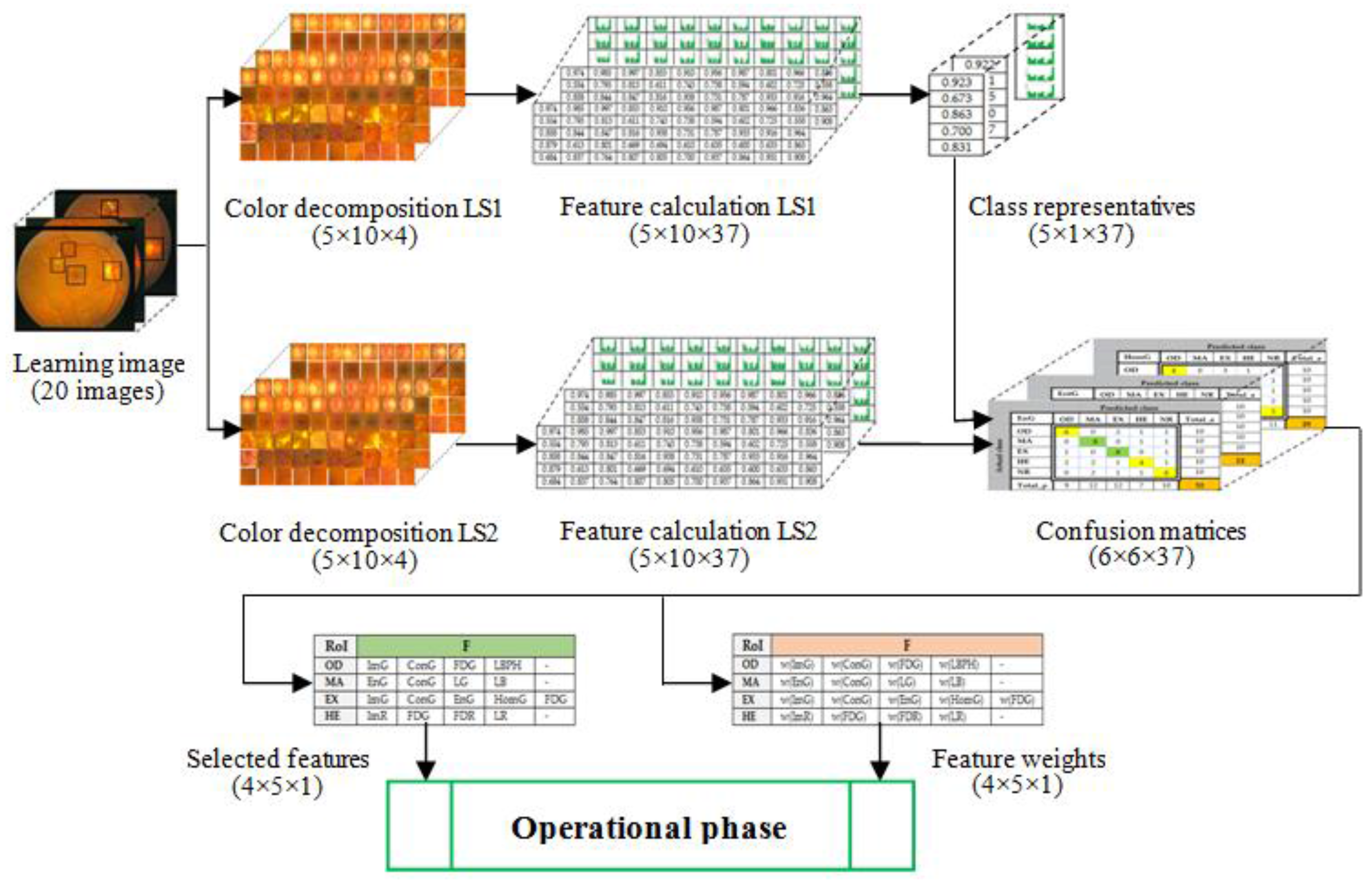
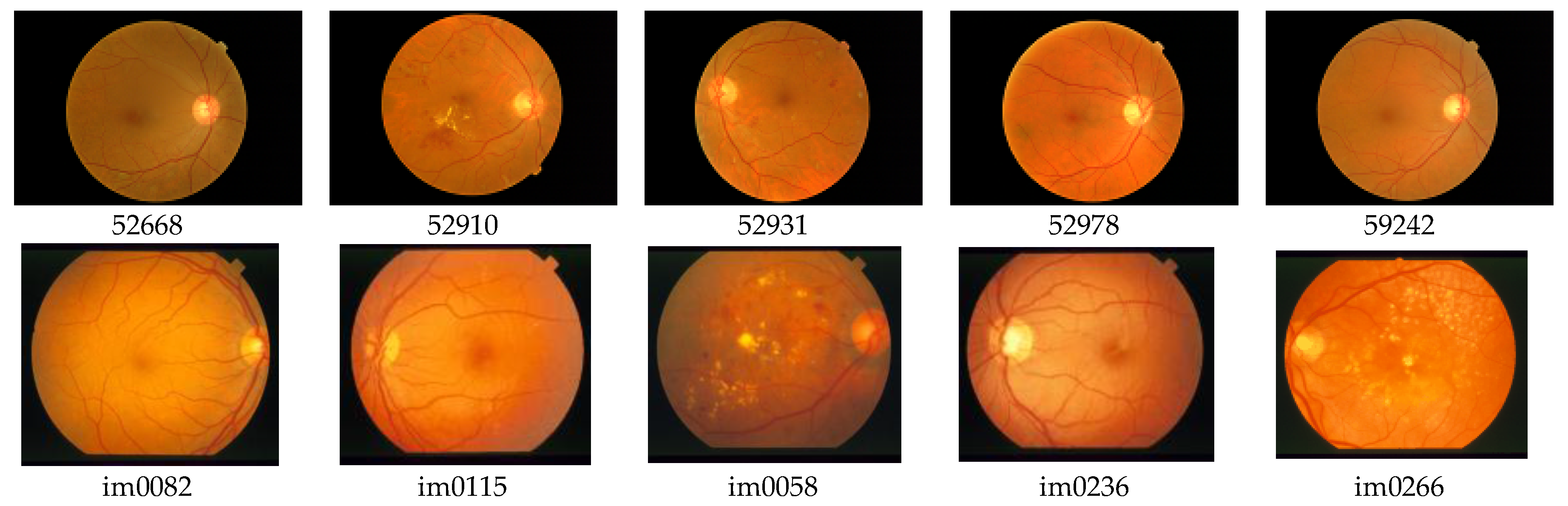
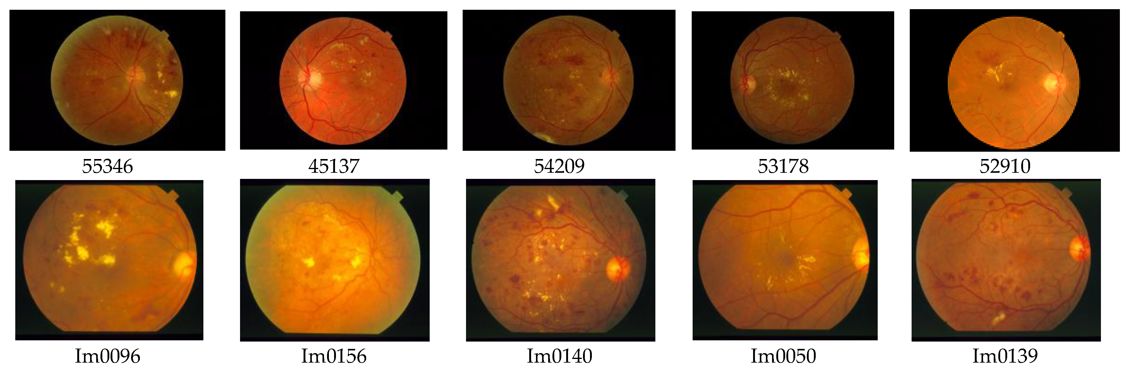
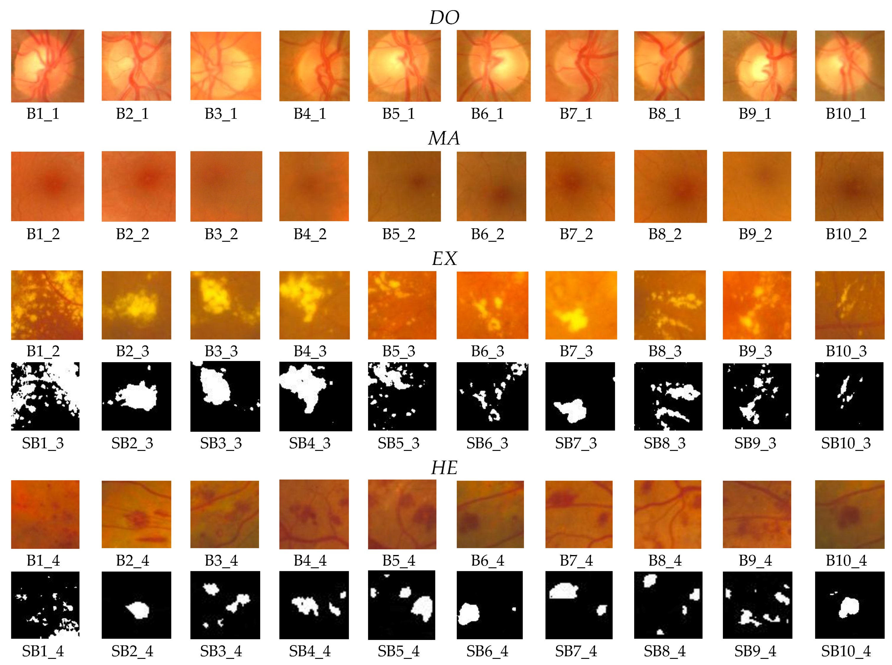
For the testing and validation of the proposed sensor we used 100 boxes from 60 images (Figure 7) for the learning phase and 200 images for the operating phase. As mentioned in Section 2, 50 boxes (10 for OD, 10 for MA, 10 for EX, 10 for HE, and 10 for NR; Figure 8) were used in feature selection and another 50 boxes were used in classifier implementation. A box dimension of 128 × 128 pixels was used for STARE and a box dimension of 256 × 256 pixels was used for MESSIDOR. The sliding step sizes (BDS) were 10 pixels for the STARE DB and 15 pixels for the MESSIDOR DB. In BVS, the sliding step size was 1 pixel for both. The same features were selected both in the STARE case and the MESSIDOR case. Examples of feature calculations for OD class representations are presented in Table 2 (36 features) and Table 3 (LBP feature). The last column contains the average values of the row. The results concerning the representatives for the classes OD, MA, EX, and HE are presented in Table 4. The features from CF (Table 1) were tested on R, G, B, and H color components and, in concordance with the selection criterion, the selected features and the corresponding color channels are marked with green in Table 4.

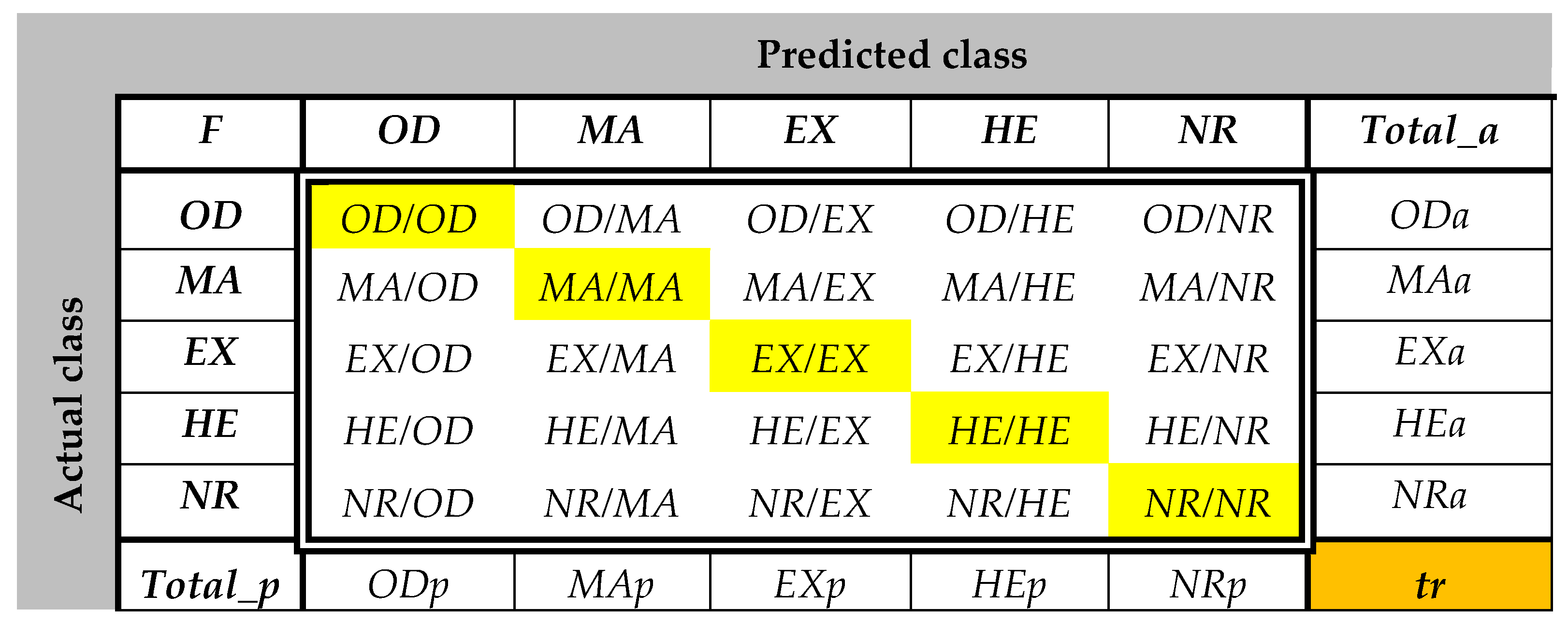
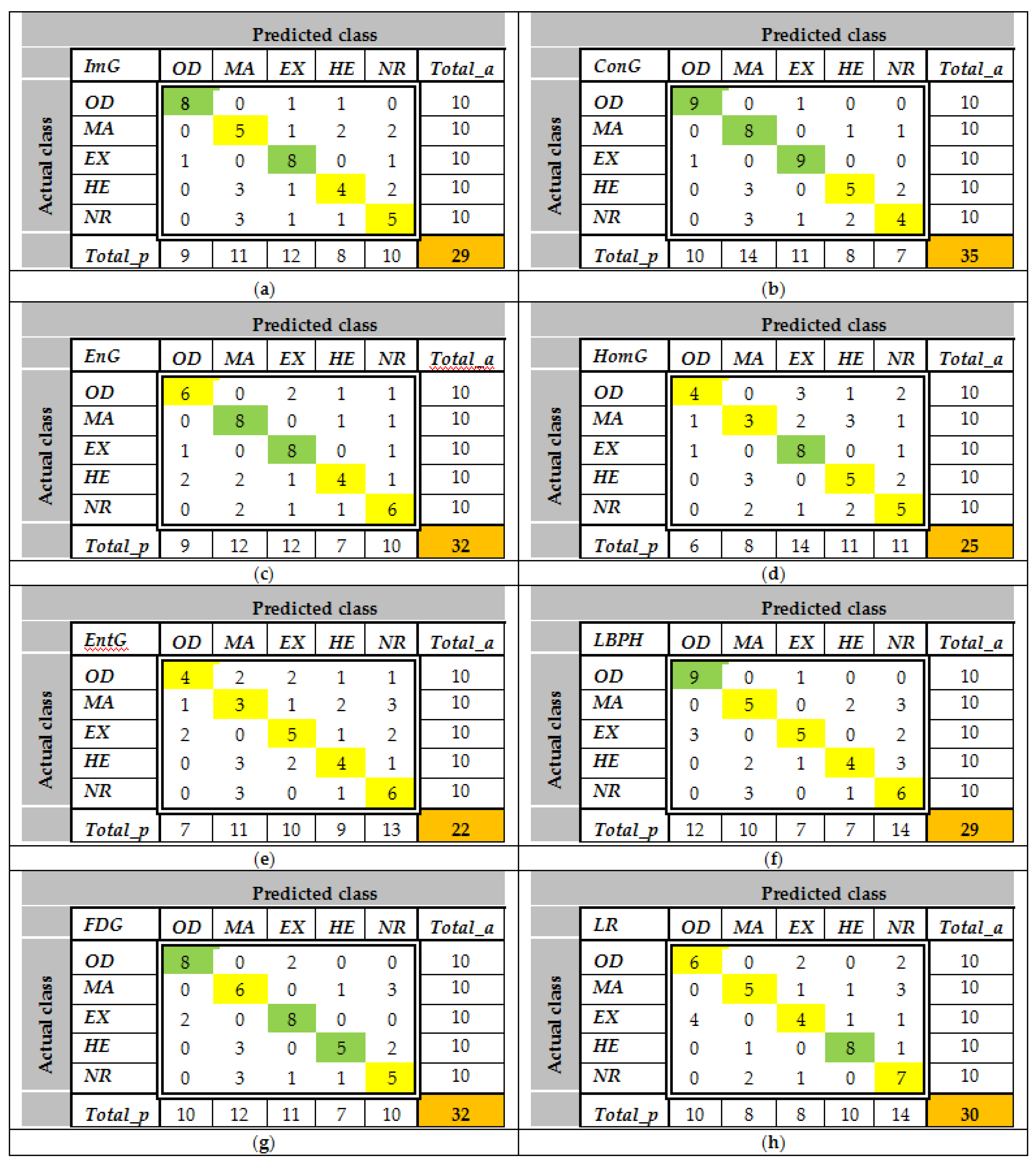
The confusion matrices are calculated using the set LS2 for all features and all classes. Some examples of CMs are presented in Figure 9. As can be observed, the values greater than 8 (greater than 0.75Cⁱa—see feature selection from the Section 2.3.2) are highlighted with green. For example, according to Figure 9a, ImG is a feature selected for OD and EX detection. Similarly, Figure 9b determines the classifiers which use ConG, Figure 9c determines the classifiers which use EnG, Figure 9d determines the classifiers which use HomG, Figure 9f determines the classifiers which use LBPH, Figure 9g determines the classifiers which use FDG, and Figure 9h determines the classifiers which use LR. It can be observed in Figure 9e that EntG is not a proper feature for any class.

Table 5 presents the traces of all confusion matrices associated with features (the rows represent such CM traces). The fulfillment of the selection criterion for the feature-class pair (from the confusion matrices) and also the associated weights for classifiers are highlighted in gray. The last column indicates the class which uses the corresponding feature in their classifier. The features and associated weights for each RoI can be extracted from Table 5. The classifiers from Equation (12)—D₁, D₂, D₃, and D₄—were implemented taking into account the confidence intervals and band associated with the weights and the corresponding RoIs (OD, MA, EX, and HE) (

Table 6. Results for class representatives.

Class	Selected Features	Weight	Values of the Class Representative. Confidence Intervals and Band (LBPH Case)
OD	ImG	0.8	[0.515; 0.594]
	ConG	0.9	[0.392; 0.476]
	FDG	0.8	[2.575; 2.613]
	LBPH	0.9	[11381; 13000], [5095; 5813], [5141; 5512], [1395; 1941], [5609; 6320], [5842; 7123], [1926; 2231], [5225; 5836], [5361; 6010], [14276; 15261]
MA	ConG	0.8	[0.038; 0.063]
	EnG	0.8	[0.701; 0.742]
	LG	0.8	[0.081; 0.113]
	LB	0.8	[0.049; 0.064]
EX	ImG	0.8	[0.431; 0.478]
	ConG	0.9	[0.575; 0.627]
	EnG	0.8	[0.789; 0.824]
	MomG	0.8	[0.852; 0.901]
	FDG	0.8	[2.491, 2.527]
HE	ImR	0.8	[0.679; 0.717]
	FDR	0.8	[2.487; 2.525]
	LR	0.8	[0.141; 0.163]
	LB	0.8	[0.103; 0.126]

). For the operational phase testing, both MESSIDOR and STARE databases were used (Figure 10). Some results concerning the box classification are given in Figure 11. The boxes classified as EX or HE have undergone a segmentation process (Figure 11, boxes labeled with SB). The results of size evaluation of EXs and HEs are presented in

Table 7. Area and percentage of EXs for different segmented boxes.

Box	SB1_3	SB2_3	SB3_3	SB4_3	SB5_3	SB6_3	SB7_3	SB8_3	SB9_3	SB10_3
Pixels	1819	713	776	957	608	366	420	543	389	129
Percent (%)	44.38	17.39	18.94	23.36	14.85	8.95	10.25	13.26	9.50	3.15

and

Table 8. Area and percentage of HEs for different segmented boxes.

Box	SB1_4	SB2_4	SB3_4	SB4_4	SB5_4	SB6_4	SB7_4	SB8_4	SB9_4	SB10_4
Pixels	406	249	307	355	453	353	416	242	350	264
Percent (%)	9.91	6.08	7.49	8.66	11.05	8.62	10.15	5.91	8.54	6.44

, respectively. Then, by summing the partial areas of EXs (HEs) from boxes belonging to the same image, a global evaluation in pixels and percent can be obtained (

Table 9. Segmented boxes with EX from the image Im0001 (STARE DB). Partial and total size and corresponding percentage.

Segmented Boxes/Entire Image
Area (pixels)	1757	1127	983	622	961	8683
Percentage (%)	42.9	27.5	24	15.18	23.46	3

).

4. Discussion

For testing and evaluation of the proposed system we used a set of 200 images from STARE and MESSIDOR databases (S1: 50 normal, without EX or HE; S2: 50 only with EX; S3: 50 only with HE; S4: 50 with both EX and HE). From S1, S2, S3, and S4, OD and MA were detected; from S2 and S4, EX was evaluated; and from S3 and S4, HE was evaluated. The flexibility of the system allows the use of different box dimensions for different databases. For box classification, the performances are presented in

Table 10. The confusion matrices and the performances for box classification.

RoI Performances	OD	MA	EX	HE
Precision (%) $PPV=\frac{TP}{TP+FP}$	99.5	98	97.5	97
Accuracy (%) $ACC=\frac{TP+TN}{TP+TN+FP+FN}$	99	98	98	96

, where TP is true positive, TN is true negative, FP is false positive, and FN is false negative. The obtained performances in terms of accuracy are presented and compared with other methods in

Table 11. Performance comparison (accuracy (%)).

Method RoI	[8]	[16]	[17]	[18]	[29]	[30]	[40]	[41]	[53]	[45]	Our Method
OD	91.36	98.77	95.77	99.2	-	-	-	-	-	-	99
MA	-	-	-	-	94	97.5	-	-	-	-	98
EX	-	-	-	-	-	-	97.01	93.8	85.6	-	98
HE	-	-	-	-	-	-	-	-	-	97.2	96

. It can be observed that only our system performs the detection of all RoIs and the results are similar to or better than those of other methods.

In this particular experiment the blood vessel analysis was not considered for OD detection as it has been detailed in a previous work by the authors [6]. By considering the pixel density of the blood vessels in the candidate boxes to contain OD, it was experimentally shown that the accuracy detection increased. Contrarily, by eliminating the blood vessels from the retinal image, HE detection and segmentation gave better results. As a direction for feature research, we propose to extend the system functions to other parameters like OD diameter, cup/OD diameter ratio, and blood vessel segmentation of an entire image.

5. Conclusions

The proposed method for the detection and evaluation of retinal RoIs takes into consideration information about pixel distribution (second-order statistics), color, and fractal textures. An intelligent system is thus implemented which contains three main modules: preprocessing, learning, and operating. The retinal images are decomposed into boxes (of variable size) for different RoIs, with the aid of a sliding box algorithm or a nonoverlapping box algorithm. Furthermore, a CNN structure is proposed for blood vessel segmentation. In the learning phase, effective feature selection is made based on the primary statistic information provided by confusion matrices and minimum distance classifiers. Two important cues are considered for the operational mode: weights given to the selected features and confidence intervals associated with the selected features for each class (representatives of classes). Conclusively, statistical analysis and comparison with similar works validated the implemented system.

References

1. Li, J.Q.; Welchowski, T.; Schmid, M.; Letow, J.; Wolpers, A.C.; Holz, F.G.; Finger, R.P. Retinal Diseases in Europe. Prevalence, Incidence and Healthcare Needs; EURETINA Report; EURETINA: Bonn, Germany, 2017. [Google Scholar]
2. Mohamed, N.A.; Zulkifley, M.A.; Hussain, A.; Mustapha, A. Local binary patterns and modified red channel for optic disc segmentation. J. Theor. Appl. Inf. Technol. 2015, 81, 84–91. [Google Scholar]
3. Mohammad, S.; Morris, D.T.; Thacker, N. Texture analysis for the segmentation of optic disc in retinal images. In Proceedings of the 2013 IEEE International Conference on Systems, Man, and Cybernetics, Manchester, UK, 13–16 October 2013; pp. 4265–4270. [Google Scholar] [CrossRef]
4. Popescu, D.; Ichim, L.; Caramihale, T. Computer—Aided localization of the optic disc based on textural features. In Proceedings of the 9th International Symposium on Advanced Topics in Electrical Engineering, Bucharest, Romania, 7–9 May 2015; pp. 307–312. [Google Scholar]
5. Mendonça, A.M.; Sousa, A.; Mendonça, L.; Campilho, A. Automatic localization of the optic disc by combining vascular and intensity information. Comput. Med. Imaging Graph. 2013, 37, 409–417. [Google Scholar] [CrossRef] [PubMed]
6. Ichim, L.; Popescu, D.; Cirneanu, S. Combining blood vessel segmentation and texture analysis to improve optic disc detection. In Proceedings of the 5th IEEE International Conference on E-Health and Bioengineering, Iaşi, Romania, 19–21 November 2015; pp. 1–4. [Google Scholar]
7. Qureshi, R.J.; Kovacs, L.; Harangi, B.; Nagy, B.; Peto, T.; Hajdu, A. Combining algorithms for automatic detection of optic disc and macula in fundus images. Comput. Vis. Image Underst. 2012, 116, 138–145. [Google Scholar] [CrossRef]
8. Dehghani, A.; Moghaddam, H.A.; Moin, M.-S. Optic disc localization in retinal images using histogram mathing. EURASIP J. Image Video Process. 2012, 2012, 19. [Google Scholar] [CrossRef]
9. Zhang, D.; Zhao, Y. Novel accurate and fast optic disc detection in retinal images with vessel distribution and directional characteristics. IEEE J. Biomed. Health Inform. 2016, 20, 333–342. [Google Scholar] [CrossRef] [PubMed]
10. Xiong, L.; Li, H. An approach to locate optic disc in retinal images with pathological changes. Comput. Med. Imaging Graph. 2016, 27, 40–50. [Google Scholar] [CrossRef] [PubMed]
11. Rahebi, J.; Hardalac, F. A new approach to optic disc detection in human retinal images using the firefly algorithm. Med. Biol. Eng. Comput. 2016, 54, 453–461. [Google Scholar] [CrossRef] [PubMed]
12. Dashtbozorga, B.; Mendonca, A.M.; Campilhoc, A. Optic disc segmentation using the sliding band filter. Comput. Biol. Med. 2015, 56, 1–12. [Google Scholar] [CrossRef] [PubMed]
13. Panda, R.; Puhan, N.B.; Panda, G. Global vessel symmetry for optic disc detection in retinal images. In Proceedings of the Fifth National Conference on Computer Vision, Pattern Recognition, Image Processing and Graphics (CVPRIPG 2015), Patna, Bihar, 16–19 December 2015; pp. 1–4. [Google Scholar] [CrossRef]
14. Giachetti, A.; Ballerini, L.; Trucco, E. Accurate and reliable segmentation of the optic disc in digital fundus images. J. Med. Imaging 2014, 1, 024001. [Google Scholar] [CrossRef] [PubMed] [Green Version]
15. El-Abbadi, N.K.; Al-Saadi, E.H. Automatic detection of exudates in retinal images. Int. J. Comput. Sci. Issues 2013, 10, 237–242. [Google Scholar]
16. Youssif, A.A.; Ghalwash, A.Z.; Ghoneim, A.S. Optic disc detection from normalized digital fundus images by means of a vessels’ direction matched filter. IEEE Trans. Med. Imaging 2008, 27, 11–18. [Google Scholar] [CrossRef] [PubMed]
17. Pereira, C.; Gonçalves, L.; Ferreira, M. Optic disc detection in color fundus images using ant colony optimization. Med. Biol. Eng. Comput. 2013, 51, 295–303. [Google Scholar] [CrossRef] [PubMed]
18. Alghamdi, H.S.; Tang, H.L.; Waheeb, S.A.; Peto, T. Automatic optic disk abnormality detection in fundus images: a deep learning approach. In Proceedings of the Medical Image Computing and Computer-Assisted Interventions—MICCAI 2016, Athens, Greece, 17–21 October 2016; Volume LNCS 9900, pp. 1–8. [Google Scholar] [CrossRef]
19. Cheng, J.; Wong, D.W.K.; Cheng, X.; Liu, J.; Tan, N.M.; Bhargava, M.; Cheung, C.M.G.; Wong, T.Y. Early age-related macular degeneration detection by focal biologically inspired feature. In Proceedings of the 19th IEEE International Conference on Image Processing, Orlando, FL, USA, 30 September–3 October 2012; pp. 2805–2808. [Google Scholar] [CrossRef]
20. Hijazi, M.H.A.; Coenen, F.; Zheng, Y. Data mining techniques for the screening of age-related macular degeneration. Knowl.-Based Syst. 2012, 29, 83–92. [Google Scholar] [CrossRef]
21. Zheng, Y.; Hijazi, M.H.A.; Coenen, F. Automated disease/no disease grading of age-related macular degeneration by an image mining approach. Investig. Ophthalmol. Vis. Sci. 2012, 53, 8310–8318. [Google Scholar] [CrossRef] [PubMed]
22. Köse, C.; Şevik, U.; Gençalioğlu, O.; İkibaş, C.; Kayıkıçıoğlu, T. A statistical segmentation method for measuring age-related macular degeneration in retinal fundus images. J. Med. Syst. 2010, 34, 1–13. [Google Scholar] [CrossRef] [PubMed]
23. Burlina, P.; Freund, D.E.; Joshi, N.; Wolfson, Y.; Bressler, N.M. Detection of age-related macular degeneration via deep learning. In Proceedings of the 13th IEEE International Symposium on Biomedical Imaging (ISBI 2016), Prague, Czech, 13–16 April 2016; pp. 184–188. [Google Scholar] [CrossRef]
24. Liang, Z.; Wong, D.W.K.; Liu, J.; Chan, K.L.; Wong, T.Y. Towards automatic detection of age-related macular degeneration in retinal fundus images. In Proceedings of the Annual International Conference of the IEEE Engineering in Medicine and Biology, Buenos Aires, Argentina, 31 August–4 September 2010; pp. 4100–4103. [Google Scholar] [CrossRef]
25. Veras, R.; Medeiros, F.; Silva, R.; Ushizima, D. Assessing the accuracy of macula detection methods in retinal images. In Proceedings of the 18th International Conference on Digital Signal Processing (DSP 2013), Santorini, Greece, 1–3 July 2013; pp. 1–6. [Google Scholar] [CrossRef]
26. Sekhar, S.; El-Samie, F.; Yu, P.; Al-Nuaimy, W.; Nandi, A. Automated localisation retinal features. Appl. Opt. 2011, 50, 3064–3075. [Google Scholar] [CrossRef] [PubMed]
27. Tan, N.M.; Wong, D.W.K.; Liu, J.; Ng, W.J.; Zhang, Z.; Lim, J.H.; Tan, Z.; Tang, Y.; Li, H.; Lu, S.; et al. Automatic detection of the macula in the retinal fundus image by detecting regions with low pixel intensity. In Proceedings of the International Conference on Biomedical and Pharmaceutical Engineering, (ICBPE’09), Singapore, 2–4 December 2009; pp. 1–5. [Google Scholar] [CrossRef]
28. Akram, M.U.; Tariq, A.; Khan, S.A.; Javed, M.Y. Automated detection of exudates and macula for grading of diabetic macular edema. Comput. Methods Programs Biomed. 2014, 114, 141–152. [Google Scholar] [CrossRef] [PubMed]
29. Chaudhry, A.R.; Bellmann, C.; Le Tien, V.; Klein, J.C.; Parra-Denis, E. Automatic macula detection in human eye fundus auto-fluorescence images: Application to eye disease localization. In Proceedings of the 10th European Congress of ISS, Milano, Italy, 26–29 June 2009; pp. 1–6. [Google Scholar]
30. Wong, D.W.; Liu, J.; Tan, N.M.; Yin, F.; Cheng, X.; Cheng, C.Y.; Cheung, G.C.; Wong, T.Y. Automatic detection of the macula in retinal fundus images using seeded mode tracking approach. In Proceedings of the Annual International Conference of the IEEE Engineering in Medicine and Biology Society (EMBC 2012), San Diego, CA, USA, 28 August–1 September 2012; pp. 4950–4953. [Google Scholar] [CrossRef]
31. Phillips, R.; Forrester, J.; Sharp, P. Automated detection and quantification of retinal exudates. Graefe’s Arch. Clin. Exp. Ophthalmol. 1993, 231, 90–94. [Google Scholar] [CrossRef]
32. Ege, B.; Hejlesen, O.; Larsen, O.; Moller, K.; Jennings, B.; Kerr, D.; Cavan, D. Screening for diabetic retinopathy using computer based image analysis and statistical classification. Comput. Meth. Programs Biomed. 2000, 62, 165–175. [Google Scholar] [CrossRef]
33. Usher, D.; Dumskyj, M.; Himaga, M.; Williamson, T.H.; Nussey, S.; Boyce, J. Automated detection of diabetic retinopathy in digital retinal images: A tool for diabetic retinopathy screening. Diabet. Med. 2004, 21, 84–90. [Google Scholar] [CrossRef] [PubMed]
34. Kaur, J.; Mittal, D. Segmentation and measurement of exudates in fundus images of the retina for detection of retinal disease. J. Biomed. Eng. Med. Imaging 2015, 2, 27–38. [Google Scholar] [CrossRef]
35. Bu, W.; Wu, X.; Chen, X.; Dai, B.; Zheng, Y. Hierarchical detection of hard exudates in color retinal images. J. Softw. 2013, 8, 2723–2732. [Google Scholar] [CrossRef]
36. Osareh, A.; Shadgar, B.; Markahm, R. A computational-intelligence-based approach for detection of exudates in diabetic retinopathy images. IEEE Trans. Inf. Technol. Biomed. 2009, 13, 535–545. [Google Scholar] [CrossRef] [PubMed]
37. Walter, T.; Klein, J.C.; Massin, P.; Erginay, A. A contribution of image processing to the diagnosis of diabetic retinopathy-detection of exudates in color fundus images of the human retina. IEEE Trans. Med. Imaging 2002, 21, 1236–1243. [Google Scholar] [CrossRef] [PubMed]
38. Seoud, L.; Hurtut, T.; Chelbi, J.; Cheriet, F.; Langlois, J.M.P. Red lesion detection using dynamic shape features for diabetic retinopathy screening. IEEE Trans. Med. Imaging 2016, 35, 1116–1126. [Google Scholar] [CrossRef] [PubMed]
39. Tang, L.; Niemeijer, M.; Joseph, M.; Reinhardt, J.M.; Garvin, M.K.; Abramoff, M.D. Splat feature classification with application to retinal hemorrhage detection in fundus images. IEEE Trans. Med. Imaging 2013, 32, 364–375. [Google Scholar] [CrossRef] [PubMed]
40. Garcia, M.; Sachez, C.I.; Lopez, M.I.; Abasolo, D.; Hornero, R. Neural network based detection of hard exudates in retinal images. Comput. Methods Programs Biomed. 2009, 93, 9–19. [Google Scholar] [CrossRef] [PubMed] [Green Version]
41. Garcia, M.; Valverde, C.; Lopez, M.I.; Poza, J.; Hornero, R. Comparison of logistic regression and neural network classifiers in the detection of hard exudates in retinal images. In Proceedings of the 35th Annual International Conference of the IEEE Engineering in Medicine and Biology Society, Osaka, Japan, 3–7 July 2013; pp. 5891–5894. [Google Scholar] [CrossRef]
42. Marin, D.; Aquino, A.; Gegundez-Arias, M.E.; Bravo, J.M. A new supervised method for blood vessel segmentation in retinal images by using gray-level and moment invariants-based features. IEEE Trans. Med. Imaging 2011, 30, 146–158. [Google Scholar] [CrossRef] [PubMed]
43. Hoover, A.; Goldbaum, M. Locating the optic nerve in a retinal image using the fuzzy convergence of the blood vessels. IEEE Trans. Med. Imaging 2003, 22, 951–958. [Google Scholar] [CrossRef] [PubMed]
44. Stall, J.J.; Abramoff, M.D.; Niemeijer, M.; Viergever, M.A.; van Ginneken, B. Ridge based vessel segmentation in color images of the retina. IEEE Trans. Med. Imaging 2004, 23, 501–509. [Google Scholar] [CrossRef] [PubMed]
45. Van Grinsven, M.J.J.P.; van Ginneken, B.; Hoyng, C.B.; Theelen, T.; Sanchez, C.I. Fast convolutional neural network training using selective data sampling: Application to hemorrhage detection in color fundus images. IEEE Trans. Med. Images 2016, 25, 1273–1284. [Google Scholar] [CrossRef] [PubMed]
46. Hajdu, A.; Hajdu, L.; Jonas, A.; Kovacs, L.; Toman, H. Generalizing the majority voting scheme to spatially constrained voting. IEEE Trans. Image Process. 2013, 22, 4182–4194. [Google Scholar] [CrossRef] [PubMed]
47. Decencière, E.; Zhang, X.; Cazuguel, G.; Lay, B.; Cochener, B.; Trone, C.; Gain, P.; Ordonez, R.; Massin, P.; Erginay, A.; et al. Feedback on a publicly distributed database: The Messidor database. Image Anal. Stereol. 2014, 33, 231–234. [Google Scholar] [CrossRef] [Green Version]
48. Caramihale, T.; Popescu, D.; Ichim, L. Interconnected neural networks based on voting scheme and local detectors for retinal image analysis and diagnosis. In Proceedings of the Image Analysis and Processing Conference—ICIAP 2017, Catania, Italy, Battiato, 11–15 September 2017; Gallo, G., Schettini, R., Stanco, F., Eds.; Lecture Notes in Computer Science. Volume 10485, pp. 753–764. [Google Scholar] [CrossRef]
49. Nayak, J.; Bhat, P.S.; Acharya, U.R.; Lim, C.M.; Kagathi, M. Automated identification of diabetic retinopathy stages using digital fundus images. J. Med. Syst. 2008, 32, 107–115. [Google Scholar] [CrossRef] [PubMed]
50. Nayak, J.; Acharya, U.R.; Bhat, P.S.; Shetty, N.; Lim, T.C. Automated diagnosis of glaucoma using digital fundus images. J. Med. Syst. 2009, 33, 337–346. [Google Scholar] [CrossRef] [PubMed]
51. Junior, S.B.; Welfer, D. Automatic detection of mycroaneurysms and hemorrhages in color eye fundus images. Int. J. Comput. Sci. Inf. Technol. 2013, 5, 21–37. [Google Scholar] [CrossRef]
52. Raja, D.S.S.; Vasuki, S. Screening diabetic retinopathy in developing countries using retinal images. Appl. Med. Inform. 2015, 36, 13–22. [Google Scholar]
53. Sopharak, A.; Uyyanonvara, B.; Barman, S. Automatic exudate detection from non-dilated diabetic retinopathy retinal images using fuzzy c-means clustering. Sensors 2009, 9, 2148–2161. [Google Scholar] [CrossRef] [PubMed]
54. Caramihale, T.; Popescu, D.; Ichim, L. Detection of regions of interest in retinal images using artificial neural networks and K-means clustering. In Proceedings of the International Conference on Applied Electromagnetics and Communications (ICECOM 2016), Dubrovnik, Croatia, 19–21 September 2016; pp. 1–6. [Google Scholar] [CrossRef]
55. Savu, M.; Popescu, D.; Ichim, L. Blood vessel segmentation in eye fundus images. In Proceedings of the International Conference on Smart Systems and Technologies (SST 2017), Osijek, Croatia, 18–20 October 2017; pp. 245–251. [Google Scholar] [CrossRef]
56. Haralick, R.M.; Shanmugam, K.; Dinstein, I.H. Textural features for image classification. IEEE Trans. Syst. Man Cybern. 1973, 6, 610–621. [Google Scholar] [CrossRef]
57. Sarkar, N.; Chaudhuri, B. An efficient differential box-counting approach to compute fractal dimension of image. IEEE Trans. Syst. Man Cybern. 1994, 24, 115–120. [Google Scholar] [CrossRef]
58. Barros Filho, M.N.; Sobreira, F.J.A. Accuracy of lacunarity algorithms in texture classification of high spatial resolution images from urban areas. In Proceedings of the XXI Congress of International Society of Photogrammetry and Remote Sensing (ISPRS 2008), Beijing, China, 3–11 July 2008; Part B3b. Volume XXXVII, pp. 417–422. [Google Scholar]
59. Ojala, T.; Pietikainen, M. Unsupervised texture segmentation using feature distributions. Pattern Recognit. 1999, 32, 477–486. [Google Scholar] [CrossRef]
60. Deza, M.-M.; Deza, E. Dictionary of Distances; Elsevier: Amsterdam, Netherlands, 2006. [Google Scholar]
Figure 1. Intelligent System for diagnosis and evaluation of regions of interest from Retinal Images concept (RoI – Region of Interest).
Symmetry 10 00073 g001
Figure 2. Exemplification of box division of the analyzed image: (a) sliding box algorithm; (b) nonoverlapping box algorithm.
Symmetry 10 00073 g002
Figure 3. Convolutional neural network (CNN)-based architecture of blood vessel segmentation (BVS).
Symmetry 10 00073 g003
Figure 4. Block diagram for the learning phase.
Symmetry 10 00073 g004
Figure 5. Confusion matrix (CM) for one feature F.
Symmetry 10 00073 g005
Figure 6. Block diagram for the operating phase (OP) and output module (included).
Symmetry 10 00073 g006
Figure 7. Examples of images from MESSIDOR (top) and STARE (bottom) databases for the learning phase.
Symmetry 10 00073 g007
Figure 8. Boxes of RoIs for feature calculation.
Symmetry 10 00073 g008
Figure 9. Examples of CM calculations and feature selection. Marked with green are the classes which accept the corresponding feature for the classifier.
Symmetry 10 00073 g009
Figure 10. Example of images from MESSIDOR (top) and STARE (bottom) databases for the operating phase.
Symmetry 10 00073 g010
Figure 11. Results of box classification.
Symmetry 10 00073 g011