Lie Symmetry of the Diffusive Lotka–Volterra System with Time-Dependent Coefficients

Abstract

Lie symmetry classification of the diffusive Lotka–Volterra system with time-dependent coefficients in the case of a single space variable is studied. A set of such symmetries in an explicit form is constructed. A nontrivial ansatz reducing the Lotka–Volterra system with correctly-specified coefficients to the system of ordinary differential equations (ODEs) and an example of the exact solution with a biological interpretation are found.

1. Introduction

It is widely known that A.J. Lotka and V. Volterra were the prominent investigators who created the mathematical background of ecology. Volterra proposed the classical model [1]

$$\begin{array}{c}\frac{du}{dt}=u(a-bv),\hfill \\ \frac{dv}{dt}=v(-c+du)\hfill \end{array}$$

(1)

for the predation of one species by another to explain the oscillatory levels of certain fish catches in the Adriatic. In (1), the functions $u\left(t\right)$ and $v\left(t\right)$ describe the time evolution of the numbers of prey and predators, respectively; the derivatives with respect to t represent the growth rates of the two populations over time; $a,b,c$ and d are positive real parameters describing the interaction of the two species. In words, one may formulate system (1) as follows [2]:

[Rate of change of u] = [net rate of growth of u without predation] − [net rate of loss of u due to predation],

[Rate of change of v] = − [net rate of loss of v without prey] + [net rate of growth of v due to predation].

Lotka proposed the same model [3] to describe chemical reaction, which exhibit periodic behaviour in the chemical concentrations. Thus, system (1) is known as the Lotka–Volterra model.

A natural generalization of system (1) follows if one takes into account diffusion of two species in a one-dimensional space. As a result, the diffusive Lotka–Volterra (DLV) system is obtained

$$\begin{array}{c}{u}_t=d_1{u}_{xx}+u(f_1+g_{1}u+h_{1}v),\hfill \\ v_t=d_2{v}_{xx}+v(f_2+g_{2}u+h_{2}v),\hfill \end{array}$$

(2)

where $f_i,g_i$ and $h_i$ are arbitrary constants ($i=1,2,$ $h_1^2+g_2^2\ne 0$), $d_1$ and $d_2$ are diffusion coefficients ($d_1{d}_2\ne 0$).

It is well-known that the DLV system (2) models several types of interaction between two populations of species. Three common types are the predator-prey interaction, the competition (for food, space, etc.) of species and mutualism. Each type of the species interaction is defined by coefficients’ signs in system (2). For example, the coefficients

$$f_i>0,g_i\le 0,h_i\le 0,i=1,2$$

are used in order to describe the competition, while the cases $h_1{g}_2<0$ and $h_1>0,$$g_2>0$ model the predator-prey interaction and mutualism, respectively (see (Chapter 3) [4] for details).

Nowadays many works (see, e.g., monograph (Chapter 3) [5] and papers [6,7,8,9,10,11]) are devoted to investigation of the DLV system (2) by analytical (in particular symmetry-based) methods. The existence of plane wave solutions of the DLV system (2) were examined in [6,7], while the works [8,9,10,11] are devoted to construct such solutions in an explicit forms. Note that the Lie symmetry classification problem for the DLV system (2) are completely solved in paper [8]. Moreover, such problem for the two-component reaction-diffusion system

$$\begin{array}{c}{u}_t=d_1{u}_{xx}+f\left(u,v\right),\hfill \\ v_t=d_2{v}_{xx}+g\left(u,v\right)\hfill \end{array}$$

(3)

(here $f(u,v)$ and $g(u,v)$ are the given smooth functions) was completed in paper [12].

In this paper, we examine a generalization of system (2) in the form

$$\begin{array}{c}{U}_{\tau }=D_1\left(\tau \right)U_{xx}+U\left(F_1\left(\tau \right)+G_1\left(\tau \right)U+H_1\left(\tau \right)V\right),\hfill \\ V_{\tau }=D_2\left(\tau \right)V_{xx}+V\left(F_2\left(\tau \right)+G_2\left(\tau \right)U+H_2\left(\tau \right)V\right),\hfill \end{array}$$

(4)

where $F_i,G_i,H_i$ and $D_i$ are arbitrary smooth functions ($H_1^2+G_2^2\ne 0,D_1{D}_2\ne 0$), and at least one of the coefficients of system (4) is not constant.

System (4) was investigated in many works (see, e.g., [13,14,15,16,17] and references cited therein). Chapter 2 of the book [13] is dedicated to some asymptotic stability questions concerning Lotka–Volterra type systems ($D_1=D_2=0$) with periodic coefficients, while other papers are devoted to examination the Lotka–Volterra type systems of the form (4) with $D_1{D}_2\ne 0$. However, to the best of our knowledge, there are no papers devoted to the search for the Lie symmetry of system (4).

The paper is organized as follows. In Section 2, the Lie symmetry classification of the DLV system with time-dependent coefficients is derived. In Section 3, the most important (from applicability point of view) cases of system (4) with nontrivial Lie symmetry are examined. In particular, a nontrivial Lie ansatz is derived and applied for reducing the system in question to a system of ODEs. The reduced systems are analyzed in order to construct exact solutions with a biological meaning. Finally, we briefly discuss the result obtained and present some conclusions in the last section.

2. Main Results

It can be noted that the DLV system (4) is reduced to the system

$$\begin{array}{c}{u}_t=u_{xx}+u\left(b_1\left(t\right)u+c_1\left(t\right)v\right),\hfill \\ v_t=d\left(t\right)v_{xx}+v\left(b_2\left(t\right)u+c_2\left(t\right)v\right)\hfill \end{array}$$

(5)

by the change of variables

$$t=\int D_1\left(\tau \right)d\tau ,u=U\exp \left(-\int F_1\left(\tau \right)d\tau \right),v=V\exp \left(-\int F_2\left(\tau \right)d\tau \right),$$

where $d\left(t\right)=\frac{D_2\left(\tau \right)}{D_1\left(\tau \right)},b_i\left(t\right)=\frac{G_i\left(\tau \right)}{D_1\left(\tau \right)}\exp \left(\int F_1\left(\tau \right)d\tau \right)$ and $c_i\left(t\right)=\frac{H_i\left(\tau \right)}{D_1\left(\tau \right)}\exp \left(\int F_2\left(\tau \right)d\tau \right),i=1,2,$ $\tau ={\left(\int D_1\left(t\right)dt\right)}^{-1}$ (the superscript $-1$ means inverse function).

In contrast to (4), the class of the DLV systems (5) contains only five arbitrary functions. Thus, the problem of a complete description of all possible Lie symmetries arises (one is also called group classification problem [18]). In order to solve this problem, we can apply the Lie–Ovsiannikov approach (the name of Ovsiannikov arises because he published a remarkable paper [19] in this direction). This approach is based on the classical Lie scheme and a set of equivalence transformations, which maps each system from one class to another one from this class.

Theorem 1.

An arbitrarily given DLV system of the form

$$\begin{array}{c}{U}_{\tau }=U_{yy}+U\left(G_1\left(\tau \right)U+H_1\left(\tau \right)V\right),\hfill \\ V_{\tau }=D\left(\tau \right)V_{yy}+V\left(G_2\left(\tau \right)U+H_2\left(\tau \right)V\right)\hfill \end{array}$$

(6)

can be reduced to a system from class (5) by the equivalence transformations of the form either

$$\begin{array}{c}t={\alpha }_1^2\tau +{\alpha }_2,x={\alpha }_{1}y+{\alpha }_3,\hfill \\ u={\alpha }_{4}U,v={\alpha }_{5}V,\hfill \\ d=D,b_1=\frac{G_1}{{\alpha }_4{\alpha }_1^2},b_2=\frac{G_2}{{\alpha }_4{\alpha }_1^2},c_1=\frac{H_1}{{\alpha }_5{\alpha }_1^2},c_2=\frac{H_2}{{\alpha }_5{\alpha }_1^2},\hfill \end{array}$$

(7)

or

$$\begin{array}{c}t={\alpha }_1^2\int D\left(\tau \right)d\tau +{\alpha }_2,x={\alpha }_{1}y+{\alpha }_3,\hfill \\ u={\alpha }_{4}V,v={\alpha }_{5}U,\hfill \\ d=\frac{1}{D},b_1=\frac{H_2}{{\alpha }_4{\alpha }_1^{2}D},b_2=\frac{H_1}{{\alpha }_4{\alpha }_1^{2}D},c_1=\frac{G_2}{{\alpha }_5{\alpha }_1^{2}D},c_2=\frac{G_1}{{\alpha }_5{\alpha }_1^{2}D},\hfill \end{array}$$

(8)

where ${\alpha }_j(j=1,\cdots ,5)$ are arbitrary constants such that ${\alpha }_1{\alpha }_4{\alpha }_5\ne 0.$

Sketch of the proof of Theorem 1.

Proof of this theorem is based on the direct method of constructing a group of equivalence transformations (see, e.g., [20]).

Let

$$\begin{array}{c}t=\alpha (\tau ,y,U,V),x=\beta (\tau ,y,U,V),\hfill \\ u=\mathsf{\Phi }(\tau ,y,U,V),v=\mathsf{\Psi }(\tau ,y,U,V)\hfill \end{array}$$

(9)

be an invertible smooth change of variables that transforms a system from class (6) into a system from (5).

First of all we note that for each nondegenerate change of variables (9) should satisfy the condition

$${\Delta }_1=\left|\begin{array}{cccc}{\alpha }_{\tau }& {\alpha }_y& {\alpha }_U& {\alpha }_V\\ {\beta }_{\tau }& {\beta }_y& {\beta }_U& {\beta }_V\\ {\mathsf{\Phi }}_{\tau }& {\mathsf{\Phi }}_y& {\mathsf{\Phi }}_U& {\mathsf{\Phi }}_V\\ {\mathsf{\Psi }}_{\tau }& {\mathsf{\Psi }}_y& {\mathsf{\Psi }}_U& {\mathsf{\Psi }}_V\end{array}\right|\ne 0.$$

(10)

The main idea of the proof is based on substituting the expressions for $U_{yy},V_{yy},U_{\tau },V_{\tau }$ (see formulae (9)) into system (6) and on analysis conditions when the system obtained is equivalent to (5).

The expressions for the first-order derivatives $U_{\tau }$ and $U_y$ have the form

$$\begin{array}{c}{U}_{\tau }=\frac{\left|\begin{array}{cc}{\mathsf{\Phi }}_{\tau }-{\alpha }_{\tau }{u}_t-{\beta }_{\tau }{u}_x& {\alpha }_V{u}_t+{\beta }_V{u}_x-{\mathsf{\Phi }}_V\\ {\mathsf{\Psi }}_{\tau }-{\alpha }_{\tau }{v}_t-{\beta }_{\tau }{v}_x& {\alpha }_V{v}_t+{\beta }_V{v}_x-{\mathsf{\Psi }}_V\end{array}\right|}{\left|\begin{array}{cc}{\alpha }_U{u}_t+{\beta }_U{u}_x-{\mathsf{\Phi }}_U& {\alpha }_V{u}_t+{\beta }_V{u}_x-{\mathsf{\Phi }}_V\\ {\alpha }_U{v}_t+{\beta }_U{v}_x-{\mathsf{\Psi }}_U& {\alpha }_V{v}_t+{\beta }_V{v}_x-{\mathsf{\Psi }}_V\end{array}\right|},\hfill \\ U_y=\frac{\left|\begin{array}{cc}{\mathsf{\Phi }}_y-{\alpha }_y{u}_t-{\beta }_y{u}_x& {\alpha }_V{u}_t+{\beta }_V{u}_x-{\mathsf{\Phi }}_V\\ {\mathsf{\Psi }}_y-{\alpha }_y{v}_t-{\beta }_y{v}_x& {\alpha }_V{v}_t+{\beta }_V{v}_x-{\mathsf{\Psi }}_V\end{array}\right|}{\left|\begin{array}{cc}{\alpha }_U{u}_t+{\beta }_U{u}_x-{\mathsf{\Phi }}_U& {\alpha }_V{u}_t+{\beta }_V{u}_x-{\mathsf{\Phi }}_V\\ {\alpha }_U{v}_t+{\beta }_U{v}_x-{\mathsf{\Psi }}_U& {\alpha }_V{v}_t+{\beta }_V{v}_x-{\mathsf{\Psi }}_V\end{array}\right|}.\hfill \end{array}$$

Since derivatives $V_{\tau }$ and $V_y$ have the same structure, the relevant formulae are omitted here.

The expressions for the second-order derivatives are very cumbersome and are skipped here. However, it can be noted that they contain the derivatives $u_{tt},v_{tt},u_{tx}$ and $v_{tx}$. Thus, the coefficient next to these derivatives must vanish, otherwise system (5) is not obtainable. These coefficients vanish if and only if the following equalities take place:

$${\alpha }_y={\alpha }_U={\alpha }_V={\beta }_U={\beta }_V=0\Rightarrow \alpha =\alpha \left(\tau \right),\beta =\beta (\tau ,y).$$

(11)

Moreover, taking into account (10), the restriction

$${\alpha }^{\prime }{\beta }_y\left|\begin{array}{cc}{\mathsf{\Phi }}_U& {\mathsf{\Phi }}_V\\ {\mathsf{\Psi }}_U& {\mathsf{\Psi }}_V\end{array}\right|\ne 0$$

(12)

is also obtained.

Having the set of equalities (11), the expressions for $U_{yy}$ and $U_{\tau }$ can be essentially simplified, namely:

$$\begin{array}{c}{U}_{yy}={\displaystyle \frac{{\mathsf{\Psi }}_V{\beta }_y^2}{{\Delta }_2}}{u}_{xx}-{\displaystyle \frac{{\mathsf{\Phi }}_V{\beta }_y^2}{{\Delta }_2}}{v}_{xx}+{\displaystyle \frac{{\left({\mathsf{\Psi }}_V{\beta }_y\right)}_y{\Delta }_2-{\left({\Delta }_2\right)}_y{\mathsf{\Psi }}_V{\beta }_y}{{\Delta }_2^2}}{u}_x-{\displaystyle \frac{{\left({\mathsf{\Phi }}_V{\beta }_y\right)}_y{\Delta }_2-{\left({\Delta }_2\right)}_y{\mathsf{\Phi }}_V{\beta }_y}{{\Delta }_2^2}}{v}_x+\hfill \\ {\displaystyle \frac{{({\mathsf{\Psi }}_y{\mathsf{\Phi }}_V-{\mathsf{\Psi }}_V{\mathsf{\Phi }}_y)}_y{\Delta }_2-{\left({\Delta }_2\right)}_y({\mathsf{\Psi }}_y{\mathsf{\Phi }}_V-{\mathsf{\Psi }}_V{\mathsf{\Phi }}_y)}{{\Delta }_2^2}},\hfill \\ U_{\tau }=\frac{1}{{\Delta }_2}\left({\mathsf{\Psi }}_V({\alpha }^{\prime }{u}_t+{\beta }_{\tau }{u}_x-{\mathsf{\Phi }}_{\tau })-{\mathsf{\Phi }}_V({\alpha }^{\prime }{v}_t+{\beta }_{\tau }{v}_x-{\mathsf{\Psi }}_{\tau })\right),\hfill \end{array}$$

(13)

where ${\Delta }_2=\left|\begin{array}{cc}{\mathsf{\Phi }}_U& {\mathsf{\Phi }}_V\\ {\mathsf{\Psi }}_U& {\mathsf{\Psi }}_V\end{array}\right|.$ Substituting (13) into the first equation of (6) we note that the expression obtained contains the terms

$$-\frac{{\mathsf{\Phi }}_V{\alpha }^{\prime }}{{\Delta }_2}\left(\frac{{\beta }_y^2}{{\alpha }^{\prime }}{v}_{xx}-v_t\right)\mathtt{and}\frac{{\mathsf{\Psi }}_V{\alpha }^{\prime }}{{\Delta }_2}\left(\frac{{\beta }_y^2}{{\alpha }^{\prime }}{u}_{xx}-u_t\right),$$

while other terms do not depend on $v_{xx},u_{xx},v_t,$ and $u_t.$

Now one realizes that there are two possibilities. Case $\left(\mathbf{i}\right)$: the first equation of (6) is transformed into the first one of (5). As a result, we obtain

$${\alpha }^{\prime }={\beta }_y^2,{\mathsf{\Phi }}_V=0.$$

(14)

In this case, the second equation of (6) is transformed into the second one of (5) and the following conditions

$$d=D,{\mathsf{\Psi }}_U=0$$

(15)

take place.

Case $\left(\mathbf{ii}\right)$: the first equation of (6) is transformed into the second one of (5). As a result, the conditions

$$d{\alpha }^{\prime }={\beta }_y^2,{\mathsf{\Psi }}_V=0,d=\frac{1}{D},{\mathsf{\Phi }}_U=0$$

must be satisfied.

Here we consider in detail only Case $\left(\mathbf{i}\right)$. Taking into account (12) and ${\mathsf{\Phi }}_V=0$, the restriction ${\mathsf{\Phi }}_U{\mathsf{\Psi }}_V\ne 0$ springs up.

On the other hand,

$$\beta (\tau ,y)={\beta }_1\left(\tau \right)y+{\beta }_2\left(\tau \right),$$

(16)

(here ${\beta }_1$ and ${\beta }_2$ are arbitrary smooth functions) follows from (14).

Substituting (14) and (15) into expressions for $U_{yy}$ and $U_{\tau }$ (see formulae (13)), one obtains

$$\begin{array}{c}{U}_{yy}={\displaystyle \frac{{\beta }_1^2}{{\mathsf{\Phi }}_U}}{u}_{xx}-2{\displaystyle \frac{{\beta }_1{\mathsf{\Phi }}_{yU}}{{\mathsf{\Phi }}_U^2}}{u}_x+{\displaystyle \frac{2{\mathsf{\Phi }}_y{\mathsf{\Phi }}_{yU}-{\mathsf{\Phi }}_U{\mathsf{\Phi }}_{yy}}{{\mathsf{\Phi }}_U^2}}-{\displaystyle \frac{{\mathsf{\Phi }}_{UU}}{{\mathsf{\Phi }}_U^3}}{({\beta }_1{u}_x-{\mathsf{\Phi }}_y)}^2,\hfill \\ U_{\tau }={\displaystyle \frac{1}{{\mathsf{\Phi }}_U}}({\beta }_1^2{u}_t+({\beta }_1^{\prime }y+{\beta }_2^{\prime })u_x-{\mathsf{\Phi }}_{\tau }).\hfill \end{array}$$

(17)

Since the first equation of system (5) does not contain the terms $u_x$ and $u_x^2$, the relevant coefficient should vanish, namely:

$$\begin{array}{c}2{\displaystyle \frac{{\beta }_1{\mathsf{\Phi }}_{yU}}{{\mathsf{\Phi }}_U^2}}+{\displaystyle \frac{{\beta }_1^{\prime }y+{\beta }_2^{\prime }}{{\mathsf{\Phi }}_U}}=0,\hfill \\ {\mathsf{\Phi }}_{UU}=0.\hfill \end{array}$$

The general solution of this system can be easily constructed and has the form

$$\mathsf{\Phi }=f\left(\tau \right)\exp \left(-{\displaystyle \frac{1}{4{\beta }_1}}({\beta }_1^{\prime }{y}^2+2{\beta }_2^{\prime }y)\right)U+P(\tau ,y),$$

(18)

where $f\left(\tau \right)\ne 0$ and $P(\tau ,y)$ are arbitrary functions. Thus, taking into account (9), (16) and (18), one can express the function U via the function u, namely:

$$U={\displaystyle \frac{u-P}{f}}\exp \left({\displaystyle \frac{{\beta }_1^{\prime }{(x-{\beta }_2)}^2}{4{\beta }_1^3}}+{\displaystyle \frac{{\beta }_2^{\prime }(x-{\beta }_2)}{2{\beta }_1^2}}\right).$$

(19)

Substituting (17)–(19) into the first equation of system (6), we obtain the term

$${\displaystyle \frac{G_1}{f{\beta }_1^2}}\exp \left({\displaystyle \frac{{\beta }_1^{\prime }{(x-{\beta }_2)}^2}{4{\beta }_1^3}}+{\displaystyle \frac{{\beta }_2^{\prime }(x-{\beta }_2)}{2{\beta }_1^2}}\right)u^2,$$

while other terms don’t contain $u^2$. Since the coefficients of system (5) do not depend on the variable x, we arrive at

$${\beta }_1^{\prime }=0\Rightarrow {\beta }_1={\alpha }_1,{\beta }_2^{\prime }=0\Rightarrow {\beta }_2={\alpha }_3,$$

where ${\alpha }_1\ne 0$ and ${\alpha }_3$ are arbitrary constants. Now we find $\alpha \left(\tau \right)={\alpha }_1^2\tau +{\alpha }_2$ from the first equation of (14). Therefore, the transformations for the variables t and x presented in (7) are obtained. As a result, the structure of the functions $\mathsf{\Phi }$ and $\mathsf{\Psi }$ are essentially simplified, namely:

$$\mathsf{\Phi }=f\left(\tau \right)U+P(\tau ,y),\mathsf{\Psi }=g\left(\tau \right)V+Q(\tau ,y),$$

(20)

where $g\left(\tau \right)\ne 0$ and $Q(\tau ,y)$ are arbitrary functions. Thus, the expressions for the derivatives $U_{\tau },V_{\tau },U_{yy}$ and $V_{yy}$ have the forms:

$$\begin{array}{c}{U}_{\tau }=\frac{1}{f}\left({\alpha }_1^2{u}_t-\frac{u-P}{f}{f}^{\prime }-P_{\tau }\right),U_{yy}=\frac{1}{f}\left({\alpha }_1^2{u}_{xx}-P_{yy}\right),\hfill \\ V_{\tau }=\frac{1}{g}\left({\alpha }_1^2{v}_t-\frac{v-Q}{g}{g}^{\prime }-Q_{\tau }\right),V_{yy}=\frac{1}{g}\left({\alpha }_1^2{v}_{xx}-Q_{yy}\right).\hfill \end{array}$$

(21)

Substituting (20) and (21) into (6), we arrive at the system

$$\begin{array}{c}{u}_t=u_{xx}+(u-P)\left({\displaystyle \frac{G_1}{{\alpha }_1^{2}f}}(u-P)+{\displaystyle \frac{H_1}{{\alpha }_1^{2}g}}(v-Q)\right)+{\displaystyle \frac{u-P}{{\alpha }_1^{2}f}}{f}^{\prime }+{\displaystyle \frac{P_{\tau }-P_{yy}}{{\alpha }_1^2}},\hfill \\ v_t=D{v}_{xx}+(v-Q)\left({\displaystyle \frac{G_2}{{\alpha }_1^{2}f}}(u-P)+{\displaystyle \frac{H_2}{{\alpha }_1^{2}g}}(v-Q)\right)+{\displaystyle \frac{v-Q}{{\alpha }_1^{2}g}}{g}^{\prime }+{\displaystyle \frac{Q_{\tau }-Q_{yy}}{{\alpha }_1^2}},\hfill \end{array}$$

which coincides with system (5) if the restrictions

$$P=Q=0,f^{\prime }=0\Rightarrow f={\alpha }_4,g^{\prime }=0\Rightarrow g={\alpha }_5$$

and the notations

$$d=D,b_1={\displaystyle \frac{G_1}{{\alpha }_4{\alpha }_1^2}},b_2={\displaystyle \frac{G_2}{{\alpha }_4{\alpha }_1^2}},c_1={\displaystyle \frac{H_1}{{\alpha }_5{\alpha }_1^2}},c_2={\displaystyle \frac{H_2}{{\alpha }_5{\alpha }_1^2}}$$

hold (here ${\alpha }_4\ne 0$ ${\alpha }_5\ne 0$ are arbitrary constants). Thus, the equivalence transformations of the form (7) are derived.

The examination of Case $\left(\mathbf{ii}\right)$ is quite similar and leads to the equivalence transformations of the form (8). ☐

It is well-known that the Lie–Ovsiannikov approach leads to very long list of equations (systems) with nontrivial Lie symmetry provided the given equation (system) contains several arbitrary functions (system (5) involves five such). Applying this approach to the DLV system (5), we obtain 51 inequivalent systems (up to equivalent representations generated by transformations of the form (7) and (8)). To essentially reduce the number of inequivalent systems, we use the algorithm based on so called form-preserving (admissible) transformations [21,22,23] (local substitutions, which can map some systems from a given class to other those belonging to the same class). During recent years, the application of admissible transformations to the Lie symmetry classification problems becomes more common because it enables one to decrease substantially the number of obtained cases [24,25,26,27] (see also an extensive discussion on this matter in the very recent monograph [28]). Here, this approach will be essentially used because the Lie–Ovsiannikov approach leads to many locally-equivalent systems of the form (5).

We start from a preliminary analysis of so-called determining equations. Applying the criterion of Lie’s invariance (see monographs and textbooks [18,28,29,30,31]) and making a preliminary analysis of the system of determining equations (DEs), we obtain the general form of the Lie symmetry operator of the DLV system (5).

Theorem 2.

Each invariance operator of any system from the class (5) has the following form:

$$\begin{array}{c}X={\xi }^0\left(t\right){\partial }_t+{\xi }^1(t,x){\partial }_x+\left(r^1(t,x)u+q^1\left(t\right)v+p^1(t,x)\right){\partial }_u+\hfill \\ \left(r^2(t,x)v+q^2\left(t\right)u+p^2(t,x)\right){\partial }_v,\hfill \end{array}$$

(22)

where ${\xi }^0,{\xi }^1,r^i,q^i$ and $p^i$ ($i=1,2$) are unknown smooth functions, which can be found from the system

$$\begin{array}{c}{d}^{\prime }\left(t\right){\xi }^0=0,\hfill \end{array}$$

(23)

$$\begin{array}{c}(1-d)q^1=0,(1-d)q^2=0,\hfill \end{array}$$

(24)

$$\begin{array}{c}(c_1-c_2)q^1=0,(b_1-b_2)q^2=0,\hfill \end{array}$$

(25)

$$\begin{array}{c}{\xi }_t^0-2{\xi }_x^1=0,{\xi }_t^1+2r_x^1=0,{\xi }_t^1+2d{r}_x^2=0,\hfill \end{array}$$

(26)

$$\begin{array}{c}{b}_1(r^1+{\xi }_t^0)+c_1{q}^2+{\xi }^0{b}_1^{\prime }=0,b_2(r^1+{\xi }_t^0)+(2c_2-c_1)q^2+{\xi }^0{b}_2^{\prime }=0,\hfill \end{array}$$

(27)

$$\begin{array}{c}{c}_1(r^2+{\xi }_t^0)+(2b_1-b_2)q^1+{\xi }^0{c}_1^{\prime }=0,c_2(r^2+{\xi }_t^0)+b_2{q}^1+{\xi }^0{c}_2^{\prime }=0,\hfill \end{array}$$

(28)

$$\begin{array}{c}{r}_t^1-r_{xx}^1-2b_1{p}^1-c_1{p}^2=0,r_t^2-d{r}_{xx}^2-b_2{p}^1-2c_2{p}^2=0,\hfill \end{array}$$

(29)

$$\begin{array}{c}{p}_t^1-p_{xx}^1=0,p_t^2-d{p}_{xx}^2=0,\hfill \end{array}$$

(30)

$$\begin{array}{c}{q}_t^1-c_1{p}^1=0,q_t^2-b_2{p}^2=0.\hfill \end{array}$$

(31)

Since the proof of this theorem is based on the known facts from Lie symmetry analysis and does not contain nontrivial steps, we omit the relevant calculations.

Obviously, the DLV system (5) for arbitrary functions $b_i,c_i$ and d admits the one-dimensional Lie algebra, called a principal (trivial) algebra, with the basic operator ${\partial }_x.$ To find all possible extensions of the principal algebra in the case of system (5), one needs to solve the system of DEs (23)–(31).

We present the result of integration of system (23)–(31) with the additional restriction $q^1{q}^2=0$ in the form of the theorem, which is the main result of the paper.

Theorem 3.

All possible maximal algebras of invariance (up to equivalent representations generated by transformations of the form (7) and (8)) with the restriction $q^1{q}^2=0$ of the DLV system (5) are presented in Table 1 and Table 2. Any other system of the form (6) with nontrivial Lie symmetry is reduced by a local substitution of the form

$$\begin{array}{c}t={\alpha }_1^2\tau +{\alpha }_2,x={\alpha }_{1}y+{\alpha }_3,\hfill \\ u={\alpha }_4{e}^{{\alpha }_{5}t}{f}^{{\alpha }_6}{g}^{{\alpha }_7}U+{\alpha }_{8}V+{\alpha }_9{e}^{{\alpha }_{10}t}{f}^{{\alpha }_{11}}{g}^{{\alpha }_{12}},\hfill \\ v={\alpha }_{13}\exp \left({\alpha }_{14}t+{\alpha }_{15}{e}^{{\alpha }_{16}t}\right)f^{{\alpha }_{17}}{g}^{{\alpha }_{18}}V+{\alpha }_{19}{e}^{{\alpha }_{20}t}{f}^{{\alpha }_{21}}{g}^{{\alpha }_{22}}U+{\alpha }_{23}{f}^{{\alpha }_{24}}{g}^{{\alpha }_{25}}\hfill \end{array}$$

(32)

either to one of those given in Table 1 and Table 2, or to the DLV system with constant coefficients, or to a correctly-specified reaction-diffusion system of the form (3). Here, the functions f and g take one of the following forms:

$$\tau ,\sin (\tau +{\alpha }_{26}),\sinh \left({\alpha }_{27}\ln \tau +{\alpha }_{28}\tau \right),\cosh \left({\alpha }_{29}\ln \tau +{\alpha }_{30}\tau \right),$$

while the constants α with subscripts are determined by the form of the system in question.

Table 1. Lie symmetries of system (5) with arbitrary d.

	d	Reaction Terms	Basic Operators of Maximal Algebra of Invariance
1.	$d\left(t\right)$	$b_1\left(t\right)u^2$	${\partial }_x,v{\partial }_v$
		$b_2\left(t\right)uv$
2.	$d\left(t\right)$	0	${\partial }_x,v{\partial }_v,{\partial }_u+\int b\left(t\right)dtv{\partial }_v$
		$b\left(t\right)uv$
3.	$d_0$	$u\left({\beta }_1{t}^{k}u+{\gamma }_1{t}^{l}v\right)$	${\partial }_x,2t{\partial }_t+x{\partial }_x-2(k+1)u{\partial }_u-2(l+1)v{\partial }_v$
		$v\left({\beta }_2{t}^{k}u+{\gamma }_2{t}^{l}v\right)$
4.	$d_0$	$\beta t^k{u}^2$	${\partial }_x,2t{\partial }_t+x{\partial }_x-2(k+1)u{\partial }_u,v{\partial }_v$
		$t^{k}uv$
5.	$d_0$	0	${\partial }_x,2t{\partial }_t+x{\partial }_x-2(k+1)u{\partial }_u,v{\partial }_v,{\partial }_u+\int t^{k}dtv{\partial }_v$
		$t^{k}uv$
6.	$d_0$	0	${\partial }_x,2t{\partial }_t+x{\partial }_x-2\left((k+1)u+\beta {(k+1)}^2\right){\partial }_u-$
		$v\left(t^{k}u+t^l\exp \left(\beta t^{k+1}\right)v\right)$	$2\left(l+1+\beta (k+1)t^{k+1}\right)v{\partial }_v$
7.	$d_0$	0	${\partial }_x,2t{\partial }_t+x{\partial }_x-4\beta {\partial }_u-2\left(l+1+2\beta \ln t\right)v{\partial }_v$
		$v\left(t^{-1}u+t^l\exp \left(\beta {\ln }^{2}t\right)v\right)$
8.	$d_0$	$t^{-1}{cos}^{-2}\left(k\ln t\right)u^2$	${\partial }_x,2t{\partial }_t+x{\partial }_x-2k(k+2\tan \left(k\ln t\right)u){\partial }_u-$
		$v\left({\displaystyle \frac{\beta t^{-1}}{{cos}^2\left(k\ln t\right)}}u+{\displaystyle \frac{t^l}{{cos}^{\beta }\left(k\ln t\right)}}v\right)$	$2\left(l+1+k\beta \tan \left(k\ln t\right)\right)v{\partial }_v$
9.	$d_0$	$t^{-1}{cos}^{-2}\left(k\ln t\right)u^2$	${\partial }_x,v{\partial }_v,2t{\partial }_t+x{\partial }_x-2k(k+2\tan \left(k\ln t\right)u){\partial }_u-$
		$\beta t^{-1}{cos}^{-2}\left(k\ln t\right)uv$	$2k\beta \tan \left(k\ln t\right)v{\partial }_v$
10.	$d_0$	$t^{-1}{\cosh }^{-2}\left(k\ln t\right)u^2$	${\partial }_x,2t{\partial }_t+x{\partial }_x+2k(k+2\tanh \left(k\ln t\right)u){\partial }_u-$
		$v\left({\displaystyle \frac{\beta t^{-1}}{{\cosh }^2\left(k\ln t\right)}}u+\frac{t^l}{{\cosh }^{\beta }\left(k\ln t\right)}v\right)$	$2\left(l+1-k\beta \tanh \left(k\ln t\right)\right)v{\partial }_v$
11.	$d_0$	$t^{-1}{\cosh }^{-2}\left(k\ln t\right)u^2$	${\partial }_x,v{\partial }_v,2t{\partial }_t+x{\partial }_x+2k(k+2\tanh \left(k\ln t\right)u){\partial }_u+$
		$\beta t^{-1}{\cosh }^{-2}\left(k\ln t\right)uv$	$2k\beta \tanh \left(k\ln t\right)v{\partial }_v$
12.	$d_0$	$t^{-1}{\ln }^{-2}t{u}^2$	${\partial }_x,2t{\partial }_t+x{\partial }_x+2(-1+2{\ln }^{-1}tu){\partial }_u+$
		$v\left(\beta t^{-1}{\ln }^{-2}tu+t^l{\ln }^{-\beta }tv\right)$	$2\left(\beta {\ln }^{-1}t-l-1\right)v{\partial }_v$
13.	$d_0$	$t^{-1}{\ln }^{-2}t{u}^2$	${\partial }_x,v{\partial }_v,2t{\partial }_t+x{\partial }_x+$
		$\beta t^{-1}{\ln }^{-2}tuv$	$2(-1+2{\ln }^{-1}tu){\partial }_u+2\beta {\ln }^{-1}tv{\partial }_v$

Table 2. Lie symmetries of system (5) with $d=1$.

	Reaction Terms	Basic Operators of Maximal Algebra of Invariance
1.	$u\left(t^k\ln tu+t^{k}v\right)$	${\partial }_x,2t{\partial }_t+x{\partial }_x-2(k+1)u{\partial }_u-2\left(u+(k+1)v\right){\partial }_v$
	$v\left(t^k\ln tu+t^{k}v\right)$
2.	$u\left({\displaystyle \frac{t^{k-1}(1-k\ln t)}{{\ln }^{2}t}}u+t^{-1}{\ln }^{-2}tv\right)$	${\partial }_x,2t{\partial }_t+x{\partial }_x+2\left({\ln }^{-1}t-k\right)u{\partial }_u+2\frac{2v+t^{k}u-\ln t}{\ln t}{\partial }_v$
	$v\left({\displaystyle \frac{t^{k-1}(1-k\ln t)}{{\ln }^{2}t}}u+t^{-1}{\ln }^{-2}tv\right)$
3.	$u\left({\displaystyle \frac{t^{k-1}\left(k+l\tan \left(l\ln t\right)\right)}{cos\left(l\ln t\right)}}u+{\displaystyle \frac{t^{-1}}{{cos}^2\left(l\ln t\right)}}v\right)$	${\partial }_x,2t{\partial }_t+x{\partial }_x-2\left(l\tan \left(l\ln t\right)+k\right)u{\partial }_u-$
	$v\left({\displaystyle \frac{t^{k-1}\left(k+l\tan \left(l\ln t\right)\right)}{cos\left(l\ln t\right)}}u+{\displaystyle \frac{t^{-1}}{{cos}^2\left(l\ln t\right)}}v\right)$	$2\left(2l\tan \left(l\ln t\right)v+{\displaystyle \frac{l^2{t}^k}{cos\left(l\ln t\right)}}u+l^2\right){\partial }_v$
4.	$u\left({\displaystyle \frac{t^{k-1}\left(k-l\tanh \left(l\ln t\right)\right)}{\cosh \left(l\ln t\right)}}u+{\displaystyle \frac{t^{-1}}{{\cosh }^2\left(l\ln t\right)}}v\right)$	${\partial }_x,2t{\partial }_t+x{\partial }_x+2\left(l\tanh \left(l\ln t\right)-k\right)u{\partial }_u+$
	$v\left({\displaystyle \frac{t^{k-1}\left(k-l\tanh \left(l\ln t\right)\right)}{\cosh \left(l\ln t\right)}}u+{\displaystyle \frac{t^{-1}}{{\cosh }^2\left(l\ln t\right)}}v\right)$	$2\left(2l\tanh \left(l\ln t\right)v+{\displaystyle \frac{l^2{t}^k}{\cosh \left(l\ln t\right)}}u+l^2\right){\partial }_v$
5.	$b\left(t\right)u^2$	${\partial }_x,u{\partial }_v,v{\partial }_v,(1+\int b\left(t\right)dtu){\partial }_v$
	$b\left(t\right)uv$
6.	$t^k{u}^2$	${\partial }_x,u{\partial }_v,v{\partial }_v,(1+\int t^{k}dtu){\partial }_v,$
	$t^{k}uv$	$2t{\partial }_t+x{\partial }_x-2(k+1)u{\partial }_u$
7.	$t^{-1}{cos}^{-2}\left(\beta \ln t\right)u^2$	${\partial }_x,u{\partial }_v,v{\partial }_v,(\beta +\tan \left(\beta \ln t\right)u){\partial }_v,$
	$t^{-1}{cos}^{-2}\left(\beta \ln t\right)uv$	$2t{\partial }_t+x{\partial }_x-2\beta \tan \left(\beta \ln t\right)v{\partial }_v-$
		$2({\beta }^2+2\beta \tan \left(\beta \ln t\right)u){\partial }_u$
8.	$t^{-1}{\cosh }^{-2}\left(\beta \ln t\right)u^2$	${\partial }_x,u{\partial }_v,v{\partial }_v,(\beta +\tanh \left(\beta \ln t\right)u){\partial }_v,$
	$t^{-1}{\cosh }^{-2}\left(\beta \ln t\right)uv$	$2t{\partial }_t+x{\partial }_x+2\beta \tanh \left(\beta \ln t\right)v{\partial }_v+$
		$2({\beta }^2+2\beta \tanh \left(\beta \ln t\right)u){\partial }_u$
9.	$t^{-1}{\ln }^{-2}t{u}^2$	${\partial }_x,u{\partial }_v,v{\partial }_v,(1-{\ln }^{-1}tu){\partial }_v,2t{\partial }_t+x{\partial }_x+$
	$t^{-1}{\ln }^{-2}tuv$	$2(-1+2{\ln }^{-1}tu){\partial }_u+2{\ln }^{-1}tv{\partial }_v$

Sketch of the proof of Theorem 3.

In order to prove the theorem, one needs to solve the system of DEs (23)–(31). The differential consequences of Equations (27) and (28) with respect to x lead to

$$b_i{r}_x^1=0,c_i{r}_x^2=0,i=1,2.$$

Since $c_1^2+b_2^2\ne 0$ (otherwise the DLV system (5) contains two independent equations, which are excluded from consideration) and taking into account (26), one arrives at

$$r_x^1=r_x^2=0,{\xi }^0=2{\alpha }_{2}t+{\alpha }_0,{\xi }^1={\alpha }_{2}x+{\alpha }_1,$$

where ${\alpha }_0,{\alpha }_1$ and ${\alpha }_2$ are arbitrary constants.

First of all, we note that two essentially different cases, $d^{\prime }\left(t\right)\ne 0$ and $d^{\prime }\left(t\right)=0$, follow from Equation (23).

Assuming $d^{\prime }\left(t\right)\ne 0$, Equations (23) and (24) immediately lead to

$${\xi }^0=q^1=q^2=0.$$

Under the above equalities Equations (27) and (28) essentially simplify and take the forms

$$b_i{r}^1=0,c_i{r}^2=0,i=1,2.$$

(33)

Thus, two different subcases should be examined : $\left(\mathbf{i}\right)$ $c_1{b}_2\ne 0$; $\left(\mathbf{ii}\right)$ $c_1=0,b_2\ne 0$. Formally speaking, there is a third subcase $b_2=0,c_1\ne 0$; however, it is equivalent to $\left(\mathbf{ii}\right)$ up to transformation (8).

Let us assume that $c_1{b}_2\ne 0$. Equations (31) and (33) immediately produce

$$r^1=r^2=p^1=p^2=0.$$

Thus, only the trivial algebra is obtained. The examination of subcase $\left(\mathbf{ii}\right)$ leads to Cases 1 and 2 of Table 1. Therefore, the case $d^{\prime }\left(t\right)\ne 0$ is completely examined.

Now we consider the case $d^{\prime }\left(t\right)=0.$ One notes from Equations (24) that two possibilities $d=d_0$ ($d_0$ is an arbitrary constant) and $d=1$ should be analysed. Here we examine in detail only the first possibility $d=d_0$.

Equations (24) lead to $q^1=q^2=0.$ The further analysis of the system of DEs depends on the functions $b_2$ and $c_1$. Thus, subcases $\left(\mathbf{i}\right)$ and $\left(\mathbf{ii}\right)$ should be considered.

Firstly, we note that ${\xi }^0\ne 0$ (otherwise only the trivial algebra or the particular subcases of Cases 1 and 2 of Table 1 are obtained).

Subcase $\left(\mathbf{i}\right)$. Equations (29) and (31) produce $p^1=p^2=0,r^1={\lambda }_1$ and $r^2={\lambda }_2,$ where ${\lambda }_1$ and ${\lambda }_2$ are arbitrary constants. Therefore, Equations (27) and (28) can be rewritten as

$$\begin{array}{c}{b}_1=b_0{b}_2,c_2=c_0{c}_1,\hfill \\ \frac{b_2^{\prime }}{b_2}=-\frac{{\lambda }_1+2{\alpha }_2}{2{\alpha }_{2}t+{\alpha }_0},\frac{c_1^{\prime }}{c_1}=-\frac{{\lambda }_2+2{\alpha }_2}{2{\alpha }_{2}t+{\alpha }_0}.\hfill \end{array}$$

(34)

Last two equations of system (34) can be easily integrated depending on the constant ${\alpha }_2.$ Thus, Case 3 of Table 1 is obtained provided ${\alpha }_2\ne 0$. If ${\alpha }_2=0$ the DLV system

$$\begin{array}{c}{u}_t=u_{xx}+u\left({\beta }_1{e}^{kt}u+{\gamma }_1{e}^{lt}v\right),\hfill \\ v_t=d_0{v}_{xx}+v\left({\beta }_2{e}^{kt}u+{\gamma }_2{e}^{lt}v\right)\hfill \end{array}$$

(35)

(here ${\beta }_i,{\gamma }_i,k$ and l are arbitrary constants, $k^2+l^2\ne 0$) and the relevant Lie symmetries

$${\partial }_x,{\partial }_t-ku{\partial }_u-lv{\partial }_v$$

(36)

are derived. Using the simple transformation $e^{kt}u\to u,e^{lt}v\to v$ to (35) and (36), we obtain the DLV system with constant coefficients

$$\begin{array}{c}{u}_t=u_{xx}+u\left(k+{\beta }_{1}u+{\gamma }_{1}v\right),\hfill \\ v_t=d_0{v}_{xx}+v\left(l+{\beta }_{2}u+{\gamma }_{2}v\right)\hfill \end{array}$$

and its trivial algebra $<{\partial }_x,{\partial }_t>.$ Therefore, subcase $\left(\mathbf{i}\right)$ is completely examined.

Subcase $\left(\mathbf{ii}\right)$. The system of DEs (23)–(31) takes the form:

$$\begin{array}{c}{r}_t^1=2\lambda b_1,r_t^2=\lambda b_2,\hfill \end{array}$$

(37)

$$\begin{array}{c}{b}_1(r^1+2{\alpha }_2)+(2{\alpha }_{2}t+{\alpha }_0)b_1^{\prime }=0,b_2(r^1+2{\alpha }_2)+(2{\alpha }_{2}t+{\alpha }_0)b_2^{\prime }=0,\hfill \end{array}$$

(38)

$$\begin{array}{c}{c}_2(r^2+2{\alpha }_2)+(2{\alpha }_{2}t+{\alpha }_0)c_2^{\prime }=0,\hfill \end{array}$$

(39)

and

$$p^1=\lambda ,p^2=0.$$

Note that system (37)–(39) can be easily integrated provided $\lambda b_1=0$ and eight different cases (up to equivalent transformations of the form (7) and (8)) are derived. Four of them (in which ${\alpha }_2=0$) are reduced to the DLV systems with constant coefficients by the form-preserving transformations of the form (32), while others are presented in Table 1 (see Cases 4–7).

Let us assume that $\lambda b_1\ne 0.$ Substituting the function $b_1=\frac{r_t^1}{2\lambda }$ into the first equation of (38), we arrive at the nonlinear second-order ODE

$$r_t^1(r^1+2{\alpha }_2)+(2{\alpha }_{2}t+{\alpha }_0)r_{tt}^1=0,$$

that can be rewritten as

$${\left((2{\alpha }_{2}t+{\alpha }_0)r_t^1\right)}_t+{\left(\frac{1}{2}{\left(r^1\right)}^2\right)}_t=0.$$

Integrating the above equation, we obtain

$$(2{\alpha }_{2}t+{\alpha }_0)r_t^1=-\frac{1}{2}\left({\left(r^1\right)}^2+\delta \right),$$

where $\delta$ is arbitrary constant. Depending on the constants ${\alpha }_2$ and $\delta$, one can find

$$r^1\left(t\right)=\left\{\begin{array}{c}\frac{2{\alpha }_0}{t},\mathrm{if}\delta =0,\hfill \\ \gamma \tan \left(-\frac{\gamma t}{2{\alpha }_0}\right),\mathrm{if}\delta ={\gamma }^2,\hfill \\ \gamma \tanh \left(\frac{\gamma t}{2{\alpha }_0}\right),\mathrm{if}\delta =-{\gamma }^2,\hfill \\ \gamma \coth \left(\frac{\gamma t}{2{\alpha }_0}\right),\mathrm{if}\delta =-{\gamma }^2,\hfill \end{array}\right.$$

(40)

if ${\alpha }_2=0$, and

$$r^1\left(t\right)=\left\{\begin{array}{c}\frac{4{\alpha }_2}{\ln t},\mathrm{if}\delta =0,\hfill \\ \gamma \tan \left(-\frac{\gamma \ln t}{4{\alpha }_2}\right),\mathrm{if}\delta ={\gamma }^2,\hfill \\ \gamma \tanh \left(\frac{\gamma \ln t}{4{\alpha }_2}\right),\mathrm{if}\delta =-{\gamma }^2,\hfill \\ \gamma \coth \left(\frac{\gamma \ln t}{4{\alpha }_2}\right),\mathrm{if}\delta =-{\gamma }^2,\hfill \end{array}\right.$$

(41)

if ${\alpha }_2\ne 0$, up to transformation $t\to t+t_0$. Having $r^1$ we find the functions $b_2,r^2$ and $c_2$ from the second equation of (38), the second equation of (37) and Equation (39), respectively. As a result, Cases 8–13 of Table 1 are derived. Note that all systems admitting Lie symmetry with the functions $r^1$ from (40) are reduced either to the DLV system with constant coefficients or to the reaction-diffusion system of the form (3). Moreover, the system corresponding to the last case of (41)

$$\begin{array}{c}{u}_t=u_{xx}+t^{-1}{\sinh }^{-2}\left(k\ln t\right)u^2,\hfill \\ v_t=d_0{v}_{xx}+v\left(\beta t^{-1}{\sinh }^{-2}\left(k\ln t\right)u+\delta t^l{\sinh }^{-\beta }\left(k\ln t\right)v\right),\hfill \end{array}$$

is reduced to the system from Cases 10 (if $\delta \ne 0$) and 11 (if $\delta =0$) of Table 1 by the form-preserving transformation

$$u\to {\tanh }^2\left(k\ln t\right)u+k\tanh \left(k\ln t\right),v\to {\tanh }^{\beta }\left(k\ln t\right)v.$$

Finally, to complete the proof we need to consider the possibility $d=1.$ If $q^1=q^2=0$ then we obtain Lie symmetry operators presented in Table 1. So, new results are obtainable only under the restriction ${\left(q^1\right)}^2+{\left(q^2\right)}^2\ne 0$. This restriction immediately leads to

$$b_1=b_2=b,c_1=c_2=c.$$

System (27)–(31) take the form:

$$\begin{array}{c}b(r^1+{\xi }_t^0)+c{q}^2+{\xi }^0{b}^{\prime }=0,\hfill \end{array}$$

(42)

$$\begin{array}{c}c(r^2+{\xi }_t^0)+b{q}^1+{\xi }^0{c}^{\prime }=0,\hfill \end{array}$$

(43)

$$\begin{array}{c}{r}_t^1=2{\lambda }_{1}b+{\lambda }_{2}c,r_t^2={\lambda }_{1}b+2{\lambda }_{2}c,\hfill \end{array}$$

(44)

$$\begin{array}{c}{q}_t^1={\lambda }_{1}c,q_t^2={\lambda }_{2}b\hfill \end{array}$$

(45)

and

$$p^1={\lambda }_1,p^2={\lambda }_2.$$

Note that we can integrate system (42)–(45) in general only for the semi-coupled DLV systems ($bc=0,b^2+c^2\ne 0$). Supposing $c=0$ and $b\ne 0$ (the case $c\ne 0,b=0$ is equivalent up to transformation (8)), one can obtain $q^1=0$ from Equation (43). As a result, Cases 5–9 of Table 2 were found.

In the case $bc\ne 0$, we cannot integrate system (42)–(45) in general. To solve this system we make additional restriction $q^1{q}^2=0$. Supposing $q^1=0,q^2\ne 0$ (the case $q^1\ne 0,q^2=0$ is equivalent up to transformation (8)), we obtain Cases 1–4 of Table 2. ☐

Remark 1.

In Table 1 and Table 2, $\beta \ne 0,{\beta }_i,{\gamma }_i(i=1,2),d_0>0,k$ and l are arbitrary constants, while $b\left(t\right),b_1\left(t\right),b_2\left(t\right)$ and $d\left(t\right)$ are arbitrary smooth functions; $k\ne -1$ in Case 6 of Table 1; $k\ne -2$ and $k\ne 0$ in Cases 2 and 7 of Table 2, respectively.

Note that (32) is not a general form of the admissible transformations of class (5). It is only the substitutions that are used for reducing the DLV systems of the form (5) with nontrivial Lie symmetries to other systems described in Theorem 3. The problem of constructing all possible form-preserving transformations for class (5) is a difficult task and will be studied elsewhere.

3. Exact Solutions of the DLV System

If one compares the DLV systems with the reaction terms arising in Table 1 and Table 2 with its general form (5) then it is clear that Case 3 of Table 1 is the most interesting from the applicability point of view. In fact, all the other cases of Table 1 lead to the systems that are semi-coupled, i.e., contain autonomous equations. Notably, the coupled DLV systems corresponding to Cases 1–4 of Table 2 involve equations with identical structure (the same diffusivity $d=1$ and the reaction terms with $b_1=b_2$ and $c_1=c_2$).

Using the simple transformation ${\beta }_{2}u\to u,{\gamma }_{1}v\to v$ to the system from Case 3 (${\gamma }_1{\beta }_2\ne 0$) of Table 1 and renaming the constants ${\beta }_1$ and ${\gamma }_2$, we obtain the DLV system

$$\begin{array}{c}{u}_t=u_{xx}+u\left(\beta t^{k}u+t^{l}v\right),\hfill \\ v_t=d_0{v}_{xx}+v\left(t^{k}u+\gamma t^{l}v\right)\hfill \end{array}$$

(46)

and the relevant Lie symmetry

$$X=2t{\partial }_t+x{\partial }_x-2(k+1)u{\partial }_u-2(l+1)v{\partial }_v.$$

(47)

The ansatz corresponding to operator (47) is

$$u=\frac{\phi \left(\omega \right)}{t^{k+1}},v=\frac{\psi \left(\omega \right)}{t^{l+1}},\omega =\frac{x^2}{t},$$

(48)

where $\phi \left(\omega \right)$ and $\psi \left(\omega \right)$ are new unknown functions. In order to construct the reduced system, we substitute ansatz (48) into (46). This means that we simply calculate the derivatives $u_t,v_t,u_{xx},v_{xx},$ and insert them into (46). After the relevant simplifications, one arrives at the ODE system

$$\begin{array}{c}4\omega {\phi }^{″}+(2+\omega ){\phi }^{\prime }+\phi \left(1+k+\beta \phi +\psi \right)=0,\hfill \\ 4d_0\omega {\psi }^{″}+(2d_0+\omega ){\psi }^{\prime }+\psi \left(1+l+\phi +\gamma \psi \right)=0\hfill \end{array}$$

(49)

to find the functions $\phi$ and $\psi$.

Of course, (49) is a complicated nonlinear ODE system and to the best of our knowledge its general solution is unknown. We have solved system (49) assuming that the functions $\phi$ and $\psi$ are linearly dependent. Omitting straightforward calculations, we present only the exact solution

$$u=\frac{1}{x^2{t}^k},v=-k{t}^{-k\gamma }-\frac{k{t}^{1-k\gamma }}{(1+k\gamma )x^2},$$

(50)

of the DLV system (46) with $l=-1+k\gamma ,\beta =-6+\frac{k}{1+k\gamma }$ and $d_0=-\frac{1}{6(1+k\gamma )}>0.$

Using the transformation $U=e^{{\alpha }_{1}t}u,V=-e^{-{\alpha }_{2}t}v$ to system (46) and its exact solution (50), we obtain the DLV system

$$\begin{array}{c}{U}_t=U_{xx}+U\left({\alpha }_1-\beta e^{-{\alpha }_{1}t}{t}^{k}U-e^{{\alpha }_{2}t}{t}^{l}V\right),\hfill \\ V_t=d_0{V}_{xx}+V\left(-{\alpha }_2+e^{-{\alpha }_{1}t}{t}^{k}U-\gamma e^{{\alpha }_{2}t}{t}^{l}V\right)\hfill \end{array}$$

(51)

(here $\beta =6-k/(1+k\gamma )$, while ${\alpha }_1$ and ${\alpha }_2$ are arbitrary constants) and its exact solution

$$U=\frac{e^{{\alpha }_{1}t}}{x^2{t}^k},V=k{t}^{-k\gamma }\left(1-6d_0\frac{t}{x^2}\right)e^{-{\alpha }_{2}t}.$$

(52)

Let us provide a biological interpretation of this result. System (51) with nonnegative parameters ${\alpha }_1,{\alpha }_2,\beta$ and $\gamma$ can be treated as a prey–predator model because one has the same structure as the classical prey-predator system [2,4]

$$\begin{array}{c}{u}_t=d_1{u}_{xx}+u\left(a_1-b_{1}u-c_{1}v\right),\hfill \\ v_t=d_2{v}_{xx}+v\left(-a_2+b_{2}u-c_{2}v\right).\hfill \end{array}$$

(53)

It is widely accepted that (53) can contain time-depended coefficients (see, e.g., [32] and references cited therein). Here, the structure of these coefficient follows from the Lie symmetry classification (not from specific ecological processes with the known empirical data).

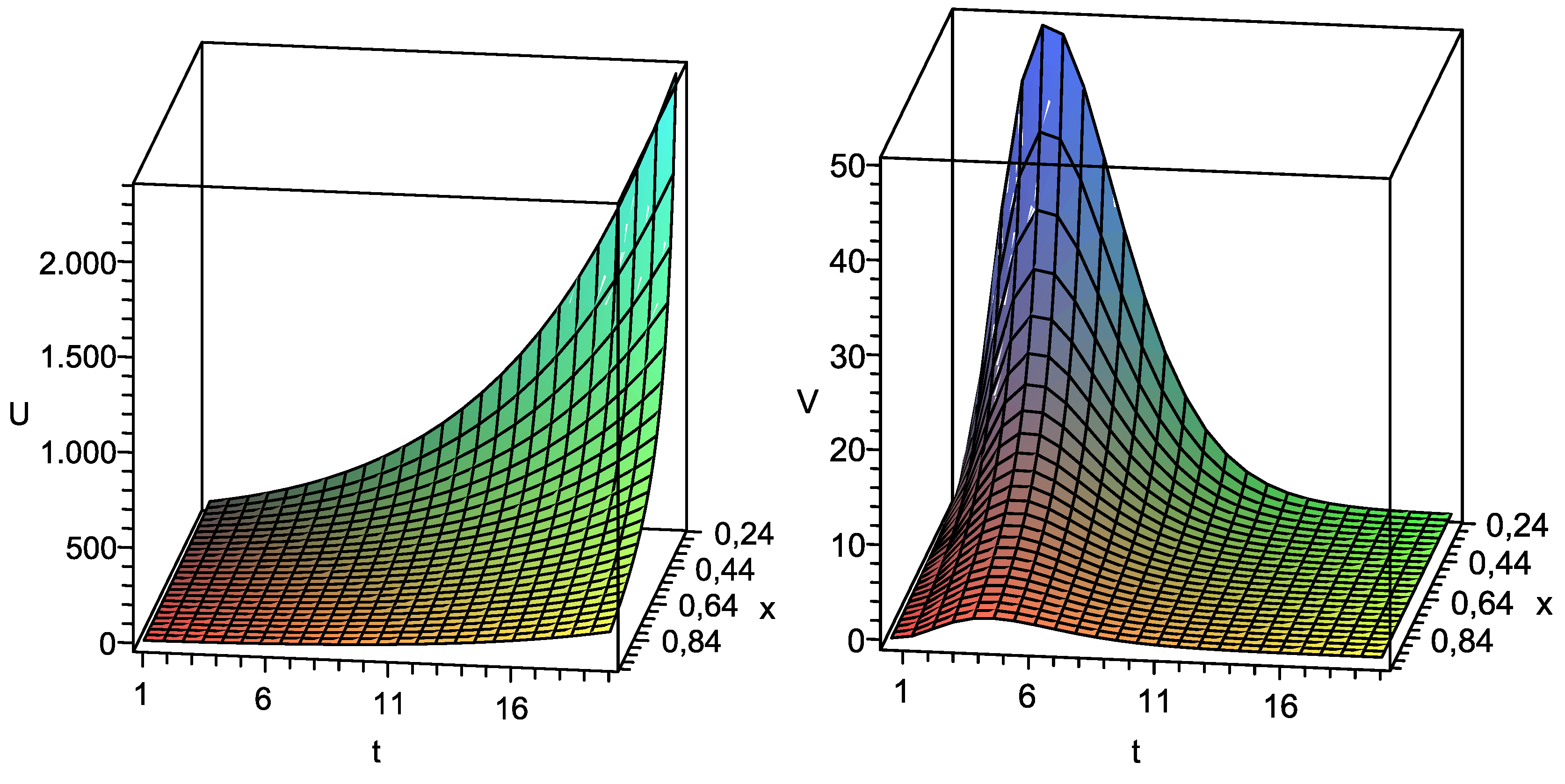
Thus, the species U in system (51) is prey and described by the first equation, while the second equation describes the predator density V. It can be established that the components of solution (52) with correctly-specified parameters are bounded and nonnegative in the relevant domains. For instance, the components of solution (52) with $k<-\frac{1}{\gamma }$ (otherwise $d_0<0$) are bounded and nonnegative in the domain $\left\{(t,x)\in \left[\frac{1}{6d_0},t_0\right]\times [x_0,1]\right\},$ where $t_0>\frac{1}{6d_0}$ and $x_0>0$ are arbitrary constants. Such a solution is presented in Figure 1 ($t_0=20,x_0=0.25$). One notes that the highest concentration of preys (component U) mostly corresponds to the lowest concentration of predators (component V). It is plausible behaviour of the species.

Figure 1. Solution (52) of system (51) with ${\alpha }_1=0.1,{\alpha }_2=0.75,\beta =5,\gamma =2$, $k=-1$, $l=-3$ and $d_0=1/6.$

Let us consider the second possible type of interaction between two species, which can be described by system (46). Applying the transformation

$$U=e^{-{\alpha }_{1}t}u,V=e^{-{\alpha }_{2}t}v$$

(54)

to system (46), we obtain the DLV system

$$\begin{array}{c}{U}_t=U_{xx}+U\left(-{\alpha }_1+\beta e^{{\alpha }_{1}t}{t}^{k}U+e^{{\alpha }_{2}t}{t}^{l}V\right),\hfill \\ V_t=d_0{V}_{xx}+V\left(-{\alpha }_2+e^{{\alpha }_{1}t}{t}^{k}U+\gamma e^{{\alpha }_{2}t}{t}^{l}V\right),\hfill \end{array}$$

(55)

that can describe symbiosis of two populations of species provided the parameters ${\alpha }_1,{\alpha }_2,\beta$ and $\gamma$ are positive. Using (50) and (54), one can obtain the corresponding exact solution of system (55).

4. Conclusions

In this paper, Lie symmetries of the DLV system (2) with time-dependent coefficients are studied. First of all the system was transformed to the form (5) in order to reduce the number of arbitrary functions. The main result is presented in Theorem 3 giving the exhaustive lists (Table 1 and Table 2) of the systems admitting the nontrivial Lie symmetries. All possible Lie symmetries of system (5) with arbitrary d (constant and nonconstant) were identified and presented in Table 1, while the DLV systems with $d=1$ and the relevant Lie symmetries and presented in Table 2. We note that for the coupled DLV system of the form (5) with $d=1$ (Cases 1–4 of Table 2) Lie symmetry operators were found under the restriction $q^1{q}^2=0$ (see the general form (22) of the Lie symmetry operator).

Finally, we have applied the Lie symmetry operator to reduce the Lotka–Volterra system (46) to the ODE system and to find an interesting exact solution. The exact solution obtained can satisfy the typical requirements occurring in biologically motivated problems describing the interaction of prey–predator type between two species.

References

- Volterra, V. Variazioni e fluttuazioni del numero d’individui in specie animali conviventi. Mem. Acad. Lincei 1926, 2, 31–113. [Google Scholar]
- Britton, N.F. Essential Mathematical Biology; Springer: Berlin, Germany, 2003. [Google Scholar]
- Lotka, A.J. Undamped oscillations derived from the law of mass action. J. Am. Chem. Soc. 1920, 42, 1595–1599. [Google Scholar] [CrossRef]
- Murray, J.D. Mathematical Biology II; Springer: Berlin, Germany, 2003. [Google Scholar]
- Cherniha, R.; Davydovych, V. Nonlinear Reaction-Diffusion Systems—Conditional Symmetry, Exact Solutions and Their Applications in Biology; Lecture Notes in Mathematics; Springer: Berlin, Germany, 2017; ISBN 978-3-319-65465-2. [Google Scholar]
- Hou, X.; Leung, A.W. Traveling wave solutions for a competitive reaction diffusion system and their asymptotics. Nonlinear Anal. Real World Appl. 2008, 9, 2196–2213. [Google Scholar] [CrossRef]
- Leung, A.W.; Hou, X.; Feng, W. Traveling wave solutions for Lotka–Volterra system re-visited. Discret. Contin. Dyn. Syst. 2011, 15, 171–196. [Google Scholar] [CrossRef]
- Cherniha, R.; Dutka, V. A diffusive Lotka–Volterra system: Lie symmetries, exact and numerical solutions. Ukr. Math. J. 2004, 56, 1665–1675. [Google Scholar] [CrossRef]
- Rodrigo, M.; Mimura, M. Exact solutions of a competition-diffusion system. Hiroshima Math. J. 2000, 30, 257–270. [Google Scholar]
- Hung, L.-C. Exact traveling wave solutions for diffusive Lotka Volterra systems of two competing species. Jpn. J. Ind. Appl. Math. 2012, 29, 237–251. [Google Scholar] [CrossRef]
- Cherniha, R.; Davydovych, V. Conditional symmetries and exact solutions of the diffusive Lotka Volterra system. Math. Comput. Model. 2011, 54, 1238–1251. [Google Scholar] [CrossRef]
- Cherniha, R. Lie symmetries of nonlinear two-dimensional reaction-diffusion Systems. Rep. Math. Phys. 2000, 46, 63–76. [Google Scholar] [CrossRef]
- Hou, Z.; Lisena, B.; Pireddu, M.; Zanolin, F. Lotka–Volterra and Related Systems: Recent Developments in Population Dynamics; Walter de Gruyter: Berlin, Germany, 2013; ISBN 978-3-11-026951-2. [Google Scholar]
- Bao, X.X.; Li, W.T.; Wang, Z.C. Time periodic traveling curved fronts in the periodic Lotka–Volterra competition-diffusion system. J. Dyn. Differ. Equ. 2017, 29, 981–1016. [Google Scholar] [CrossRef]
- Hetzer, G.; Shen, W. Convergence in almost periodic competition diffusion systems. J. Math. Anal. Appl. 2001, 262, 307–338. [Google Scholar] [CrossRef]
- Hutson, V.; Mischaikow, K.; Poláčik, P. The evolution of dispersal rates in a heterogeneous time-periodic environment. J. Math. Biol. 2001, 43, 501–533. [Google Scholar] [CrossRef] [PubMed]
- Struk, O.O.; Tkachenko, V.I. On impulsive Lotka–Volterra systems with diffusion. Ukr. Math. J. 2002, 54, 629–646. [Google Scholar] [CrossRef]
- Ovsiannikov, L.V. The Group Analysis of Differential Equations; Academic: New York, NY, USA, 1982. [Google Scholar]
- Ovsiannikov, L.V. Group relations of the equation of non-linear heat conductivity. Dokl. Akad. Nauk SSSR 1959, 125, 125492–125495. [Google Scholar]
- Zhdanov, R.Z.; Lahno, V.I. Group classification of heat conductivity equations with a nonlinear source. J. Phys. A Math. Gen. 1999, 32, 7405. [Google Scholar] [CrossRef]
- Kingston, J.G. On point transformations of evolution equations. J. Phys. A Math. Gen. 1991, 24, L769–L774. [Google Scholar] [CrossRef]
- Kingston, J.G.; Sophocleous, C. On form-preserving point transformations of partial differential equations. J. Phys. A Math. Gen. 1998, 31, 1597–1619. [Google Scholar] [CrossRef]
- Gazeau, J.P.; Winternitz, P. Symmetries of variable coefficient Korteweg-de Vries equations. J. Math. Phys. 1992, 33, 4087–4102. [Google Scholar] [CrossRef]
- Cherniha, R.; Davydovych, V.; King, J.R. Lie symmetries of nonlinear parabolic-elliptic systems and their application to a tumour growth model. ArXiv, 2017; arXiv:1704.07696. [Google Scholar]
- Cherniha, R.; King, J.R. Non-linear reaction diffusion systems with variable diffusivities: Lie symmetries, ansatze and exact solutions. J. Math. Anal. Appl. 2005, 308, 11–35. [Google Scholar] [CrossRef]
- Cherniha, R.; Serov, M.; Rassokha, I. Lie symmetries and form preserving transformations of reaction-diffusion-convection equations. J. Math. Anal. Appl. 2008, 342, 1363–1379. [Google Scholar] [CrossRef]
- Vaneeva, O.O.; Popovych, R.O.; Sophocleous, C. Enhanced group analysis and exact solutions of variable coefficient semilinear diffusion equations with a power source. Acta Appl. Math. 2009, 106, 1–46. [Google Scholar] [CrossRef]
- Cherniha, R.; Serov, M.; Pliukhin, O. Nonlinear Reaction-Diffusion-Convection Equations: Lie and Conditional Symmetry, Exact Solutions and Their Applications; CRC Press: Boca Raton, FL, USA, 2018; ISBN 9781498776172. [Google Scholar]
- Arrigo, D.J. Symmetry Analysis of Differential Equations: An Introduction; John Wiley and Sons: Hoboken, NJ, USA, 2015; ISBN 9781118721445. [Google Scholar]
- Bluman, G.W.; Cheviakov, A.F.; Anco, S.C. Applications of Symmetry Methods to Partial Differential Equations; Springer: New York, NY, USA, 2010; ISBN 978-0-387-68028-6. [Google Scholar]
- Olver, P.J. Applications of Lie Groups to Differential Equations; Springer: Berlin, Germany, 1986; ISBN 978-1-4684-0274-2. [Google Scholar]
- Nie, L.; Teng, Z.; Hu, L.; Peng, J. Permanence and stability in non-autonomous predator-prey Lotka–Volterra systems with feedback controls. Comput. Math. Appl. 2009, 58, 436–448. [Google Scholar] [CrossRef]
© 2018 by the author. Licensee MDPI, Basel, Switzerland. This article is an open access article distributed under the terms and conditions of the Creative Commons Attribution (CC BY) license (http://creativecommons.org/licenses/by/4.0/).