K-Hyperline Clustering-Based Color Image Segmentation Robust to Illumination Changes

Abstract

Color image segmentation is very important in the field of image processing as it is commonly used for image semantic recognition, image searching, video surveillance or other applications. Although clustering algorithms have been successfully applied for image segmentation, conventional clustering algorithms such as K-means clustering algorithms are not sufficiently robust to illumination changes, which is common in real-world environments. Motivated by the observation that the RGB value distributions of the same color under different illuminations are located in an identical hyperline, we formulate color classification as a hyperline clustering problem. We then propose a K-hyperline clustering algorithm-based color image segmentation approach. Experiments on both synthetic and real images demonstrate the outstanding performance and robustness of the proposed algorithm as compared to existing clustering algorithms.

1. Introduction

Image segmentation, which partitions images into multiple regions with similar characteristics, is commonly used for image analysis and understanding. Simultaneously, it is also a fundamental step for further image understanding [1] and directly affects the accuracy of many computer vision applications [2], such as object detection [3], object tracking [4,5] and image retrieval [6]. In general, existing color image segmentation methods can be classified into five categories: thresholding, clustering, edge detection, region extraction and saliency detection [7]. These methods are mainly based on watershed transform or clustering procedures [8]. The former computes the spatial gradient of image luminance; however, the chromatic information is ignored [9]. The latter depends on the balance of the pixel color distribution [10].

The most popular clustering algorithm is K-means clustering, which is an exclusive clustering algorithm based on minimizing formal objective function [11]. Although K-means is widely used and studied, it is sensitive to outliers that lead to converge to local minima so that its accuracy is not perfect and may fail to represent the data [12]. In order to overcome the weaknesses of K-means clustering. Ahmed M N et al. [13] proposed Fuzzy C-Means (FCM), which allows a pixel belonging to a different cluster at multiple degrees of memberships and has been successfully applied to MR image segmentation. To further improve the noise immunity of FCM, Krinidis et al. [14] proposed the Fuzzy Local Information C-Means (FLICM) clustering algorithm, which incorporates the spatial and gray information in a fuzzy way. Although FLICM promotes noise immunity and is free of parameter selection, the calculation of the local information is time consuming and limits its application in high dimension data. To reduce the computational complexity and enhance the robustness to outlines, Lei et al. [15] introduced a Fast and Robust Fuzzy C-Means (FRFCM), which uses morphological reconstruction to smooth the image and employs a faster membership to calculate the distance between the pixels and cluster centers.

However, these local information-based clustering algorithms such as FLICM and FRFCM clustering are not robust to illumination changes, i.e., pixels with identical colors, but different illuminations may be segmented into different segments (sets of pixels), which limits their real-world applications. To handle the illumination changes in scenes, Li and Miao [16] employed a two-layer Gaussian mixture model to represent the different illumination backgrounds and segment the foreground image regions based on the learned model. Delibasis et al. [17] proposed a video segmentation robust to change in illumination based on different background models. Although these approaches achieve favorable performance on many video sequences, the supervised pre-learned background model limits their application in single image segmentation. Additionally, the distribution of color is not fully utilized.

Motivated by the observation that the RGB value distributions of the same kind of color, which is captured under different illuminations, are located in an identical hyperline, we employ hyperline clustering to perform unsupervised model-free color classification-based image segmentation such that it is robust to varying illuminations. Then, we propose a novel color classification-based image segmentation method using the multilayer K-hyperline clustering algorithm, which is capable of finding K partitions of the image data that converge to a global minimum. Finally, we conduct numerous experiments to verify the competitive result of the proposed approach.

The reminder of this paper is organized as follows. Section 2 presents the K-hyperline clustering method. Section 3 describes the proposed illumination-invariant color segmentation approach. Experiments on synthetic and color images from the Berkeley Segmentation Dataset (BSDS500) are carried out in Section 4. The conclusions and future work are presented in Section 5.

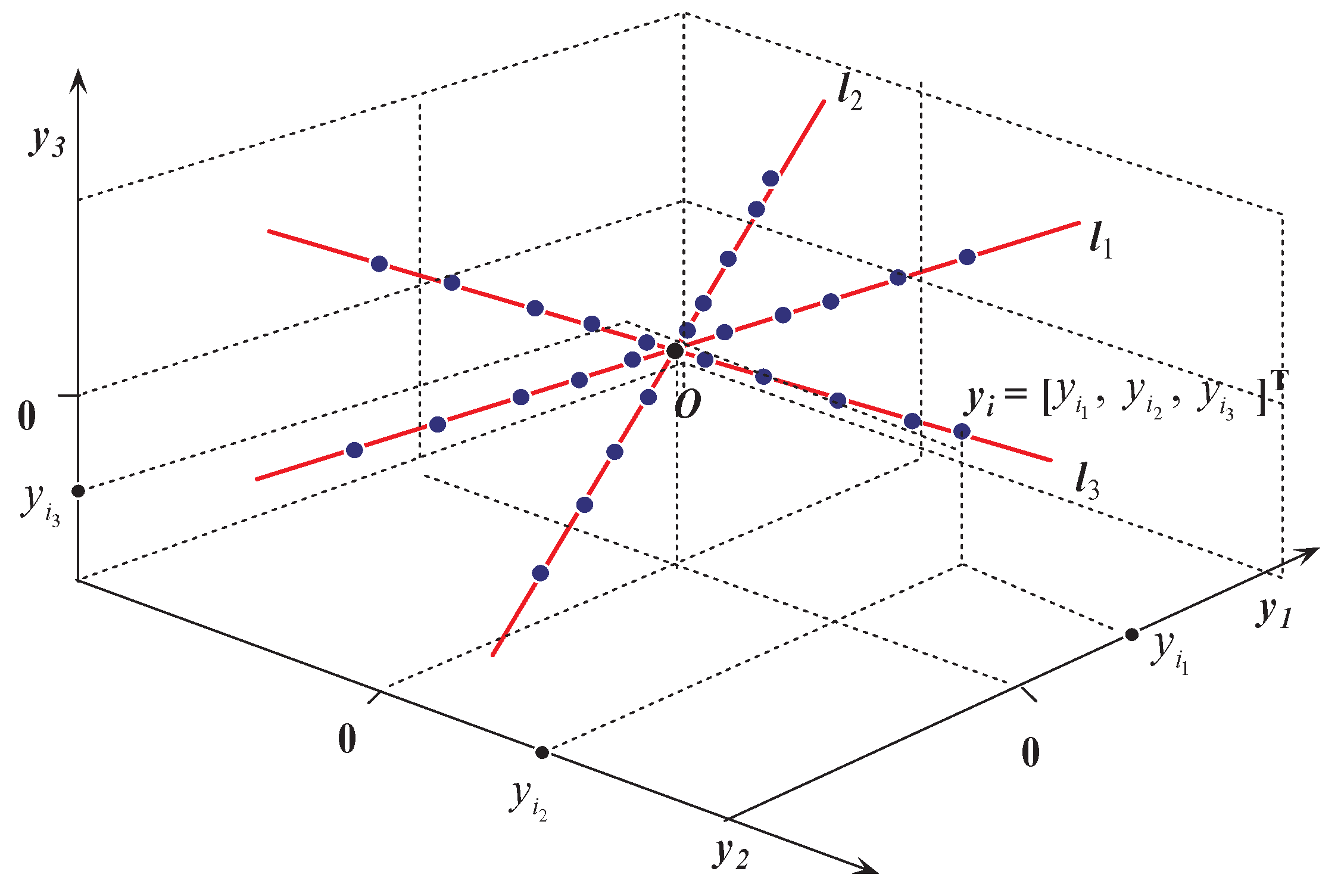
2. K-Hyperline Clustering

K-hyperline clustering is a special case of the general joint optimization problem of Sparse Component Analysis (SCA) [18]. The problem of SCA can be modeled as follows [19]:

$$\mathit{Y}=\mathit{AX}or\mathit{y}=\mathit{A}\mathit{x}$$

(1)

where matrix $\mathit{Y}=[{\mathit{y}}_1,\cdots ,{\mathit{y}}_T]\in {\mathbb{R}}^{m\times T}$ is an observed matrix, $\mathit{A}=[{\mathit{a}}_1,\cdots ,{\mathit{a}}_n]\in {\mathbb{R}}^{m\times n}$ is an unknown full row rank basis matrix and $\mathit{X}=[{\mathit{x}}_1,\cdots ,{\mathit{x}}_T]\in {\mathbb{R}}^{n\times T}$ is the matrix of sparse sources. When the sources $\mathit{X}$ are sparse enough to satisfy the disjoint orthogonality condition approximately, i.e., ${\mathit{x}}_i·{\mathit{x}}_j=0$, the model (1) can be rewritten as:

$$\mathit{y}=\mathit{A}\mathit{x}={\mathit{a}}_1·x_1+\cdots +{\mathit{a}}_n·x_n={\mathit{a}}_i·x_i$$

(2)

Equation (2) can be further simplified as:

$$\frac{y_1}{a_{i1}}=\frac{y_2}{a_{i2}}=\cdots =\frac{y_m}{a_{im}}=x_i$$

(3)

where ${\mathit{a}}_i={[a_{i1},\cdots ,a_{im}]}^T$. Since Equation (3) is a linear equation and all columns ${\mathit{a}}_1,\cdots ,{\mathit{a}}_m$ of $\mathit{A}$ are the hyperline directions of the observed data $\mathit{y}\left(t\right)$. In other words, finding the basis matrix $\mathit{A}$ can be considered as a hyperline clustering problem [20].

Given a set of observed data points ${\left\{{\mathit{y}}_i\right\}}_{i=1}^T$, which respectively are located on K-hyperlines $L\left({\mathit{l}}_k\right)$, where ${\mathit{l}}_k$ is the directional vector of the corresponding hyperline and $k=1,\cdots ,K$. K-Hyperline Clustering (K-HLC) aims to estimate K-hyperlines $L\left({\mathit{l}}_k\right)$ by identifying ${\mathit{l}}_k$, $k=1,\cdots ,K$, as shown in Figure 1.

Mathematically, K-HLC can be considered as the following optimization problem [21]:

$$\begin{array}{c}\hfill \underset{{\mathit{l}}_k,{\mathsf{\Omega }}_k,k=1,\cdots ,K}{min}J({\mathit{l}}_k,{\mathsf{\Omega }}_k,k=1,\cdots ,K)=\underset{{\mathit{l}}_k,{\mathsf{\Omega }}_k,k=1,\cdots ,K}{min}\sum _{i=1}^T\sum _{k=1}^K{d}^2({\mathit{y}}_i,{\mathit{l}}_k)\times I_{i\in {\mathsf{\Omega }}_k},\end{array}$$

(4)

where ${\mathit{l}}_k={[l_{k1},\cdots ,l_{km}]}^{\top }\in {\mathbb{R}}^m$ is the directional vector of hyperline $L\left({\mathit{l}}_k\right)$; the indicator function $I_{i\in {\mathsf{\Omega }}_k}$ is given by:

$$I_{i\in {\mathsf{\Omega }}_k}=\left\{\begin{array}{c}1,i\in {\mathsf{\Omega }}_k\hfill \\ 0,i\notin {\mathsf{\Omega }}_k\hfill \end{array}\right.$$

(5)

${\mathsf{\Omega }}_k$ denotes the k-th cluster set; the distance $d(\mathit{y},\mathit{l})$ from $\mathit{y}$ to $L\left({\mathit{l}}_k\right)$ is:

$$d(\mathit{y},\mathit{l})=\sqrt{\langle \mathit{y},\mathit{y}\rangle -\frac{\langle \mathit{y},\mathit{l}\rangle }{\langle \mathit{l},\mathit{l}\rangle }},$$

(6)

$\langle ·,·\rangle$ denotes the inner product.

Recently, He et al. [21] proposed a K-Hyperline Clustering (K-HLC) algorithm, which is not only robust to outliers, but can also detect the number of hidden hyperlines in an unsupervised manner. Furthermore, K-hyperline clustering is capable of avoiding local minima with a high probability by incorporating Fast Multilayer Initialization (FMI).

The first step of FMI is to segment the initial direction matrix ${\widehat{\mathit{L}}}^{\left(0\right)}=\mathit{Y}$ into M lower dimensional matrices ${\widehat{\mathit{L}}}_1^{\left(0\right)},\cdots ,{\widehat{\mathit{L}}}_M^{\left(0\right)}$, whose size are $m\times N_M$. Then, FMI constructs the initial direction matrix ${\mathit{L}}^{\left(0\right)}$ by selecting K possibly optimal columns from ${\widehat{\mathit{L}}}_i^{\left(0\right)}=[{\widehat{\mathit{l}}}_i^{\left(0\right)}\left(1\right),\cdots ,{\widehat{\mathit{l}}}_i^{\left(0\right)}(K+N_M)],i=1,\cdots ,M$. To select K optimal columns, all correlation coefficients $c({\mathit{l}}_i^{\left(0\right)}\left(k\right),\mathit{y}\left(t\right))={\left[{\mathit{l}}^{\left(0\right)}\right]}^T\left[\mathit{y}\left(t\right)\right]$ are computed, and the sample $\mathit{y}\left(t\right)$ is assigned to the k-th sets $\mathsf{\Omega }\left({\mathit{l}}_i^{\left(0\right)}\left(k\right)\right)$ if it satisfies $k=arg{max}_{j=1,\cdots ,K}\left\{\left|c\right({\mathit{l}}_i^{\left(0\right)}\left(j\right),\mathit{y}\left(t\right)|\right\}$. Finally, the $m\times K$ matrix ${\mathit{L}}^{\left(0\right)}$ is constructed by extracting K columns corresponding to the greatest number of set $\mathsf{\Omega }\left({\mathit{l}}_i^{\left(0\right)}\left(k\right)\right),k=1,\cdots ,K+N_M$. Through FMI, a high-dimensional hyperline matrix can be rapidly scanned, and efficient initialization can be achieved.

After initialization using FMI, K-HLC is implemented in a manner similar to that of K-means clustering in terms of the two steps: cluster assignment and cluster centroid update. In the cluster assignment step, observed data ${\left\{{\mathit{y}}_i\right\}}_{i=1}^T$ are assigned to ${\mathsf{\Omega }}_k$ by choosing k such that:

$$k=arg\underset{j=1,\cdots ,K}{min}{d}^2({\mathit{y}}_i,{\mathit{l}}_j)$$

(7)

In the second step, the cluster centroid is obtained by eigenvalue decomposition.

3. Color Image Segmentation Based on K-Hyperline Clustering

In this section, we illustrate the proposed color image segmentation method based on K-HLC in detail.

In the RGB color model, three primary colors (red, green and blue) are exploited together to produce an array of colors [22]. Thus, the RGB vector of a color pixel can be represented by:

$$\mathit{y}={[r,g,b]}^{\top }.$$

When the illumination changes, a simple and effective diagonal model, which maps colors under some reference illumination o to their corresponding color under another illumination u, is given by [23]:

$$\left(\begin{array}{c}{R}_o\\ G_o\\ B_o\end{array}\right)=\left(\begin{array}{ccc}{a}_1& 0& 0\\ 0& a_2& 0\\ 0& 0& a_3\end{array}\right)\left(\begin{array}{c}{R}_u\\ G_u\\ B_u\end{array}\right)$$

(8)

Model (8) can be rewritten as:

$${\mathit{y}}_o=\mathit{A}{\mathit{y}}_u$$

(9)

This model is similar to Model (1); thus, we employ K-HLC to solve the problem of illumination change.

To illustrate illumination changes, we generate a color grid with three primary colors—red (${[255,0,0]}^{\top }$) green (${[0,255,0]}^{\top }$) blue (${[0,0,255]}^{\top }$)—and three secondary colors—yellow (${[255,255,0]}^{\top }$) magenta (${[255,0,255]}^{\top }$) cyan (${[0,255,255]}^{\top }$)—under eight different illuminations, where we change their RGB values through reducing illumination using Photoshop software. The color grid image is shown in Figure 2a. Figure 2b shows that the pixel sequence ${\left\{{\mathit{y}}_{\mathit{i}}\right\}}_{i=1}^T$ of a color, for all illuminations on the color grid, is located on the same line, where:

$${\mathit{y}}_i={[r_i,g_i,b_i]}^{\top },$$

$i=1,\cdots ,T$ and T is the total number of image pixels. In other words, the pixels of the original images and their corresponding varied illumination ones are located on the same line. In detail, it is obvious that six hyperlines (straight lines for 3D space) corresponding to six colors are located in six direction for the linear distribution of different illumination. The normalized directional vectors are ${[1,0,0]}^{\top }$ (red color), ${[0,1,0]}^{\top }$ (green color), ${[0,0,1]}^{\top }$ (blue color), ${[\frac{1}{\sqrt[]{2}},\frac{1}{\sqrt[]{2}},0]}^{\top }$ (yellow color), ${[\frac{1}{\sqrt[]{2}},0,\frac{1}{\sqrt[]{2}}]}^{\top }$ (magenta color) and ${[0,\frac{1}{\sqrt[]{2}},\frac{1}{\sqrt[]{2}}]}^{\top }$ (cyan color), respectively. Thus, the color classification can be formulated as the hyperline clustering problem. Moreover, to suppress the outliers and obtain good performance against spots, we normalize ${\mathit{y}}_i$ such that $∥{\mathit{y}}_i∥=1$ and initialize the hyperlines $L\left({\mathit{l}}_k\right)$ using Fast Multilayer Initialization (FMI).

The proposed algorithm is summarized in Algorithm 1.

Algorithm 1: Color image segmentation based on K-HLC.

Input: Observed data ${\left\{{\mathit{y}}_i\right\}}_{i=1}^T$ and cluster number K.

1: Initialize the direction of hyperline ${\mathit{L}}^{\left(0\right)}=[{\mathit{l}}_1^{\left(0\right)},\cdots ,{\mathit{l}}_K^{\left(0\right)}]$ using FMI and the number of iterations $iter=0$. 2: Normalize $\left\{{\mathit{y}}_i\right\}$ such that $∥{\mathit{y}}_i∥=1$, $i=1,\cdots ,T$. 3: while$∥{\mathit{L}}^{\left(iter\right)}-{\mathit{L}}^{(iter-1)}∥<\epsilon$and$iter<num\_iter$ * do 4:  Assign data ${\left\{{\mathit{y}}_i\right\}}_{i=1}^T$ to K different clustering sets ${\mathsf{\Omega }}_k$, $k=1,\cdots ,K$. Data index $i\in {\mathsf{\Omega }}_k$ if and only if it satisfies $k=\mathit{a}rgmi{n}_{i=1,\cdots ,K}\left\{d^2(\mathit{y},{\mathit{l}}_i)\right\}$. 5:  Obtain a set of submatrices ${\mathit{Y}}_k=[{\mathit{y}}_1^k,\cdots ,{\mathit{y}}_{{\tilde{T}}_k}^k]$, where ${\tilde{T}}_k$ data ${\mathit{y}}_1^k,\cdots ,{\mathit{y}}_{{\tilde{T}}_k}^k$ are assigned to ${\mathsf{\Omega }}_k$. 6:  Compute the first eigenvector ${\mathit{u}}_{1k}$ of each matrix ${\mathit{Y}}_k·{\left({\mathit{Y}}_k\right)}^{\top }/$T, $k=1,\cdots ,K$. 7:  Update direction vectors ${\mathit{l}}_k$ using ${\mathit{u}}_{1k}$, $k=1,\cdots ,K$. 8:  $iter=iter+1$. 9: end while

Output: Clustering data ${\mathit{Y}}_k$, $k=1,\cdots ,K$.

* Usually, we can set $num\_iter=500$ and $\epsilon =0.05$.

4. Experimental Results and Discussion

We conducted numerical experiments to evaluate the performance of the proposed algorithm and performed comparisons with some existing methods. All experiments were tested in MATLAB R2015b, running on a Lenovo laptop with Intel I7 CPU 3.4 GHz and 8 GB RAM under Windows 7 Professional. First, we compared the proposed method with other algorithms in different color spaces. Second, we tested the synthetic images with different levels of illuminations. Third, we tested the method on images from the standard Berkeley Segmentation Dataset (BSDS500) [24]. The popular clustering segmentation methods: K-means, FCM, FILCM and FRFCM were employed in these for comparison, since the related codes are publicly accessible. The parameters of FILCM and FRFCM were selected following the suggestion of the authors. Besides, for a fair comparison, we set the same cluster number of all comparative approaches according to the ground truth without taking into account the spatial adjacency of pixels or the smoothness of segmentation boundaries. To evaluate the segmentation results quantitatively, we use Segmentation Accuracy (SA) as the performance measure, which is defined as follows [25]:

$$SA=\frac{\mathrm{Number}\mathrm{of}\mathrm{correctly}-\mathrm{classified}\mathrm{pixels}}{\mathrm{Total}\mathrm{number}\mathrm{of}\mathrm{pixels}}$$

(10)

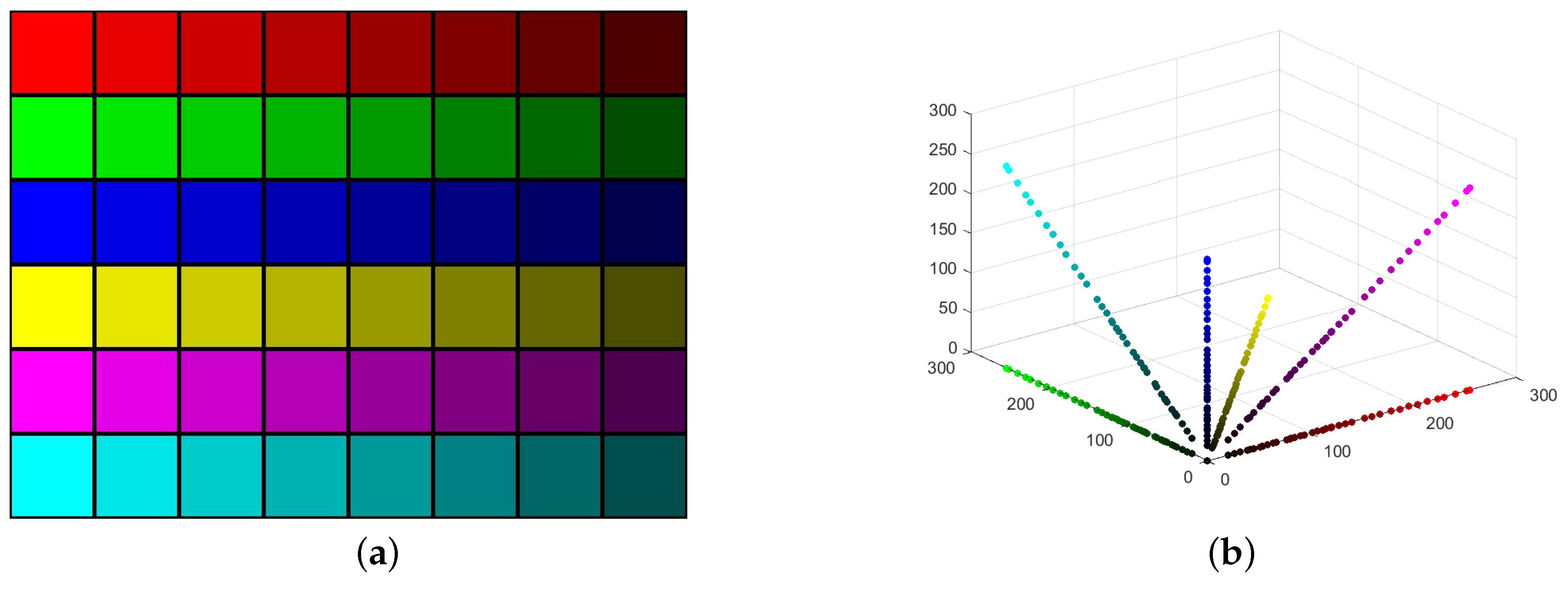
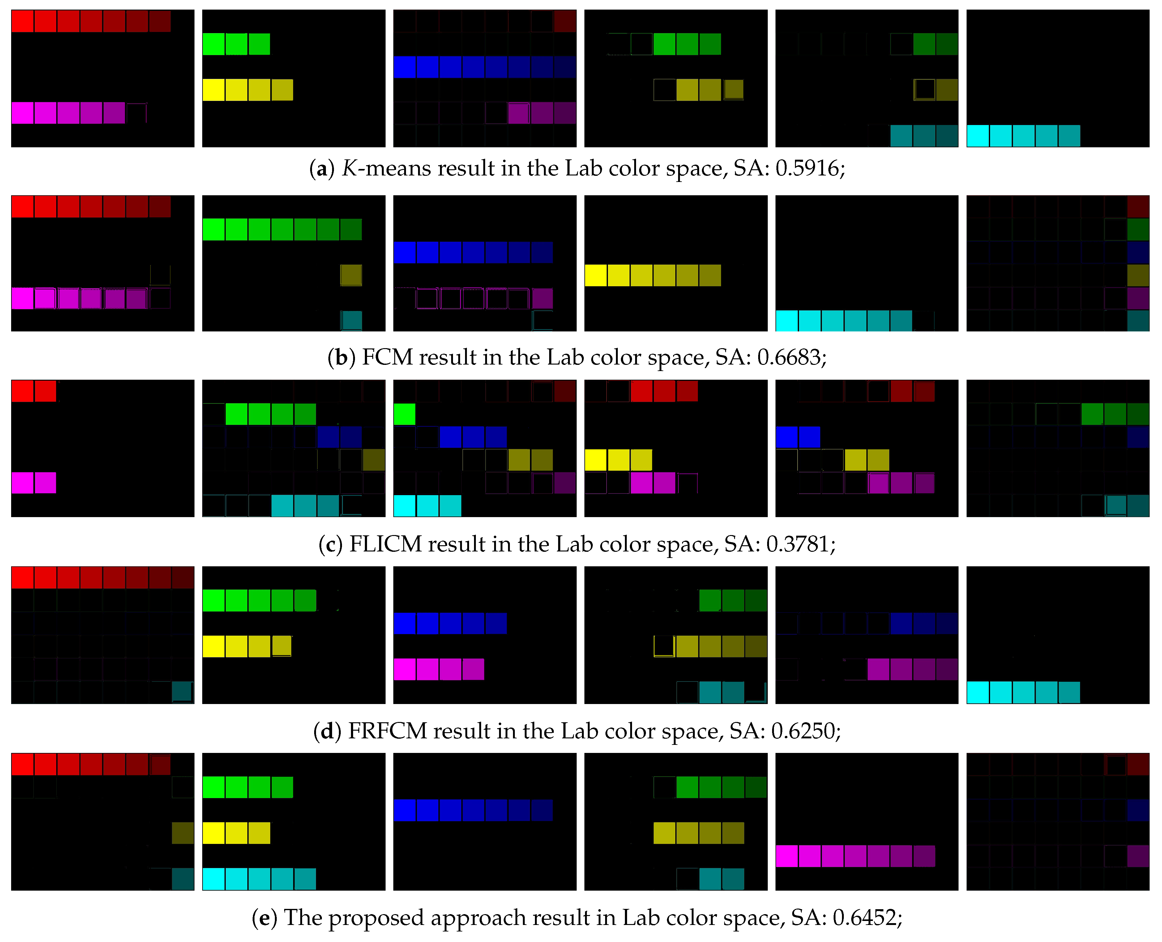
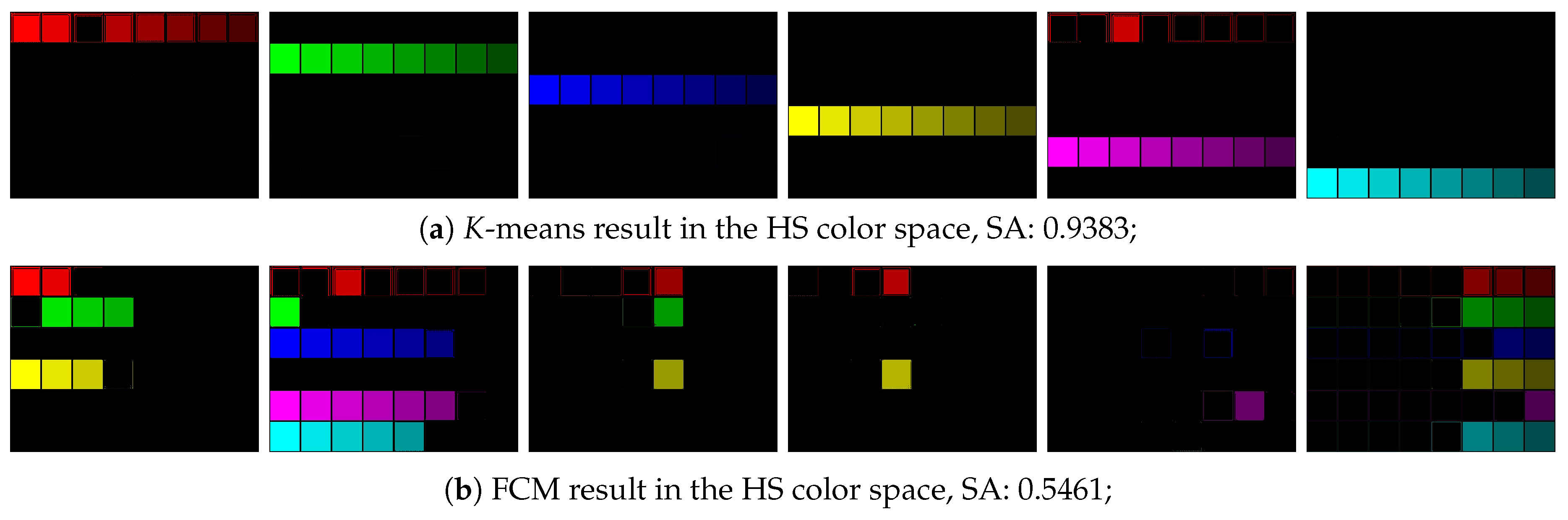
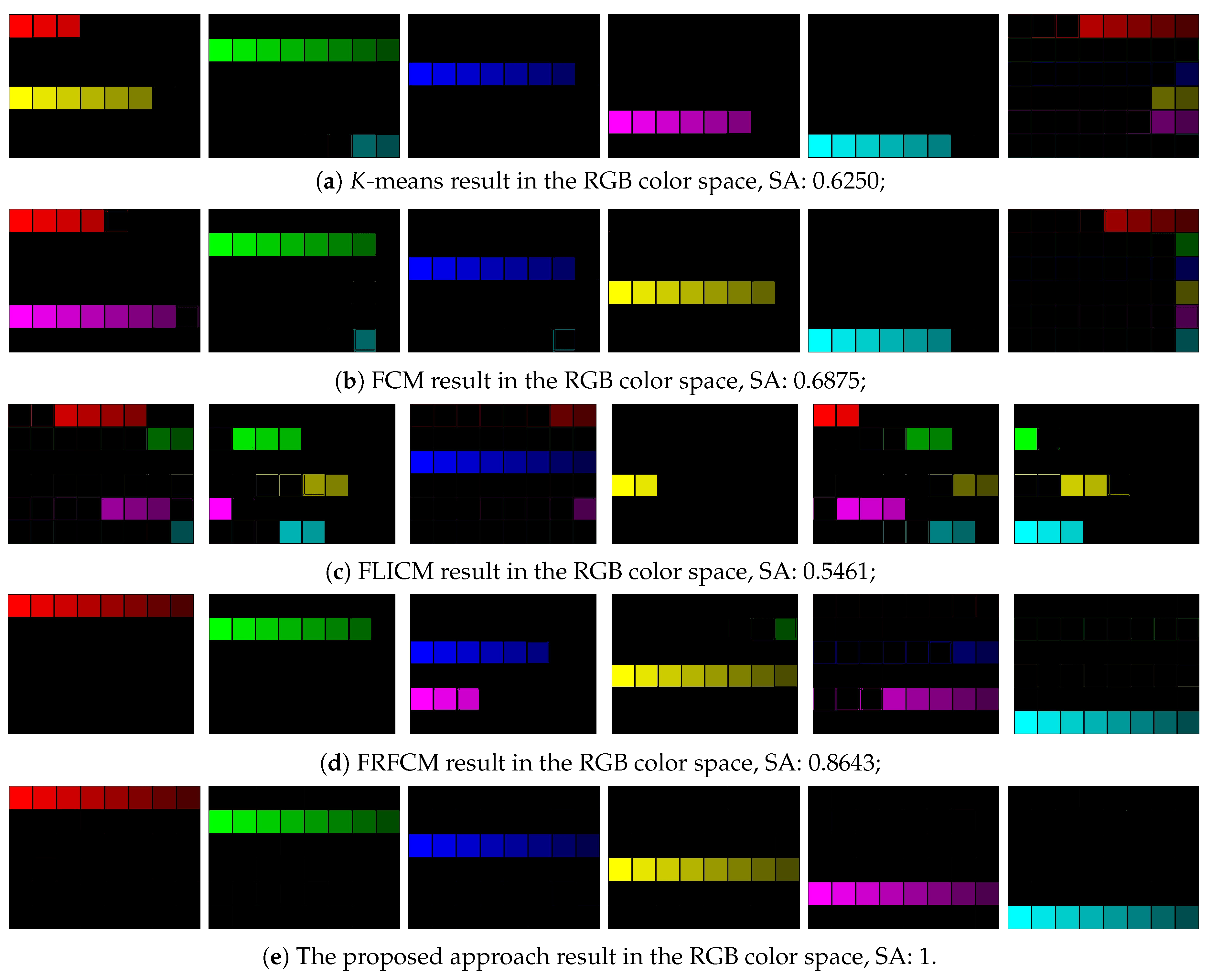
4.1. Results of Different Color Spaces

Besides widely used RGB color space, many color models, like HSL (Hue, Saturation, Lightness), HSV (Hue, Saturation, Value) and CIE-Lab, have been proposed to align with the human color vision system [25]. To demonstrate the superiority of the proposed method, we performed numerical experiments in different color spaces using Figure 2a. It is worth mentioning that we set the same RGB values of each grid. However, the marginal RGB value of each grid was different from the central one. This can be attributed to normalized function of MATLAB and is more challenging for a comparative algorithm. For the Lab color space, we utilized the MATLAB function “applycform” to convert the RGB value into the Lab color space. For HSL and HSV color spaces, to eliminate the effect of illuminations, we performed clustering procedures in the HS (Hue + Saturation) space. Since there are six colors in the color grid image, we set $K=6$ in the experiment.

In Figure 3, we show the results of different clustering algorithms in Lab color spaces. The SA are reported below each segmentation result. From the reported SA, we can observe that FCM obtains the best segmentation result in the Lab color space. However, it tends to classify the lowest illumination as the same cluster, as shown in the last cluster of Figure 3b.

Figure 4 shows the results of the HS color space. Note that only the K-means and FCM are presented. The provided codes of both FLICM and FRFCM are designed in one or three dimensions. Although K-means performed better than FCM in the HS color space, there were still many spots in the results of K-means, as shown in the fifth cluster of Figure 4a.

Figure 5 shows that FRFCM obtained a better performance than FILCM due to its morphological reconstruction. However, it failed to cope with low illumination. Among all of them, the proposed K-HLC-based method gave the most accurate segmentation and obtained the highest SA value of one in the RGB color space. This can be attributed to the linear distribution of the color grid image, as shown in Figure 2.

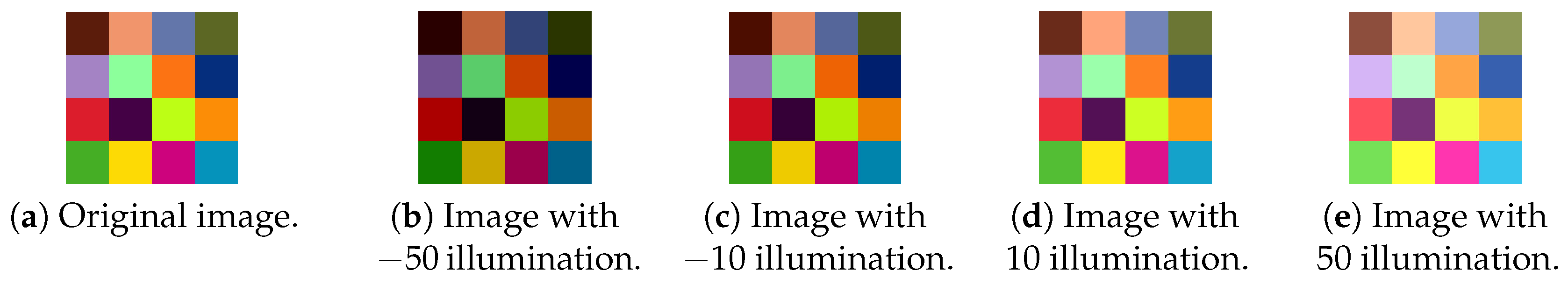
4.2. Results of Synthetic Color Images

In the this test, we generated a set of synthetic color images, whose levels of illuminations varied from $-50$% to 50%, as shown in Figure 6. For a fair comparison, We applied the proposed algorithm and other algorithms to both the original and normalized images. From

Table 1. SA of comparative methods for synthetic images. The best result is shown in bold font.

Illumination Levels (%)	$-50$	$-40$	$-30$	$-20$	$-10$	10	20	30	40	50
K-means	0.18	0.31	0.50	0.62	0.81	0.81	0.62	0.50	0.31	0.18
K-means (norm)	0.25	0.37	0.56	0.68	0.81	0.81	0.81	0.50	0.31	0.25
FCM	0.25	0.37	0.56	0.81	0.87	0.93	0.81	0.56	0.31	0.25
FCM (norm)	0.06	0.06	0.12	0.12	0.18	0.18	0.12	0.12	0.12	0.06
FLICM	0.32	0.42	0.56	0.65	0.81	0.81	0.68	0.62	0.48	0.35
FRFCM	0.58	0.61	0.78	0.89	0.96	0.96	0.89	0.77	0.63	0.61
Our method	$\mathbf{0.93}$	$\mathbf{1}$	$\mathbf{1}$	$\mathbf{1}$	$\mathbf{1}$	$\mathbf{1}$	$\mathbf{1}$	$\mathbf{1}$	$\mathbf{0.93}$	$\mathbf{0.93}$

, we can see that as the illumination changes, the SA values of normalized FCM clustering decreased much faster than others. This can be attributed to the performance of FCM completely depending on the location of the cluster center. It is worth noting that our method could correctly segment all 16 colors when illuminations varied from $-40$% to 30%. However, other clustering methods failed to classify different color grids when they suffered illumination changes. As we can see, the proposed approach yielded the best results for all ten illumination levels.

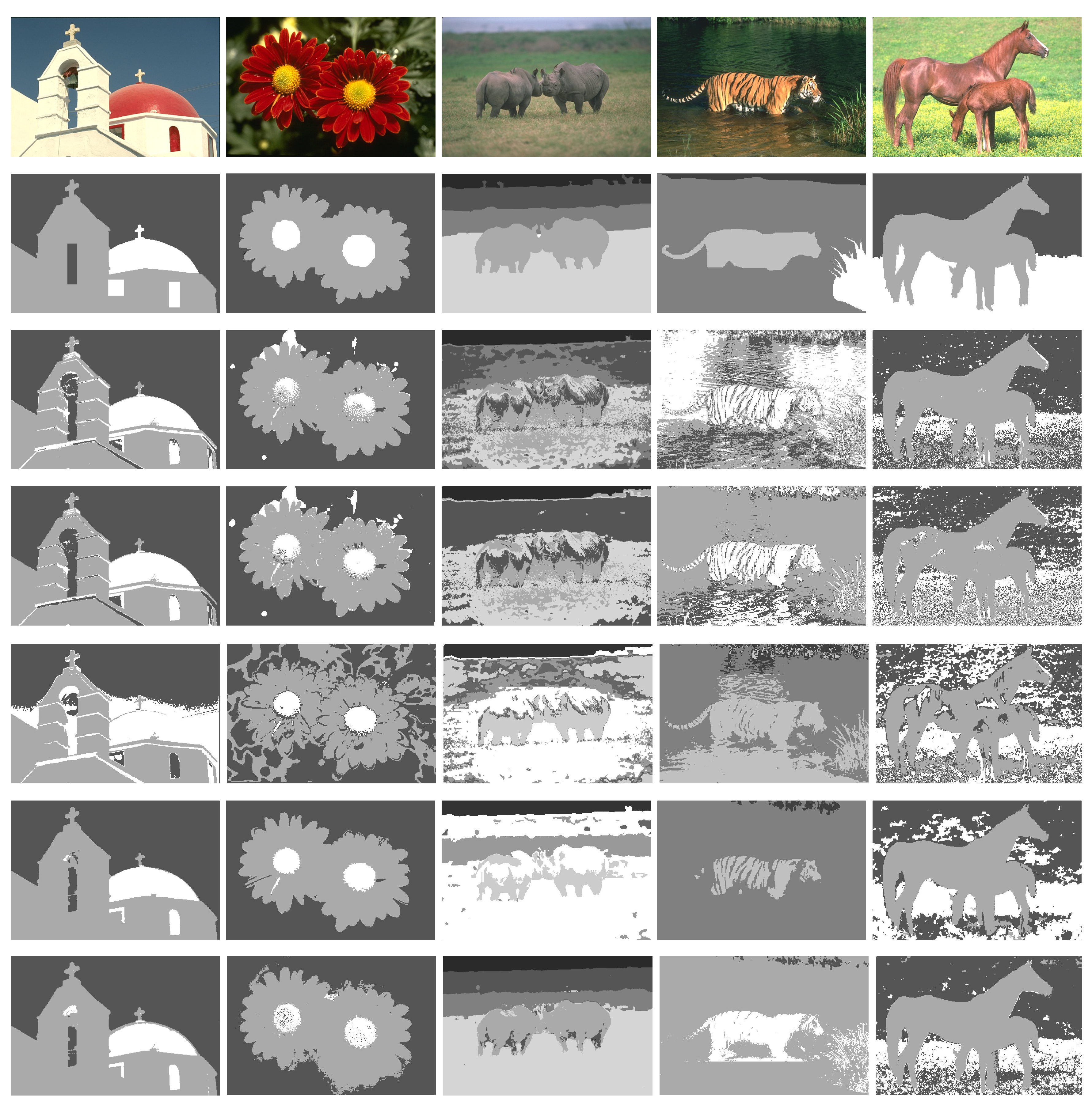
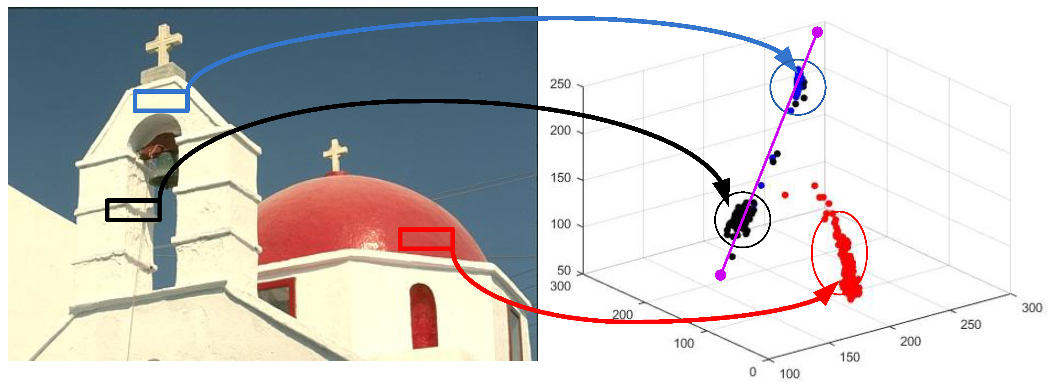
4.3. Results of Real- World Color Images

In the third test, we selected five real-world images from BSDS500 (church, flower, rhinoceros, tiger and horses). Note that the results are only associated with image color information without considering the spatial connection of pixels, and the segment number K was set according to the ground truths. The obtained segmentation SAs are shown in

Table 2. Comparison of SA for the BSDS500 images. The best result is shown in bold font.

Images (Name)	K-Means	FCM	FLICM	FRFCM	Ours
Church	0.9216	0.9246	0.8211	0.9730	$\mathbf{0.9795}$
Flower	0.8349	0.8457	0.7414	$\mathbf{0.9648}$	0.9387
Rhinoceros	0.5536	0.6105	0.6290	0.7266	$\mathbf{0.9348}$
Tiger	0.4180	0.6597	0.6461	0.8472	$\mathbf{0.8597}$
Horses	0.7425	0.7922	0.6643	0.8321	$\mathbf{0.9257}$

. From the table, we can observe that our method provided much more satisfactory results than K-means and FCM clustering, particularly for the rhinoceros and horses images where the illumination of the foreground was homogeneous with that of background. Although FRFCM obtained a higher SA than ours for the flower image, other images results demonstrated the superiority of our method. Figure 7 shows the segmentation results for the selected example. Visual inspection demonstrates that our method out-performed both conventional and state-of-the-art clustering methods. We attribute this to the illumination invariance of our approach, which helped to segment a connecting foreground. For example, the results of the horses image obtained by the other algorithms were not able to segment the background as well as ours. This can be attributed to the illumination immunity of the proposed method.

To illustrate our approach further, we performed a scatter plot of three different regions of the church image, as shown in Figure 8. The wall, shadow and dome regions are represented by blue, red and black arrow lines, respectively. As we can observe, the location of the black cluster is closer to that of the red cluster; thus, the K-means and FCM tended to classify these two regions as the same color because of the distance between the clusters. In contrast, our approach could detect the hyperline of the blue and black cluster (denoted by purple line); hence, the proposed approach was able to identify the same color in different illuminations and obtained color coherent segmentation.

5. Conclusions

In this study, we formulate color image classification as a hyperline clustering problem and then develop a novel and effective K-hyperline clustering-based color image segmentation approach, which is robust to illumination changes. Both qualitative and quantitative analyses demonstrate that the proposed algorithm outperforms the conventional K-means and FCM and more recent FLICM and FRFCM clustering approaches in different color spaces. The limitation of the proposed approach is that K-HLC has a run time that is twice that of the K-means clustering approach. Therefore, our future work will focus on the development of a more efficient hyperline clustering algorithm and also its application to illumination-invariant visual tracking and object detection.

References

1. Chen, J.; Zheng, H.; Lin, X.; Wu, Y.; Su, M. A novel image segmentation method based on fast density clustering algorithm. Eng. Appl. Artif. Intell. 2018, 73, 92–110. [Google Scholar] [CrossRef]
2. Gong, M.; Qian, Y.; Cheng, L. Integrated Foreground Segmentation and Boundary Matting for Live Videos. IEEE Trans. Image Process. 2015, 24, 1356–1370. [Google Scholar] [CrossRef] [PubMed]
3. Ren, S.; He, K.; Girshick, R.; Sun, J. Faster R-CNN: Towards Real-Time Object Detection with Region Proposal Networks. IEEE Trans. Pattern Anal. Mach. Intell. 2017, 39, 1137–1149. [Google Scholar] [CrossRef] [PubMed] [Green Version]
4. Čehovin, L.; Leonardis, A.; Kristan, M. Robust visual tracking using template anchors. In Proceedings of the 2016 IEEE Winter Conference on Applications of Computer Vision (WACV), Lake Placid, NY, USA, 7–10 March 2016; pp. 1–8. [Google Scholar] [CrossRef]
5. Mazzon, R.; Cavallaro, A. Multi-camera tracking using a Multi-Goal Social Force Model. Neurocomputing 2013, 100, 41–50. [Google Scholar] [CrossRef]
6. Jeong, J.; Won, I.; Yang, H.; Lee, B.; Jeong, D. Deformable Object Matching Algorithm Using Fast Agglomerative Binary Search Tree Clustering. Symmetry 2017, 9, 25. [Google Scholar] [CrossRef]
7. Li, F.; Qin, J. Robust fuzzy local information and LpLp-norm distance-based image segmentation method. IET Image Process. 2017, 11, 217–226. [Google Scholar] [CrossRef]
8. Yin, S.; Qian, Y.; Gong, M. Unsupervised Hierarchical Image Segmentation through Fuzzy Entropy Maximization. Pattern Recognit. 2017, 68, 245–259. [Google Scholar] [CrossRef]
9. He, L.; Li, Y.; Zhang, X.; Chen, C.; Zhu, L.; Leng, C. Incremental Spectral Clustering via Fastfood Features and Its Application to Stream Image Segmentation. Symmetry 2018, 10, 272. [Google Scholar] [CrossRef]
10. Moreno, R.; GranA, M.; Ramik, D.M.; Madani, K. Image segmentation on spherical coordinate representation of RGB colour space. Image Process. IET 2012, 6, 1275–1283. [Google Scholar] [CrossRef]
11. Kanungo, T.; Mount, D.M.; Netanyahu, N.S.; Piatko, C.D.; Silverman, R.; Wu, A.Y. An Efficient k-Means Clustering Algorithm: Analysis and Implementation. IEEE Trans. Pattern Anal. Mach. Intell. 2002, 24, 881–892. [Google Scholar] [CrossRef]
12. Nongmeikapam, K.; Kumar, W.K.; Singh, A.D. Fast and Automatically Adjustable GRBF Kernel Based Fuzzy C-Means for Cluster-wise Coloured Feature Extraction and Segmentation of MR Images. IET Image Process. 2018, 12, 513–524. [Google Scholar] [CrossRef]
13. Ahmed, M.N.; Yamany, S.M.; Mohamed, N.; Farag, A.A.; Moriarty, T. A modified fuzzy C-means algorithm for bias field estimation and segmentation of MRI data. IEEE Trans. Med. Imag. 2002, 21, 193–199. [Google Scholar] [CrossRef] [PubMed]
14. Krinidis, S.; Chatzis, V. A Robust Fuzzy Local Information C-Means Clustering Algorithm. IEEE Trans. Image Process. 2010, 19, 1328–1337. [Google Scholar] [CrossRef] [PubMed]
15. Lei, T.; Jia, X.; Zhang, Y.; He, L.; Meng, H.; Nandi, A.K. Significantly Fast and Robust Fuzzy C-Means Clustering Algorithm Based on Morphological Reconstruction and Membership Filtering. IEEE Trans. Fuzzy Syst. 2018, 26, 3027–3041. [Google Scholar] [CrossRef]
16. Li, J.; Miao, Z. Foreground segmentation for dynamic scenes with sudden illumination changes. Image Process. IET 2012, 6, 606–615. [Google Scholar] [CrossRef]
17. Delibasis, K.K.; Goudas, T.; Maglogiannis, I. A novel robust approach for handling illumination changes in video segmentation. Eng. Appl. Artif. Intell. 2016, 49, 43–60. [Google Scholar] [CrossRef]
18. Xie, K.; He, Z.; Cichocki, A.; Fang, X. Rate of Convergence of the FOCUSS Algorithm. IEEE Trans. Neural Netw. Learn. Syst. 2017, 28, 1276–1289. [Google Scholar] [CrossRef] [PubMed]
19. Xie, K.; He, Z.; Cichocki, A. Convergence analysis of the FOCUSS algorithm. IEEE Trans. Neural Netw. Learn. Syst. 2017, 26, 601–613. [Google Scholar] [CrossRef] [PubMed]
20. Bofill, P.; Zibulevsky, M. Underdetermined blind source separation using sparse representations. Signal Process. 2001, 81, 2353–2362. [Google Scholar] [CrossRef] [Green Version]
21. He, Z.; Cichocki, A.; Li, Y.; Xie, S.; Sanei, S. K-hyperline clustering learning for sparse component analysis. Signal Process. 2009, 89, 1011–1022. [Google Scholar] [CrossRef] [Green Version]
22. Swain, M.J.; Ballard, D.H. Color indexing. Int. J. Comput. Vision 1991, 7, 11–32. [Google Scholar] [CrossRef]
23. Finlayson, G.D.; Drew, M.S.; Funt, B.V. Diagonal transforms suffice for color constancy. In Proceedings of the International Conference on Computer Vision, Berlin, Germany, 11–14 May 1993; pp. 164–171. [Google Scholar]
24. Arbeláez, P.; Maire, M.; Fowlkes, C.; Malik, J. Contour detection and hierarchical image segmentation. IEEE Trans. Pattern Anal. Mach. Intell. 2011, 33, 898–916. [Google Scholar] [CrossRef] [PubMed]
25. Smith, A.R. Color gamut transform pairs. ACM Siggraph Comput. Graph. 1978, 12, 12–19. [Google Scholar] [CrossRef]
Figure 1. Hyperline clustering, observed data points y i i = 1 T (blue points) and hidden hyperlines (red lines).
Symmetry 10 00610 g001
Figure 2. (a) Color grid of six different colors under varying illuminations. (b) Scatter plot of the color grid in (a), where the colors of scatter points correspond to those of image pixels.
Symmetry 10 00610 g002
Figure 3. Experimental results in the Lab color space. SA, Segmentation Accuracy; FLICM, Fuzzy Local Information C-Means; FRFCM, Fast and Robust Fuzzy C-Means.
Symmetry 10 00610 g003
Figure 4. Experimental results in the HS color space.
Symmetry 10 00610 g004
Figure 5. Experimental results in the RGB color space.
Symmetry 10 00610 g005
Figure 6. Synthetic image, image with different level illuminations.
Symmetry 10 00610 g006
Figure 7. Color image segmentation of the BSDS500 images (church, flower, rhinoceros, tiger and horses). The first row shows the original images. The second row shows the ground truths. The third row shows the results of K-means clustering. The fourth row shows the result of FCM clustering. The fifth row shows the results of FLICM. The sixth row shows the results of FRFCM. The seventh row shows the results of our method.
Symmetry 10 00610 g007
Figure 8. Scatter plot of three different regions of the church image. The wall, shadow and dome regions are represented by blue, red and black arrow lines, respectively.
Symmetry 10 00610 g008