Abstract
Existing variance control charts are designed under the assumptions that no uncertain, fuzzy and imprecise observations or parameters are in the population or the sample. Neutrosophic statistics, which is the extension of classical statistics, has been widely used when there is uncertainty in the data. In this paper, we will originally design control chart under the neutrosophic interval methods. The complete structure of the neutrosophic control chart will be given. The necessary measures of neutrosophic will be given. The neutrosophic coefficient of control chart will be determined through the neutrosophic algorithm. Some tables are given for practical use. The efficiency of the proposed control chart is shown over the control chart designed under the classical statistics in neutrosophic average run length (NARL). A real example is also added to illustrate the proposed control chart. From the comparison in the simulation study and case study, it is concluded that the proposed control chart performs better than the existing control chart under uncertainty.
1. Introduction
In this modern era, the customers demand high-quality products or services to fulfill their needs. High quality in a product can be only achieved if the manufacturing process meets the given specifications limits. To the manufacturer to produce the defect-free product, the variation in the process should be controlled. Generally, the manufacturing process moves away from control limits due to two types of variation, which are called the natural variation and special variation. Therefore, to produce the high-quality product that meets the given standard the elimination of variation is necessary. The control chart is one of the important tools that have been widely used in the industry for the monitoring of the process. The control chart immediately informs the engineers if any problem occurs that can shift the process from its target. According to Abbas et al. [1], “Dispersion charts are used to monitor within samples variability while location charts are used to monitor between samples variability. So, it is preferable to monitor the process dispersion before the location of the process”. Among the control chart, the Shewhart [2] control chart is easy to apply in the industry. The Shewhart [2] control chart has an upper control limit (UCL), a lower control limit (LCL) and central limit (CL). There are many other signals, such as two points out of three points to be out-of-control and four points out of five points to be out-of-control, which determine if the process is “out-of-control” or not. A process is declared to be out-of-control if the plotting statistic lies beyond the UCL or LCL. But, the first point to be out-of-control follows the geometric distribution. This criterion has been widely used to find the average run length to assess the performance of the control chart. The control charts under classical statistics have been studied by many authors, for example, Khoo [3] proposed control chart for the double sampling. Zhang et al. [4] presented the design of control chart. Khoo [5] studied the modified form of dispersion chart. Lee et al. [6] worked for this chart under the interval sampling. Riaz [7] presented a dispersion chart based on Interquartile range. Guo and Wang [8] studied the dispersion chart when the variance is estimated. Some details on the dispersion control chart can be seen in references [1,9].
The fuzzy approach has been widely applied in the uncertainty environment, see Zadeh [10]. According to Senturk and Erginel [11] “observations include human judgments, and evaluations and decisions, a continuous random variable of a production process should include the variability caused by human subjectivity or measurement devices, or environmental conditions. These variability causes create vagueness in the measurement system”. Therefore, the fuzzy control charts have been widely applied in a situation when there is uncertainty. Several authors worked on the designing of control chart using the fuzzy approach. The authors of [12,13] proposed fuzzy control charts for the Statistical Process Control (SPC) zone rules. Senturk and Erginel [11] proposed fuzzy dispersion control charts. Mojtaba et al. [14] proposed the fuzzy chart using triangle fuzzy random variable. Shu et al. [15] proposed the fuzzy chart using data-adoptability approach. Afshari and Gildeh [16] designed a fuzzy control chart using the multiple dependent state (MDS) sampling. Fadaei and Pooya [17] proposed the fuzzy U control chart. More detail on the control charts using the fuzzy approach can be seen in references [15,18].
The authors of [19] mentioned that fuzzy logic is the special case of the neutrosophic logic. Smarandache [20] introduced some basic work in the neutrosophic statistics. According to [20], the neutrosophic statistics can be applied when the observations or the parameters are imprecise, indeterminate and fuzzy. Recently, the authors of [21,22] worked on rock study issues using the neutrosophic statistics. References [23,24] introduced the neutrosophic sampling plan the first time.
A rich literature on control chart for the monitoring of the variation or shift in the dispersion parameter is available under classical statistics. For the monitoring of the dispersion parameter, the control chart has been widely used in the industry. The existing literature of control charts is designed under the assumption that there is no uncertainty, indeterminacy, imprecise and fuzzy observations/parameter in the data. In practice, due to the measurement process, it may not possible to record data having all observations determined. So, when the observations are imprecise and uncertain, the control charts under the classical statistics cannot be applied. The neutrosophic statistics, which is the generalization of the classical statistics, deal with the situations when the observations or parameters are fuzzy. The neutrosophic statistics is used when the population or the sample has some uncertain observations.
According to the best of our knowledge, there is no study on the design of control chart using the neutrosophic statistics. In this paper, our objective is to originally design a control chart under the neutrosophic interval methods. The efficiency of the proposed chart will be compared with the chart under the classical statistics in terms of neutrosophic average run length. The design of the proposed control chart is given in Section 2. In Section 3, the advantages of the proposed control chart are discussed. A case study is given in Section 4 and some concluding remarks are given in the last section.
2. Design of Proposed Control Chart
A random sample selected from such a population or the sample having indeterminacy in observations is called a neutrosophic random sample. Suppose a neutrosophic random number 1, 2, 3, …, , where is a determinate part and is an indeterminate part. Let ; represent the mean of population having indeterminate observations; where and are the means of determinate part and indeterminate parts, respectively and ; represents the neutrosophic population variance, where and are the variance of determinate part and indeterminate parts, respectively. Let ; and ; be the neutrosophic sample mean and neutrosophic variance of . More detail can be seen in [20]. In this section, we will propose the following control chart under the neutrosophic statistical interval method. The proposed chart emphasized that variable inspection (measuring the quality of interest) is used to monitor the variance of the process.
Step-1: Select a random sample of size from the production process and compute .
Step-2: Declare the process is in-control state if ; where and are neutrosophic interval control limits.
The neutrosophic control limits and are given by
where is a neutrosophic control chart coefficient and will be determined through the neutrosophic algorithm.
The proposed control chart under the neutrosophic statistical interval method is the generalization of control chart under the classical statistics. The proposed chart becomes the existing control chart under the classical statistics when . The probability that the process is declared to be out-of-control under the neutrosophic interval methods is derived as follows:
Note here that ; , follows the neutrosophic Chi-square ; distribution with neutrosophic degree of freedom ; when the process is in-control state. The hypothesis is that the process is in-control state at . Suppose be the neutrosophic distribution function of . Therefore, for the in-control state,
Similarly,
The probability of in-control process under the neutrosophic interval method is given by:
The average run length (ARL) under the classical statistics is an important measure used to assess the performance of the control chart. The ARL indicates that when, on average, the process will be out-of-control and when it is actually an in-control state. The neutrosophic average run length (NARL) under the neutrosophic interval method is defined by:
Now suppose that the variance of the process has shifted to new target value ;, where denotes the shift constant. The alternative hypothesis for this study is that the process has shifted to a new variance . Note here that ; , follows the neutrosophic Chi-square ; distribution with neutrosophic degree of freedom ; when the process is an out-of-control state.
The probability that the process is declared to be out-of-control for the shifted process under the neutrosophic interval methods is derived as follows
Therefore, for the out-of-control state at is given by
Similarly,
The probability of an out-of-control process at under the neutrosophic interval method is given by:
The NARL for the shifted process is given by:
Let denote the specified values of . The values of NARL for various subgroup size and shift are presented in Table 1, Table 2 and Table 3. In Table 1, the values of NARL are given when and = 300 and 370. In Table 2, the values of NARL are given when and = 300 and 370. In Table 3, the values of NARL are given when and = 300 and 370. From Table 1, Table 2 and Table 3, the following trends in NARL can be noted.

Table 1.
The neutrosophic plan parameters when and = 300,370.
Table 2.
The neutrosophic plan parameters when and = 300,370.
Table 3.
The neutrosophic plan parameters when and = 300,370.
- For the fixed values of and , the range in indeterminacy interval of NARL increases as decreases from 300 to 370.
- For the fixed values of and , the range in indeterminacy interval of NARL decreases as increases.
The following neutrosophic algorithm is applied to determine the indeterminacy interval of .
- Step-1:
- Specify the indeterminacy interval of and .
- Step-2:
- Determine the indeterminacy interval of such that .
- Step-3:
- Find indeterminacy interval of using selected in Step-2.
3. Comparison Studies
In this section, we will compare the efficiency of the proposed control chart under the neutrosophic interval method with control chart under the classical statistics.
3.1. Comparison by NARL
We will present the comparison in NARL when and = 300 in Table 4. According to the authors of [22], a method which provides the parameters in indeterminacy interval rather than the determined value under the uncertainty environment, is said to be more effective and adequate. From Table 4, it can be noted that the proposed control chart under the neutrosophic statistics has NARL in indeterminacy interval, while the existing chart under the classical statistics provides the determined value. For example, when = 1.1, the indeterminacy interval of the proposed chart is while ARL = 167 from the existing control chart. From the comparison, it can be concluded that the existing control chart cannot be applied when some observations/parameters are uncertain. Therefore, by following the theory proposed in [22], the proposed control chart is more effective and adequate than control chart under classical statistics.
Table 4.
Comparison when [4,6] and .
3.2. Comparison by Simulation
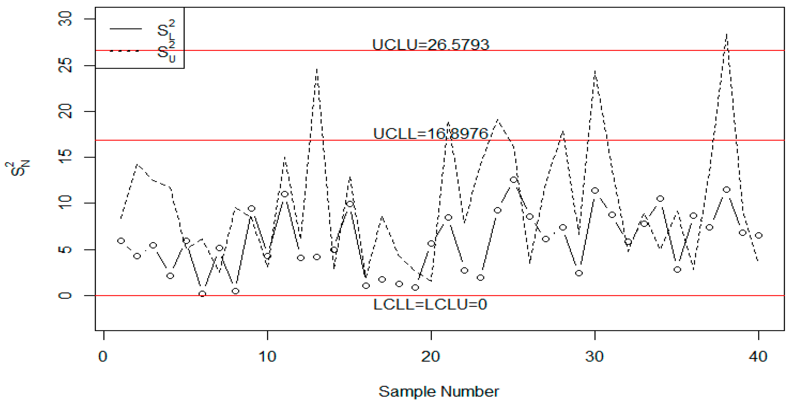
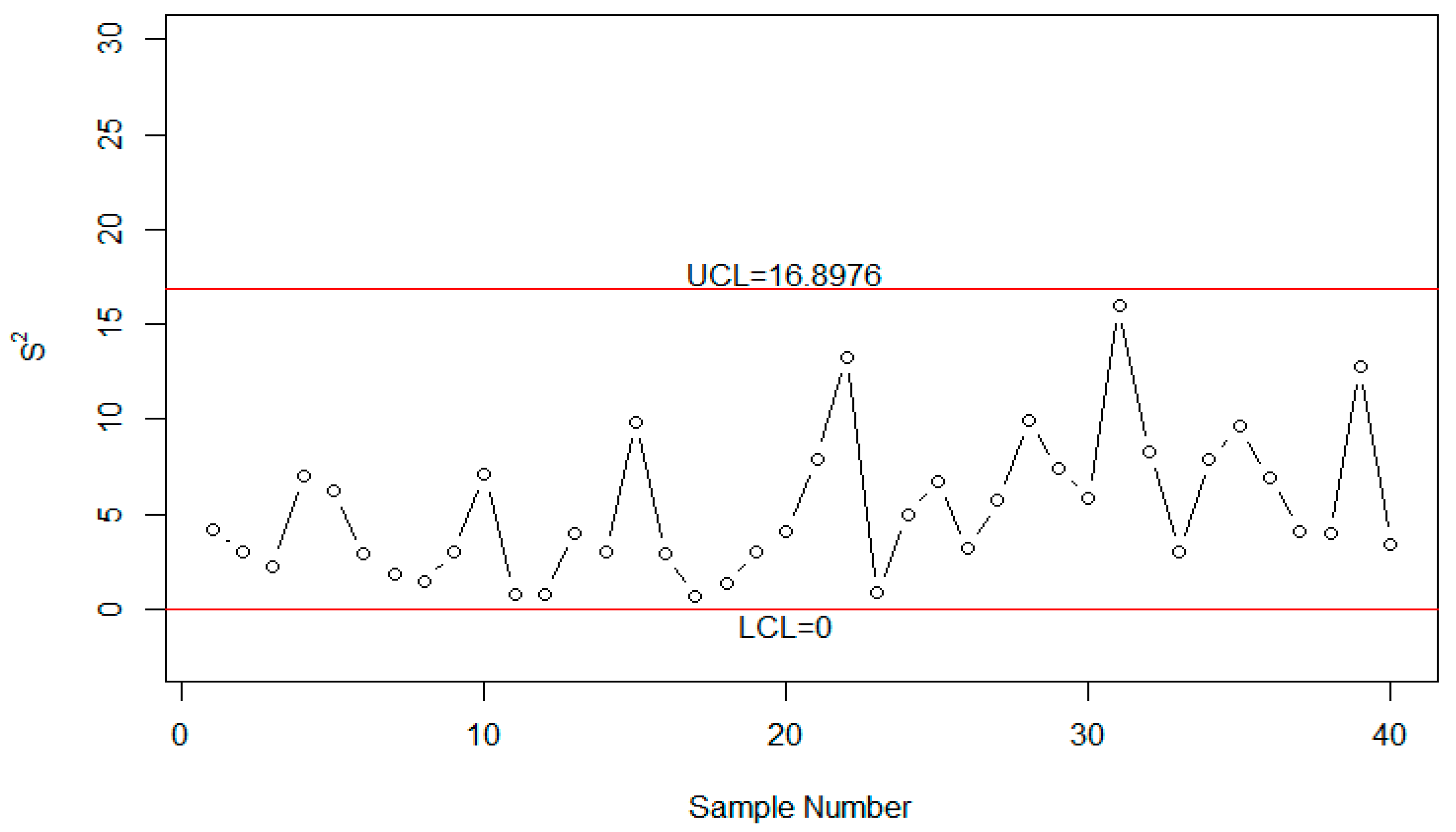
We now compare the efficiency of the proposed control with the control chart under the classical statistics by using the simulation data. The data is generated from the neutrosophic normal distribution with and neutrosophic variance . The first 20 neutrosophic observations are generated from the in-control process and next 20 neutrosophic observations from the shifted process with = 1.8. For the simulation study, let and = 370. We plotted the neutrosophic statistic on Figure 1. It is expected that the proposed chart should detect a shift in the indeterminacy interval . From Figure 1, it can be noted that the proposed plan detect a shift in the process at the 19th sample. The same values statistic under the classical statistic is plotted in Figure 2. Figure 2 indicates that the process is an in-control state. By comparing Figure 1 with Figure 2, it is concluded that the proposed control chart has the ability to detect a shift in the process. Also, the proposed control chart is more effective in the uncertainty environment.
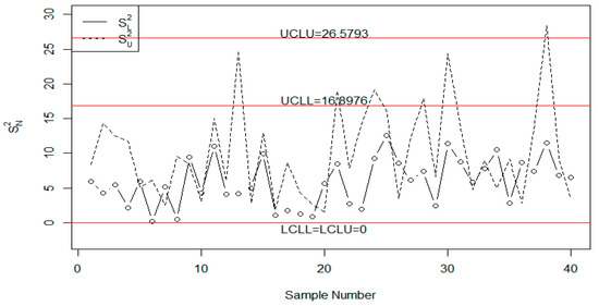
Figure 1.
The proposed chart under the neutrosophic interval statistical method.
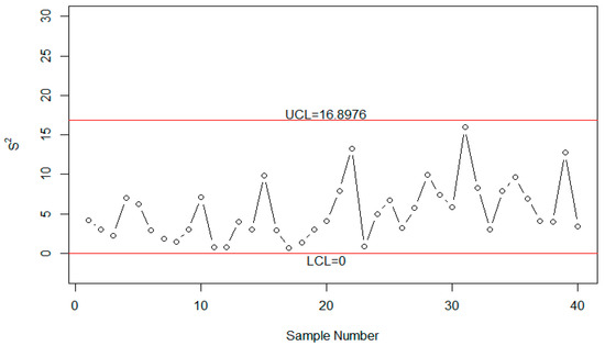
Figure 2.
The control chart under the classical statistics.
4. Case Study
The application of the proposed chart is given in the automobile industry. In this industry, the measurement of the inside diameter of engine piston rings is an important variable, see Montgomery [25]. Therefore, the monitoring of this variable is an important task in the automobile industry. The inside diameter is a continuous variable. Due to human subjectivity or measurement devices and environmental conditions, it is possible that some observations are uncertain. In this case, the control chart under classical statistics cannot be applied for the monitoring of the diameter. The data having some uncertain observations are reported in Table 5.
Table 5.
Real example data.
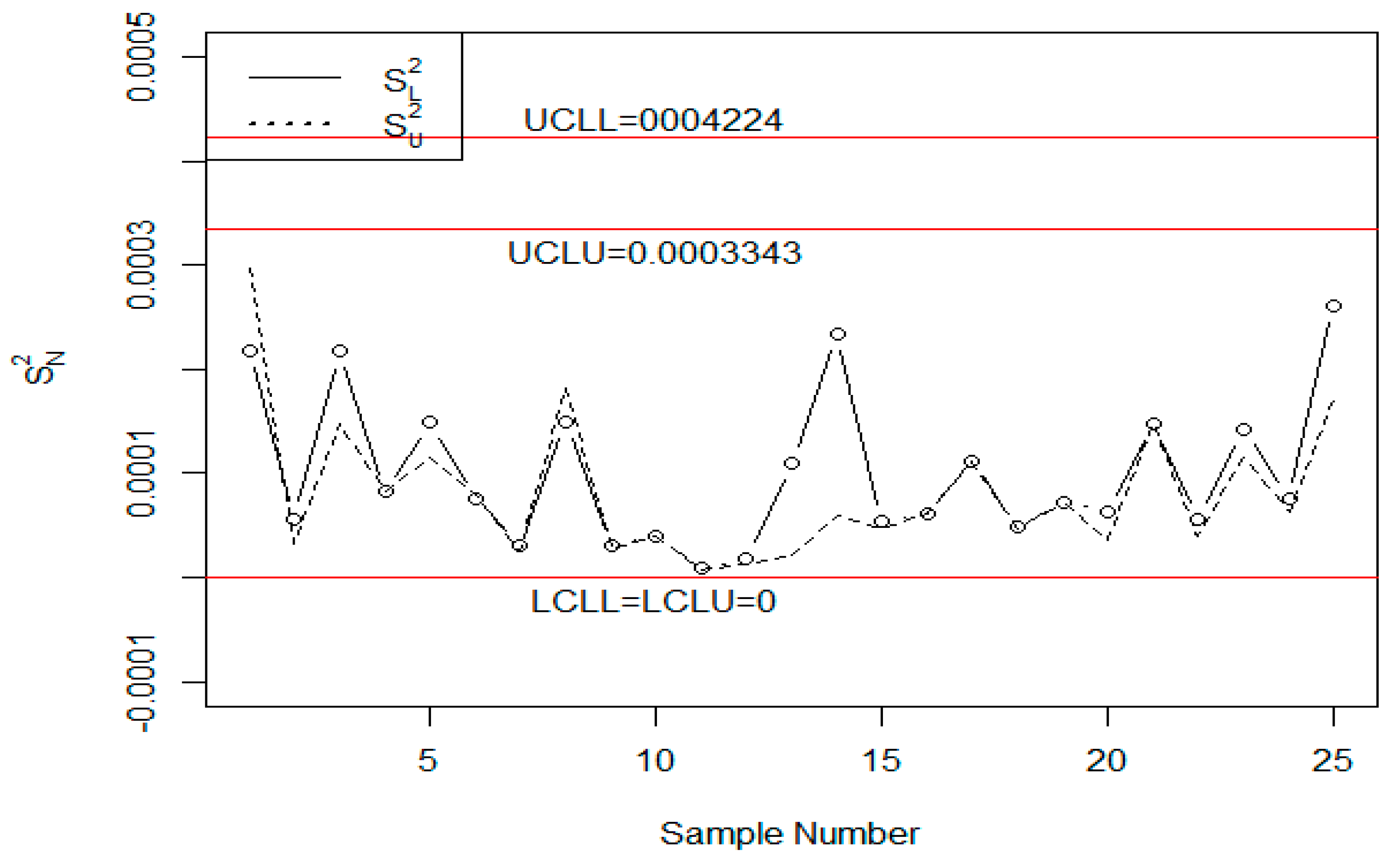
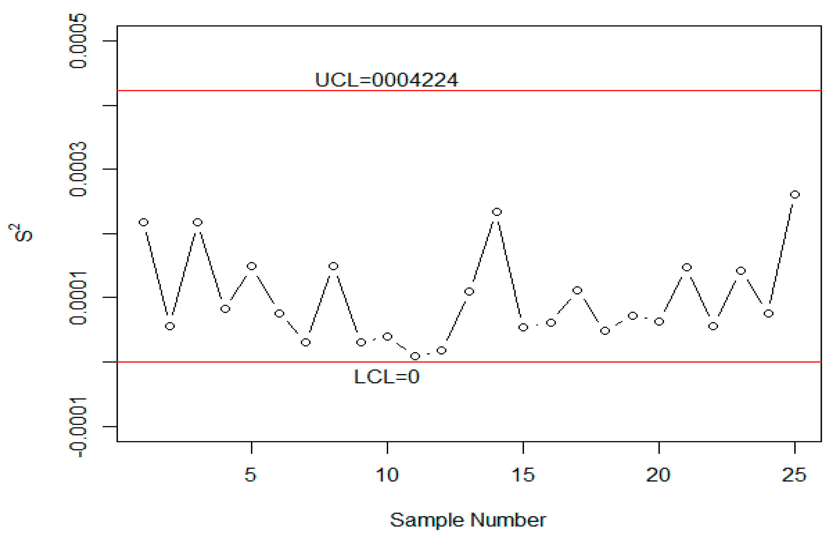
For this real example, suppose and = 370. The control limits of the proposed chart under the neutrosophic statistics are shown in Figure 3. We plotted the neutrosophic statistic in Figure 3. From Figure 3, it can be seen that although the process is in-control state, some plotting points are near the control limits. The control chart under the classical statistics is presented in Figure 4. From Figure 4, we note that the process is an in-control state with one point near the control limit. From Figure 3, we note that sample numbers 2, 7, 9, 10 and 11 are very close to . On the other hand, Figure 4 indicates that 11th and 12th sample numbers are very near to the LCL. By comparing Figure 3 with Figure 4, it can be concluded that although the plotting statistic is an in-control state, several points near the control limits need attention.
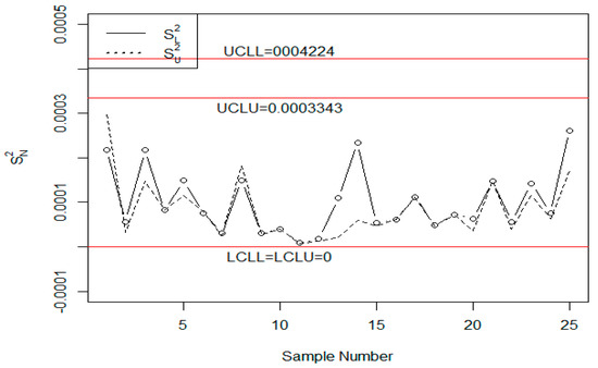
Figure 3.
The proposed plan using real data.
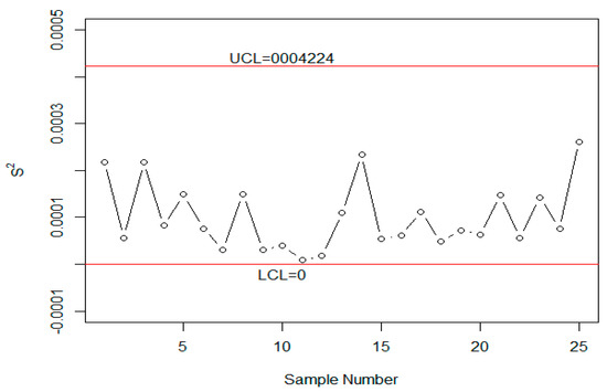
Figure 4.
The existing chart for the real data.
5. Concluding Remarks
We presented the designing of control chart under the neutrosophic interval statistical method. Some necessary measures to assess the performance of the proposed control chart are given. The advantages of the proposed control chart over the chart using the classical statistics are given. From the comparison, it is concluded that the proposed control chart is more effective and adequate under the uncertainty environment. The simulation study showed that the proposed chart has the ability to detect a shift in the process. The implementation of the proposed chart on the real data also shows its efficacies over the existing control chart. Therefore, it is recommended to apply the proposed control when the observations or the parameters are fuzzy. From the comparison and real example, it is concluded that the proposed chart under the neutrosophic statistics is quite adequate and effective in the uncertainty environment, more so than the method based on classical statistics. The proposed control chart using the exponentially weighted moving average (EWMA) will be considered as future research.
Author Contributions
Conceived and designed the experiments, M.A.; N.K. and M.Z.K.; Performed the experiments, M.A. and N.K.; Analyzed the data, M.A. and N.K.; Contributed reagents/materials/analysis tools, M.A.; Wrote the paper, M.A.
Funding
This article was funded by the Deanship of Scientific Research (DSR) at King Abdulaziz University, Jeddah. The authors, therefore, acknowledge with thanks DSR technical and financial support.
Acknowledgments
The authors are deeply thankful to the editor and reviewers for their valuable suggestions to improve the quality of this manuscript.
Conflicts of Interest
The authors declare no conflict of interest regarding this paper.
References
- Abbas, N.; Riaz, M.; Mahmood, T. An improved S2 control chart for cost and efficiency optimization. IEEE Access 2017, 5, 19486–19493. [Google Scholar] [CrossRef]
- RA, F. Statistical method from the viewpoint of quality control. Nature 1940, 146, 150. [Google Scholar]
- Khoo, M.B. S2 control chart based on double sampling. Int. J. Pure Appl. Math. 2004, 13, 249–258. [Google Scholar]
- Zhang, L.; Bebbington, M.; Lai, C.-D.; Govindaraju, K. On statistical design of the S2 control chart. Commun. Stat. Theory Methods 2005, 34, 229–244. [Google Scholar] [CrossRef]
- Khoo, M.B. A modified S chart for the process variance. Qual. Eng. 2005, 17, 567–577. [Google Scholar] [CrossRef]
- Lee, P.-H.; Chang, Y.-C.; Torng, C.-C. A design of S control charts with a combined double sampling and variable sampling interval scheme. Commun. Stat. Theory Methods 2012, 41, 153–165. [Google Scholar] [CrossRef]
- Riaz, M. A dispersion control chart. Commun. Stat. Simul. Comput. 2008, 37, 1239–1261. [Google Scholar] [CrossRef]
- Guo, B.; Wang, B.X. The design of the ARL-unbiased S2 chart when the in-control variance is estimated. Qual. Reliab. Eng. Int. 2015, 31, 501–511. [Google Scholar] [CrossRef]
- Zhang, G. Improved R and S control charts for monitoring the process variance. J. Appl. Stat. 2014, 41, 1260–1273. [Google Scholar] [CrossRef]
- Zadeh, L.A. Toward a generalized theory of uncertainty (GTU)––An outline. Inf. Sci. 2005, 172, 1–40. [Google Scholar] [CrossRef]
- Senturk, S.; Erginel, N. Development of fuzzy X¯~-R~ and X¯~-S~ control charts using α-cuts. Inf. Sci. 2009, 179, 1542–1551. [Google Scholar] [CrossRef]
- Rowlands, H.; Wang, L.R. An approach of fuzzy logic evaluation and control in SPC. Qual. Reliab. Eng. Int. 2000, 16, 91–98. [Google Scholar] [CrossRef]
- El-Shal, S.M.; Morris, A.S. A fuzzy rule-based algorithm to improve the performance of statistical process control in quality systems. J. Intell. Fuzzy Syst. 2000, 9, 207–223. [Google Scholar]
- Zabihinpour, M.; Tang, S.H.; Mohd ariffin, M.K.A.; Azfanizam, A.S. Construction of fuzzy −X-S control charts with an unbiased estimation of standard deviation for a triangular fuzzy random variable. J. Intell. Fuzzy Syst. 2015, 28, 2735–2747. [Google Scholar] [CrossRef]
- Shu, M.-H.; Dang, D.-C.; Nguyen, T.-L.; Hsu, B.-M.; Phan, N.C. Fuzzy and control charts: A data-adaptability and human-acceptance approach. Complexity 2017, 2017, 4376809. [Google Scholar] [CrossRef]
- Afshari, R.; Sadeghpour Gildeh, B. Designing a multiple deferred state attribute sampling plan in a fuzzy environment. Am. J. Math. Manag. Sci. 2017, 36, 328–345. [Google Scholar] [CrossRef]
- Fadaei, S.; Pooya, A. Fuzzy U control chart based on fuzzy rules and evaluating its performance using fuzzy OC curve. TQM J. 2018, 30, 232–247. [Google Scholar] [CrossRef]
- Ercan Teksen, H.; Anagun, A.S. Different methods to fuzzy X¯-R control charts used in production: Interval type-2 fuzzy set example. J. Enterp. Inf. Manag. 2018, 31, 848–866. [Google Scholar] [CrossRef]
- Smarandache, F. Neutrosophic logic—A generalization of the intuitionistic fuzzy logic. arXiv, 2003; arXiv:math/0303009. [Google Scholar]
- Smarandache, F. Introduction to neutrosophic statistics. arXiv, 2014; arXiv:1406.2000. [Google Scholar]
- Chen, J.; Ye, J.; Du, S. Scale effect and anisotropy analyzed for neutrosophic numbers of rock joint roughness coefficient based on neutrosophic statistics. Symmetry 2017, 9, 208. [Google Scholar] [CrossRef]
- Chen, J.; Ye, J.; Du, S.; Yong, R. Expressions of rock joint roughness coefficient using neutrosophic interval statistical numbers. Symmetry 2017, 9, 123. [Google Scholar] [CrossRef]
- Aslam, M. A new sampling plan using neutrosophic process loss consideration. Symmetry 2018, 10, 132. [Google Scholar] [CrossRef]
- Aslam, M.; Arif, O. Testing of grouped product for the weibull distribution using neutrosophic statistics. Symmetry 2018, 10, 403. [Google Scholar] [CrossRef]
- Montgomery, D.C. Introduction to Statistical Quality Control; John Wiley & Sons: New York, NY, USA, 2007. [Google Scholar]
© 2018 by the authors. Licensee MDPI, Basel, Switzerland. This article is an open access article distributed under the terms and conditions of the Creative Commons Attribution (CC BY) license (http://creativecommons.org/licenses/by/4.0/).