Abstract
The hybrid synchronization problem of a class of chaotic systems is investigated in this paper. Firstly, the existence of hybrid synchronization problems in such systems is proved theoretically by a proposed necessary and sufficient condition. That is, the hybrid synchronization problem is equivalent to solve a group of nonlinear algebraic equations about . It is interesting that one value of indicates one type of synchronization. Secondly, all solutions for the hybrid synchronization problem are obtained by finding solutions of all the above equations about . Thirdly, an universal control method is proposed to realize such hybrid synchronization problems. Finally, illustrative examples are provided to verify the validity and effectiveness of the obtained results.
1. Introduction
It is believed that the strange attractor and butterfly effect proposed by Lorenz in 1963 could help people begin to keep an eye on chaotic dynamics and even be used in nonlinear science. From then on, chaotic behavior has been extensively analyzed in many fields, e.g., engineering, ecology, biology, economics, and so on, even in the social sciences. More attention has been paid to these problems associated with synchronization and control of chaotic systems since the significant works carried out by Pecora and Carroll in 1990 [1,2]. It is well known that complete synchronization of unidirectionally coupled chaotic systems and its potential applications in engineering are currently a field of great interest. Also, projective synchronization has received much attention due to its faster communication and proportionality between the dynamical systems. In case of projective synchronization, the master and the slave system can be synchronized up to a scaling factor. The scaling factor is a constant transformation between the driving and the response variables. In applying this to secure communications, this proportional feature can be used to extend binary digital to M-nary digital communication for getting communication much faster. In conclusion, the relevant topics about chaotic and even hyper-chaotic systems could cover these subjects such as (1) emergence and occurrence of chaotic attractors, multi-scroll attractors, multi-wings, in continuous dynamic systems or maps; (2) chaos in integer and/or fractional order nonlinear systems; (3) spatiotemporal chaos in coupled oscillators or network; (4) Chaotic properties in electric activities of neurons; (5) Chaos control and synchronization problems. The emergence of chaos and hyper-chaos in dynamic systems could be harmful for us and should be controlled. In this case, many schemes were proposed to apply the chaotic systems to reach arbitrary orbits or stable points. Indeed, the self-adaptive control scheme is appreciated greatly because the controller could have lower power consumption and take a shorter transient period to reach the goal. In the last decades, this topic has been extensively investigated, some interesting research can be explored in relevant works [1,2,3,4,5,6,7,8,9,10,11,12,13,14,15,16,17,18,19,20,21,22,23,24,25,26] and many similar results have been cited in those references. However, there still exist many important problems which have not been considered in the existing literatures.
In the next, we take the following example to show it. Consider the following hyper-chaotic system [4]:
where , are real numbers.
Following the procedures in [4], the slave system is given as follows:
where is the designed controller which can meet the desires performance.
Define the following sum variables:
then the sum system is obtained as follows:
According to the results in [4], the designed controllers are presented as follows:
where are given as follows:
It is well known that the controller is designed in this form: , where and , which is a physically implementable. In general, the single input controller is usually designed in real applications, i.e., . It is easy to see that the designed controller (4) is not a physically implementable controller because that the dimension of this controller is the same as the dimension of the system (3). Moreover, it is obvious that the sub-controllers (5) are only used to counteract the corresponding opposite terms in the sum system (3). Similar results published in [5,6,7,8,9,10,11], the designed controllers can guarantee the performance: the anti-synchronization, but the designed controllers are only mathematically relevant in some sense. In a word, the anti-synchronization problem for a given chaotic system should be investigated firstly when this system is considered. In fact, we have proved rigorously the fact: for a given chaotic system in this form: , where , the anti-synchronization problem exists if and only if in [26]. Therefore, there are still exist many important problems for the chaotic systems in arbitrary dimensions which need to be investigated further.
Up to now, there are several types of synchronization problems for the chaotic systems, e.g., anti-synchronization, synchronization, projective synchronization, coexistence of synchronization and anti-synchronization, simultaneous synchronization and anti-synchronization, etc. In [25], we have investigated the projective synchronization problem for a class of chaotic systems extensively. A natural question arises: can several types of synchronization problems for a given chaotic system be investigated in a unified form? i.e., whether the complete synchronization, anti-synchronization, coexistence of synchronization and anti-synchronization, simultaneous anti-synchronization and complete synchronization, are studied in a unified form or not? This question is very important in theory and applications. To the best of the authors’ knowledge, there are no relative literatures have been published so far, which motivates us to do the present work.
As is stated in [9], the existence of hybrid synchronization can effectively enhance security in communication. Due to these reasons, to design the proper controller to reach the hybrid synchronization has become an important problem. Therefore, we investigate the hybrid synchronization problem of a class of chaotic systems and present serval new results. The main contributions are summarized as follows: (1) A new unified definition named hybrid synchronization is presented; (2) A necessary and sufficient condition is proposed, which is used to proof the existence of the hybrid synchronization problem of the chaotic systems. Based on this condition, the hybrid synchronization problem is equivalent to solve a group of nonlinear algebraic equations about , i.e., one value of indicates one type of synchronization problem; (3) All solutions for the hybrid synchronization problem are obtained by finding solutions of all algebraic equations about ; (4) An universal control method is designed to ensure the realization the hybrid synchronization problem (see Figure 1).
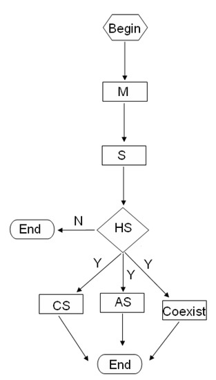
Figure 1.
The flowchart of proposed technique.
Remark 1.
M and S stand for the master system and the slave system, respectively. Hybrid Synchronization (HS), Complete Synchronization (CS), Anti-Synchronization (AS), Coexistence of complete synchronization and anti-synchronization (Coexist).
Notation Throughout this paper, as usual, stands for the real number, represents an identity matrix, is an index set, is a diagonal matrix, where , and is a controller, where is a continuous vector function with = 0.
2. Preliminaries and Problem Formation
We firstly present a new unified definition for the sequel use.
Consider the chaotic system which is expressed as follows:
where , is a continuous function vector and .
Suppose the system (6) be the master system, then the slave system with variable y is given as:
where , is the designed controller.
Make , and then the error system is presented as follows:
where is the state vector.
Summarizing the existing definitions in [26,27,28], we give a new unified definition named hybrid synchronization in the next.
Definition 1.
Consider the error system (8).
- If holds for the case: some = 1, while the rest = −1, , then the system (6) and the system (7) are called to achieve the coexistence of synchronization and anti-synchronization, i.e., some variables: , anti-synchronize the corresponding variables: , while the rest variables: , synchronize the corresponding variables: , .
- If holds simultaneously for the two cases: and , then the system (6) and the system (7) are called to achieve simultaneous synchronization and anti-synchronization, i.e., if the system (6) and the system (7) are anti-synchronized by the controller in this form: , then these two systems are also synchronized by the controller in this form: , vice versa.
3. Main Results
3.1. The Existence of the Hybrid Synchronization Problem for a Class of Chaotic Systems
To design the physically implementable controller, should be an equilibrium point of the following error system which is uncontrolled (i.e., ):
it results in
i.e.,
In the next, a conclusion is presented as follows.
Theorem 1.
The existence of the hybrid synchronization problem for the system (6) if and only if: have solutions about α.
Proof:
⟸
Since the equations: have solutions about , then is an equilibrium point of the system (9) is induced. According to the nonlinear control theory, a physically implementable controller can be designed to stabilize the system (9), and thus the hybrid synchronization problem of the system (6) is realized.
⟹
Remark 3.
It should be pointed out that there exists at least one solution satisfying Equation (11) about α: , i.e., .
Classifying all the solutions of Equation (11) about : , we present the results as follows.
Corollary 1.
Corollary 2.
With Corollary 2 and Definition 1, we present the following result.
Corollary 3.
The anti-synchronization problem of the system (6) exists .
With the results in [28], Corollary 3 and Definition 1, the following result is obtained.
Corollary 4.
If , then the simultaneous anti-synchronization and complete synchronization problem of the system (6) exists.
Then, according to the results in [25], the following corollary is presented.
Corollary 5.
Remark 4.
In this case, , which implies that is a linear function. As we know that all chaotic systems are nonlinear. Therefore, it is impossible for the whole chaotic system to realize the projective synchronization by a physically implementable controller. As a matter of fact, only some subsystem which has some partial linear variables can achieve projective synchronization, which is the same to the existing results in [29]. Thus, the projective synchronization is not investigated here, for details, please see our latest paper [25].
According to the results in [30], the following conclusion is obtained.
Corollary 6.
For some chaotic systems which satisfy special conditions, we can prove the existence of the coexistence of synchronization and anti-synchronization problem for those systems directly. Then, the following results are proposed.
Theorem 2.
Consider the system (6). If , and there exists a non-singular transformation: by which the system (6) is rewritten as follows:
where , , and is an even function, , then the master system
and the slave system
can achieve the coexistence of synchronization and anti-synchronization in the following two cases:
Proof:
Let and , then the uncontrolled (i.e., ) error system is presented as follows:
If , i.e., , then we obtain
By a same argument, we obtain
i.e., the origin is an equilibrium point of the system (15). Therefore, a physically implementable controller u can be designed to stabilize the system (15).
For the other case, we can prove it by a similar procedure, which completes the proof. □
Theorem 3.
Consider the system (6). If there exists a non-singular transformation: by which the system (6) is transferred into the following system:
where , , and is an even function about M, i.e., , then the master system
and the slave system
can achieve the following coexistence of synchronization and anti-synchronization:
Proof:
Let and , then the uncontrolled (i.e., ) error system is given as
If , i.e., , , then we obtain
3.2. Solutions of the Hybrid Synchronization Problem for a Given Chaotic System
In this subsection, for a given chaotic system, the solutions of the hybrid synchronization problem of such system are investigated. Solving Equation (11) about : , i.e., finding the solutions of a group of nonlinear algebraic equations about , we can obtain all solutions: , where . It is interesting that one value of indicates one type of synchronization, e.g., , which implies that the complete synchronization problem can be realized, and , which indicates that the anti-synchronization problem can be achieved, and so on. In Section 4, we shall take two examples to show it in detail.
3.3. The Implementation of the Hybrid Synchronization for the Given Chaotic Systems
It is well known that there are many methods to realize the hybrid synchronization problem for the given chaotic systems, but the adaptive control method is applied easily in applications. In the following, we extend the our previous method [3] to solve this problem, and give the follow result.
Theorem 4.
For the error system (9), if there exists a non-singular transformation: which can divide the system (9) into the following two subsystems:
where , , , and the following subsystem:
is globally asymptotically stable, then the designed controller is given as
and the dynamic gain is evolved by the following update law:
where which is chosen in advance. That is to say, the following system:
is globally asymptotically stable, which indicates that the hybrid synchronization problem of the system (6) is achieved.
4. Examples with Numerical Simulations
In this section, two examples are provided to demonstrate how to investigate several types of synchronization problem by the obtained results in this paper.
Example 1.
The 4D hyper-chaotic system [31]:
Solving Equation (28) about , we obtain the following four solutions:
Case 1: , which indicates that complete synchronization problem of the system (25) exists;
Case 2: , which implies that anti-synchronization problem of the system (25) exists;
Case 3: while , which indicates that the coexistence of synchronization and anti-synchronization problem of the system (25) exists;
Case 4: while , which implies that the coexistence of synchronization and anti-synchronization problem of the system (25) exists.
Remark 5.
Summarizing Case 1 and Case 2, the simultaneous anti-synchronization and synchronization for the system (25) can be achieved, which is the same to our existing results in [28]. It is noted that there exist two cases of the coexistence of synchronization and anti-synchronization for the system (25) by summarizing Case 3 and Case 4.
On the other hand, if let , ,
and noticing that , then we can also present the same results as the above ones: Case 3 and Case 4, according to Theorem 2.
In the next, by applying the adaptive control method [3], we shall investigate how to design an universal controller to achieve the hybrid synchronization.
According to the results in Section 2, let the system (25) be master system, then the corresponding uncontrolled slave system with variable y is described as follows:
Then, let , where meets the Equation (28), , thus the uncontrolled error system is presented in the following:
Obviously, if , then the remainder subsystem of system (30):
is globally asymptotically stable whatever is.
With Theorem 4, the controlled error system is presented as
i.e., the controller is designed as follows:
and the dynamic feedback is evolved by the following update law:
where .
In the next, choose following initial conditions: = , = , and . The simulation results are shown by the following figures.
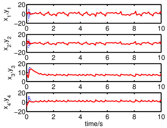
It can be seen from Figure 2 and Figure 3 that the complete synchronization between the master system (25) and the slave system (29) has been realized by the controller (32).
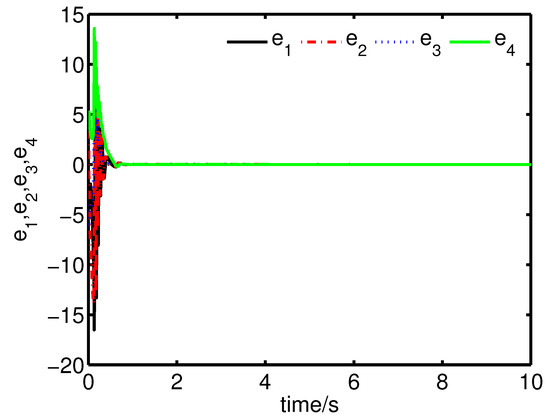
Figure 2.
The states of the error system (31) converge to origin as .
It can be seen from Figure 4 and Figure 5 that the anti-synchronization between the master system (25) and the slave system (29) has been realized by the controller (32).
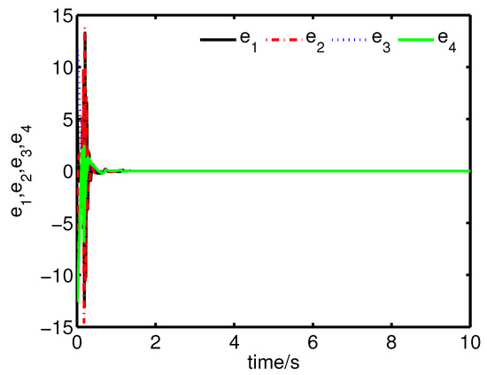
Figure 4.
The states of the error system (31) converge to origin as .
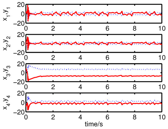
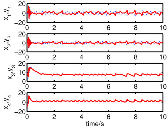
It can be seen from Figure 6 and Figure 7 that the complete synchronization between the master system (25) and the slave system (29) has been realized by the controller (32).
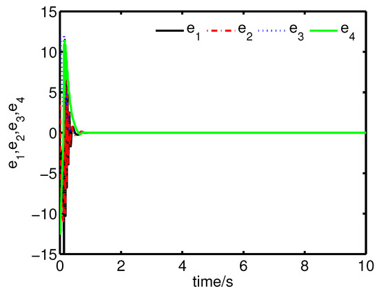
Figure 6.
The states of the error system (31) converge to origin as .
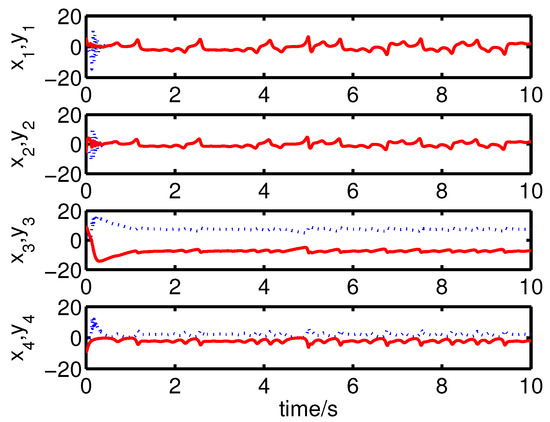
It can be seen from Figure 8 and Figure 9 that the complete synchronization between the master system (25) and the slave system (29) has been realized by the controller (32).
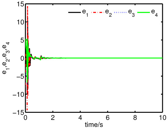
Figure 8.
The states of the error system (31) converge to origin as .
Example 2.
The Lorenz system [32]:
Solving Equation (36) about , two solutions are presented as follows:
Case 1: , which indicates that the complete synchronization problem of the system (34) exists;
Case 2: , while , which implies that the coexistence of synchronization and anti-synchronization problem of the the system (34) exists.
Remark 6.
In conclusion, there is no any other solution satisfying the Equation (36). Thus, Example 2 shows that it is impossible for the whole chaotic system to realize anti-synchronization if is not an odd function by a physically implementable controller.
In the next, the the hybrid synchronization of the Lorenz system (34) is investigated as follows.
Similarly, make the system (34) be the master system, then the uncontrolled slave system with variable y is described as follows:
Then, let , where , , satisfies Equation (36), then the uncontrolled error system is presented in the following:
Obviously, if , then the remainder subsystem of system (38):
is globally asymptotically stable whatever is.
With Theorem 4, the controlled error system is given as:
i.e., the controller is designed as follows:
and the dynamic feedback is evolved by the following update law:
where .
In the next, select following initial conditions: = , = , and , . The simulation results are showed as the following figures.
It can be seen from Figure 10 and Figure 11 that the complete synchronization between the master system (34) and the slave system (37) has been realized by the controller (40).
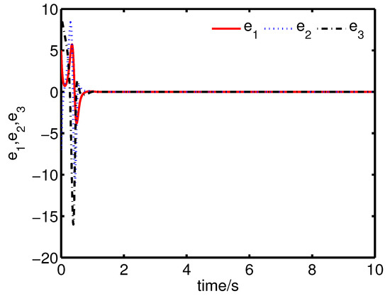
Figure 10.
The states of the error system (39) converge to origin as .
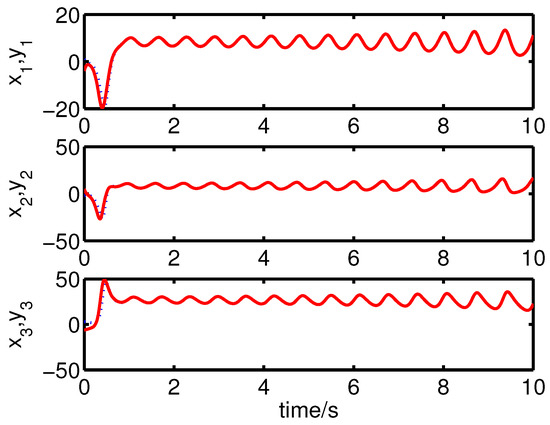
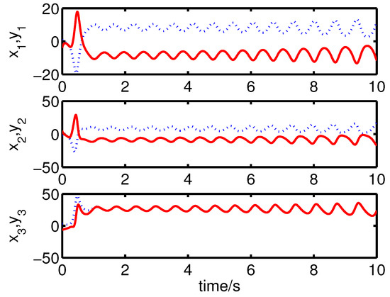
It can be seen from Figure 12 and Figure 13 that the coexistence of synchronization and anti-synchronization between the master system (34) and the slave system (37) has been realized by the controller (40).
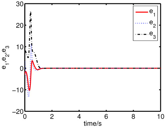
Figure 12.
The states of the error system (39) converge to origin as .
5. Conclusions
The hybrid synchronization problem for a class of chaotic systems has been investigated extensively. Firstly, we have proposed a necessary and sufficient condition to guarantee the existence of the hybrid synchronization problem. Based on this, such problems are equivalent to solve a group of nonlinear algebraic equations about . It should be pointed out that one value of indicates one type of synchronization, which is very interesting. Secondly, we have found all solutions for the hybrid synchronization problem by finding solutions of all nonlinear algebraic equations about . Moreover, we have designed an universal control method to realize the hybrid synchronization problem. Finally, numerical examples have been provided to verify the validity and effectiveness of the proposed theoretical results.
We hope the obtained theoretical results in this paper can be applied to the hybrid synchronization of the complex networks and some other relative nonlinear systems.
Author Contributions
Z.W. deals with the numerical simulation, R.G. deduces the main results and writes this paper.
Funding
This work is supported by Shandong Natural Science Foundation [ZR2018MF016] and National Natural Science Foundation of China [61877062].
Acknowledgments
The authors would like to thank the anonymous Reviewers and the Editors for their constructive comments and suggestions, which have helped enhance the presentation of this paper.
Conflicts of Interest
The authors declare no conflict of interest.
References
- Ott, E.; Gerbogi, C.; Yorke, J.A. Controlling Chaos. Phys. Rev. Lett. 1990, 64, 1196–1199. [Google Scholar] [CrossRef] [PubMed]
- Pecora, L.; Carroll, T. Synchronization in Chaotic Systems. Phys. Rev. Lett. 1990, 64, 821–824. [Google Scholar] [CrossRef] [PubMed]
- Guo, R. A simple adaptive controller for chaos and hyperchaos synchronization. Phys. Lett. A 2008, 372, 5593–5597. [Google Scholar] [CrossRef]
- Al-Sawalha, M.M.; Noorani, M.S.M. Anti-synchronization of two hyperchaotic systems via nonlinear control. Commun. Nonlinear Sci. Numer. Simul. 2009, 14, 3402–3411. [Google Scholar] [CrossRef]
- Wang, Z.F.; Shi, X.R. Anti-synchronization of Liu system and Lorenz system with known and unknown parameters. Nonlinear Dyn. 2009, 57, 425–430. [Google Scholar] [CrossRef]
- Al-Sawalha, M.M.; Noorani, M.S.M. Adaptive anti-synchronization of two identical and different hyperchaotic systems with uncertain parameters. Commun. Nonlinear Sci. Numer. Simul. 2010, 15, 1036–1047. [Google Scholar] [CrossRef]
- Al-Sawalha, M.M.; Noorani, M.S.M. Adaptive reduced-order anti-synchronization of chaotic systems with fully unknown parameters. Commun. Nonlinear Sci. Numer. Simul. 2010, 15, 3022–3034. [Google Scholar] [CrossRef]
- Bhatnagar, G.; Wu, Q.M.J. A novel chaos based secure transmission of biometric data. Neurocomputing 2015, 147, 444–455. [Google Scholar] [CrossRef]
- Chen, X.Y.; Qiu, J.L.; Cao, J.D.; He, H.B. Hybrid synchronization behavior in an array of coupled chaotic systems with ring connection. Neurocomputing 2016, 173, 1299–1309. [Google Scholar] [CrossRef]
- Ma, J.; Wu, F.Q.; Ren, G.D.; Tang, J. A class of initials-dependent dynamical systems. Appl. Math. Comput. 2017, 298, 65–76. [Google Scholar] [CrossRef]
- Wu, F.Q.; Hayat, T.; An, X.L.; Ma, J. Can Hamilton energy feedback suppress the chameleon chaotic flow? Nonlinear Dyn. 2018, 94, 669–677. [Google Scholar] [CrossRef]
- Huang, L.Y.; Hwang, S.S.; Bae, Y.C. Chaotic Behavior in Model with a Gaussian Function as External Force. Int. J. Fuzzy Log. Intell. Syst. 2016, 16, 262–269. [Google Scholar] [CrossRef]
- Qi, G.Y.; Hu, J.B. Force Analysis and Energy Operation of Chaotic System of Permanent-Magnet Synchronous Motor. Int. J. Bifurc. Chaos 2017, 27, 1750216. [Google Scholar] [CrossRef]
- Yuan, Z.S.; Li, H.T.; Miao, Y.C. Digital-Analog Hybrid Scheme and Its Application to Chaotic Random Number Generators. Int. J. Bifurc. Chaos 2017, 27, 1750210. [Google Scholar] [CrossRef]
- Xu, C.B.; Yang, R.H. Parameter estimation for chaotic systems using improved bird swarm algorithm. Mod. Phys. Lett. B 2017, 31, 1750346. [Google Scholar] [CrossRef]
- Gotoda, H.; Pradas, M.; Kalliadasis, S. Chaotic versus stochastic behavior in active-dissipative nonlinear systems. Phys. Rev. Fluids 2017, 31, 124401. [Google Scholar] [CrossRef]
- Gao, W.; Yan, L.; Saeedi, M. Ultimate bound estimation set and chaos synchronization for a financial risk system. Math. Comput. Simul. 2018, 154, 19–33. [Google Scholar] [CrossRef]
- Wang, M.X.; Wang, X.Y.; Zhang, Y.Q. A novel chaotic encryption scheme based on image segmentation and multiple diffusion models. Opt. Laser Technol. 2018, 108, 558–573. [Google Scholar] [CrossRef]
- Wang, J.; Shi, K.B.; Huang, Q.Z. Stochastic switched sampled-data control for synchronization of delayed chaotic neural networks with packet dropout. Appl. Math. Comput. 2018, 335, 211–230. [Google Scholar] [CrossRef]
- Gayathri, J.; Subashini, S. A spatiotemporal chaotic image encryption scheme based on self adaptive model and dynamic keystream fetching technique. Multimedia Tools Appl. 2018, 77, 24751–24787. [Google Scholar] [CrossRef]
- Hua, Z.Y.; Zhou, B.H.; Zhou, Y.C. Sine chaotification model for enhancing chaos and its hardware implementation. IEEE Trans. Ind. Electron. 2019, 66, 1273–1284. [Google Scholar] [CrossRef]
- Kuznetsov, S.P.; Kruglov, V.P. Hyperbolic chaos in a system of two Froude pendulums with alternating periodic braking. Commun. Nonlinear Sci. Numer. Simul. 2019, 67, 152–161. [Google Scholar] [CrossRef]
- Gardini, L.; Makrooni, R. Necessary and sufficient conditions of full chaos for expanding Baker-like maps and their use in non-expanding Lorenz maps. Commun. Nonlinear Sci. Numer. Simul. 2019, 67, 272–289. [Google Scholar] [CrossRef]
- Zhou, J.; Zhou, W.; Chu, T. Bifurcation, intermittent chaos and multi-stability in a two-stage Cournot game with R&D spillover and product differentiation. Appl. Math. Comput. 2019, 341, 358–378. [Google Scholar]
- Guo, R.W. Projective synchronization of a class of chaotic systems by dynamic feedback control method. Nonlinear Dyn. 2017, 90, 53–64. [Google Scholar] [CrossRef]
- Ren, L.; Guo, R.W. A necessary and sufficient condition of anti-synchronization for chaotic systems and its applications. Math. Probl. Eng. 2015, 2015. [Google Scholar] [CrossRef]
- Ren, L.; Guo, R.W.; Vincent, U.E. Coexistence of synchronization and anti-synchronization in chaotic systems. Arch. Control Sci. 2016, 26, 69–79. [Google Scholar] [CrossRef]
- Guo, R.W. Simultaneous synchrnizaiton and anti-synchronzation of two identical new 4D chaotic systems. Chin. Phys. Lett. 2011, 28. [Google Scholar] [CrossRef]
- Mainieri, R.; Rehacke, J. Projective synchronization in three-dimensional chaotic oscillators. Phys. Rev. Lett. 1999, 82, 3042–3045. [Google Scholar] [CrossRef]
- Zhang, Q.; Lü, J.; Chen, S. Coexistence of anti-phase and complete synchronization in the generalized Lorenz system. Commun. Nonlinear Sci. Numer. Simul. 2010, 15, 3067–3072. [Google Scholar] [CrossRef]
- Qi, G.Y.; Du, S.Z.; Chen, G.R.; Chen, Z.Q.; Yuan, Z.Z. On a four-dimensional chaotic system. Chaos Solitons Fractals 2005, 23, 1671–1682. [Google Scholar] [CrossRef]
- Lorenz, E.N. Deterministic nonperiodic flow. J. Atmos. Sci. 1963, 20, 130–141. [Google Scholar] [CrossRef]


© 2018 by the authors. Licensee MDPI, Basel, Switzerland. This article is an open access article distributed under the terms and conditions of the Creative Commons Attribution (CC BY) license (http://creativecommons.org/licenses/by/4.0/).