Visual Simulation of Detailed Turbulent Water by Preserving the Thin Sheets of Fluid


Abstract
:1. Introduction
2. Related Work
3. Preserving the Thin Sheet and Turbulence Details of Water
- 1.
- Water particles are advected and their density is calculated.
- 2.
- Singular value decomposition (SVD) is used to extract thin particles from water particles.
- 3.
- The distances and relative velocities between thin particle pairs are used to find candidate positions.
- 4.
- The candidate positions are used to insert and break new water particles.
- 5.
- To restore the missing turbulence, the ghost density is calculated for all of the water particles, including the newly inserted water particles. The ghost mass is then calculated based on the density to ensure the conservation of mass.
- 6.
- The ghost mass is used to rasterize the velocities of particles on an Eulerian grid and advect the water particles using a FLIP solver.
- 7.
- The fluid surfaces are reconstructed.
3.1. Preserving Thin Sheets
3.1.1. Extracting Thin Particles
3.1.2. Finding Candidate Positions
3.1.3. Inserting and Removing Particles
3.2. Synthesizing Turbulence Details
4. Implementation
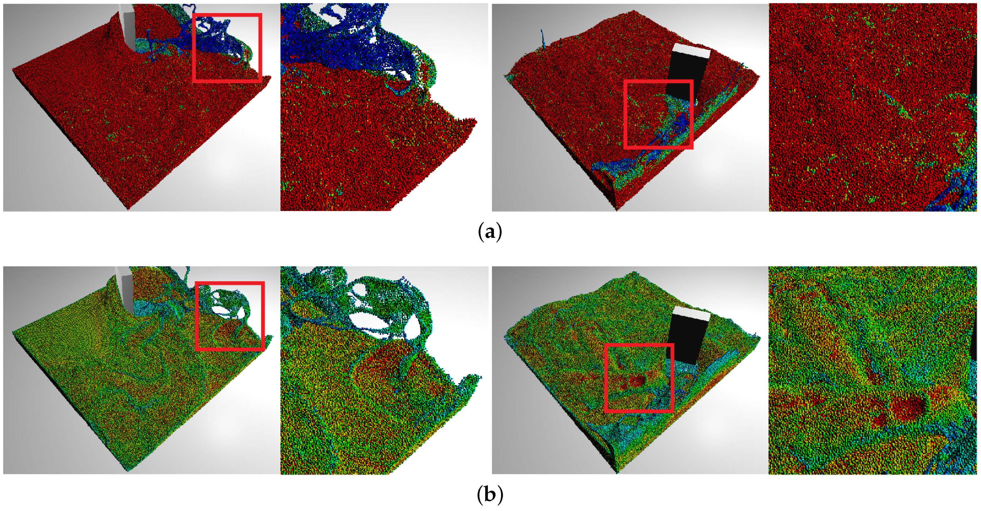
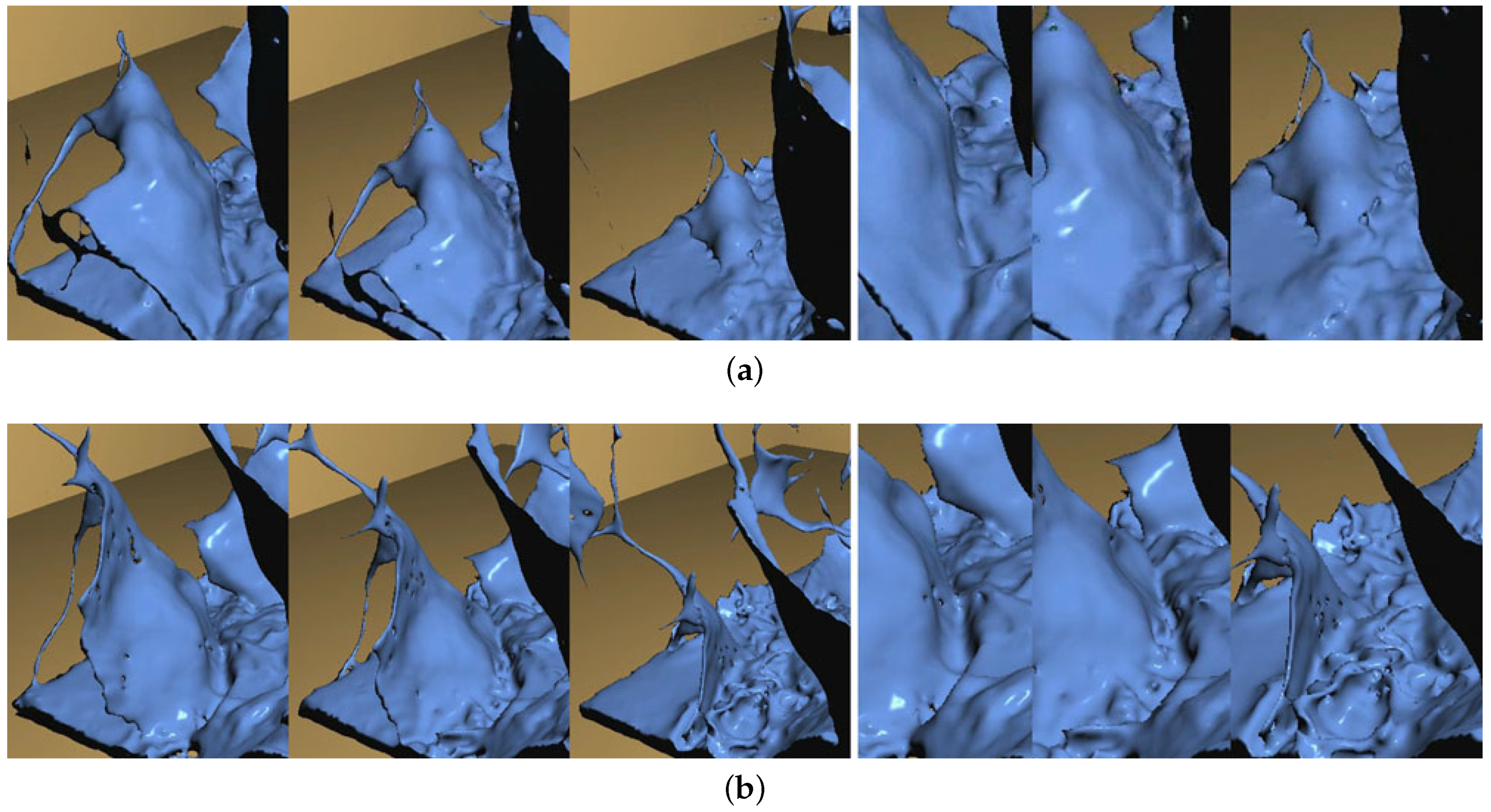
5. Results
6. Discussion and Additional Explanation
7. Conclusions
Author Contributions
Funding
Conflicts of Interest
References
- Chen, F.; Zhao, Y.; Yuan, Z. Langevin particle: A selfadaptive lagrangian primitive for flow simulation enhancement. Comput. Gr. Forum 2011, 30, 435–444. [Google Scholar] [CrossRef]
- Zhao, Y.; Yuan, Z.; Chen, F. Enhancing fluid animation with adaptive, controllable and intermittent turbulence. In Proceedings of the ACM SIGGRAPH/Eurographics Symposium on Computer Animation, Madrid, Spain, 2–4 July 2010; pp. 75–84. [Google Scholar]
- Selle, A.; Rasmussen, N.; Fedkiw, R. A Vortex Particle Method for Smoke, Water and Explosions; ACM SIGGRAPH: New York, NY, USA, 2005; pp. 910–914. [Google Scholar]
- Yoon, J.-C.; Kam, H.R.; Hong, J.-M.; Kang, S.J.; Kim, C.-H. Procedural synthesis using vortex particle method for fluid simulation. Compt. Gr. Forum 2009, 28, 1853–1859. [Google Scholar] [CrossRef]
- Kim, D.; Lee, S.W.; Young Song, O.; Ko, H.S. Baroclinic turbulence with varying density and temperature. IEEE Trans. Vis. Comput. Gr. 2012, 18, 1488–1495. [Google Scholar]
- Weissmann, S.; Pinkall, U. Filament-based smoke with vortex shedding and variational reconnection. ACM Trans. Gr. 2010, 29, 115–122. [Google Scholar] [CrossRef]
- Barnat, A.; Pollard, N.S. Smoke sheets for graph-structured vortex filaments. In Proceedings of the ACM SIGGRAPH/Eurographics Symposium on Computer Animation, Lausanne, Switzerland, 29–31 July 2012; pp. 77–86. [Google Scholar]
- Hong, J.M.; Shinar, T.; Fedkiw, R. Wrinkled Flames and Cellular Patterns; ACM SIGGRAPH: New York, NY, USA, 2007; Volume 26, pp. 47–54. [Google Scholar]
- Kim, D.; Song, O.Y.; Ko, H.S. Stretching and Wiggling Liquids; ACM SIGGRAPH Asia: New York, NY, USA, 2009; pp. 120:1–120:7. [Google Scholar]
- Mercier, O.; Beauchemin, C.; Thuerey, N.; Kim, T.; Nowrouzezahrai, D. Surface Turbulence for Particle-Based Liquid Simulations. ACM Trans. Gr. 2015, 34, 10–16. [Google Scholar] [CrossRef]
- Pfaff, T.; Thuerey, N.; Gross, M. Lagrangian vortex sheets for animating uids. ACM Trans. Gr. 2012, 31, 112:1–112:8. [Google Scholar] [CrossRef]
- Pfaff, T.; Thuerey, N.; Cohen, J.; Tariq, S.; Gross, M. Scalable Fluid Simulation Using Anisotropic Turbulence Particles; ACM SIGGRAPH Asia: New York, NY, USA, 2010; pp. 174:1–174:8. [Google Scholar]
- Kim, T.; Thürey, N.; James, D.; Gross, M. Wavelet Turbulence for Fluid Simulation; ACM SIGGRAPH: New York, NY, USA, 2008; pp. 50:1–50:6. [Google Scholar]
- Pfaff, T.; Thuerey, N.; Selle, A.; Gross, M. Synthetic Turbulence Using Artificial Boundary Layers; ACM SIGGRAPH Asia: New York, NY, USA, 2009; pp. 121:1–121:10. [Google Scholar]
- Dobashi, Y.; Matsuda, Y.; Yamamoto, T.; Nishita, T. A fast simulation method using overlapping grids for interactions between smoke and rigid objects. Comput. Gr. Forum 2008, 27, 477–486. [Google Scholar] [CrossRef]
- Klingner, B.M.; Feldman, B.E.; Chentanez, N.; O’Brien, J.F. Fluid Animation With Dynamic Meshes; ACM SIGGRAPH: New York, NY, USA, 2006; pp. 820–825. [Google Scholar]
- Losasso, F.; Gibou, F.; Fedkiw, R. Simulating Water and Smoke With an Octree Data Structure; ACM SIGGRAPH: New York, NY, USA, 2004; pp. 457–462. [Google Scholar]
- Jang, T.; Blanco i Ribera, R.; Bae, J.; Noh, J. Simulating sph fluid with multi-level vorticity. Int. J. Virtual Real. 2011, 10, 21–27. [Google Scholar]
- Yang, B.; Jin, X. Turbulence synthesis for shape-controllable smoke animation. Comput. Anim. Virtual Worlds 2014, 25, 465–472. [Google Scholar] [CrossRef]
- Zhu, B.; Yang, X.; Fan, Y. Creating and preserving vortical details in sph fluid. Comput. Gr. Forum 2010, 29, 2207–2214. [Google Scholar] [CrossRef]
- Ando, R.; Thurey, N.; Tsuruno, R. Preserving fluid sheets with adaptively sampled anisotropic particles. IEEE Trans. Vis. Comput. Gr. 2012, 18, 1202–1214. [Google Scholar] [CrossRef] [PubMed]
- Ando, R.; Tsuruno, R. A particle-based method for preserving fluid sheets. In Proceedings of the ACM SIGGRAPH/Eurographics Symposium on Computer Animation, Vancouver, British, 5–7 August 2011; pp. 7–16. [Google Scholar]
- Wojtan, C.; Thürey, N.; Gross, M.; Turk, G. Physics-Inspired Topology Changes for Thin Fluid Features; ACM SIGGRAPH: New York, NY, USA, 2010; pp. 50:1–50:8. [Google Scholar]
- Stam, J. Stable Fluids; ACM SIGGRAPH: New York, NY, USA, 1999; pp. 121–128. [Google Scholar]
- Fedkiw, R.; Stam, J.; Jensen, H.W. Visual Simulation of Smoke; ACM SIGGRAPH: New York, NY, USA, 2001; pp. 15–22. [Google Scholar]
- He, S.; Wong, H.C.; Pang, W.M.; Wong, U.H. Real-time smoke simulation with improved turbulence by spatial adaptive vorticity connement. Comput. Anim. Virtual Worlds 2011, 22, 107–114. [Google Scholar] [CrossRef]
- Park, S.I.; Kim, M.J. Vortex fluid for gaseous phenomena. In Proceedings of the ACM SIGGRAPH/Eurographics Symposium on Computer Animation, Los Angeles, CA, USA, 29–31 July 2005; pp. 261–270. [Google Scholar]
- Angelidis, A.; Neyret, F. Simulation of smoke based on vortex lament primitives. In Proceedings of the ACM SIGGRAPH/Eurographics Symposium on Computer Animation, Los Angeles, CA, USA, 29–31 July 2005; pp. 87–96. [Google Scholar]
- Angelidis, A.; Neyret, F.; Singh, K.; Nowrouzezahrai, D. A controllable, fast and stable basis for vortex based smoke simulation. In Proceedings of the ACM SIGGRAPH/Eurographics Symposium on Computer Animation, Vienna, Austria, 2–4 September 2006; pp. 25–32. [Google Scholar]
- Schechter, H.; Bridson, R. Evolving sub-grid turbulence for smoke animation. In Proceedings of the ACM SIGGRAPH/Eurographics Symposium on Computer Animation, Dublin, Ireland, 7–9 July 2008; pp. 1–7. [Google Scholar]
- Vines, M.; Houston, B.; Lang, J.; Lee, W.S. Vortical inviscid flows with two-way solid-fluid coupling. IEEE Trans. Vis. Comput. Gr. 2014, 20, 303–315. [Google Scholar] [CrossRef] [PubMed]
- Osher, S.; Sethian, J.A. Fronts propagating with curvature-dependent speed: Algorithms based on hamilton-jacobi formulations. J. Comput. Phys. 1988, 79, 12–49. [Google Scholar] [CrossRef]
- Enright, D.; Fedkiw, R.; Ferziger, J.; Mitchell, I. A hybrid particle level set method for improved interface capturing. J. Comput. Phys. 2002, 183, 83–116. [Google Scholar] [CrossRef]
- Wang, Z.; Yang, J.; Stern, F. An improved particle correction procedure for the particle level set method. J. Comput. Phys. 2009, 228, 5819–5837. [Google Scholar] [CrossRef]
- Mihalef, V.; Metaxas, D.; Sussman, M. Textured liquids based on the marker level set. Comput. Gr. Forum 2007, 26, 457–466. [Google Scholar] [CrossRef]
- Bargteil, A.W.; Goktekin, T.G.; O’Brien, J.F.; Strain, J.A. A semi-lagrangian contouring method for fluid simulation. ACM Trans. Gr. 2006, 25, 19–38. [Google Scholar] [CrossRef]
- Heo, N.; Ko, H.S. Detail-Preserving Fully-Eulerian Interface Tracking Framework; ACM SIGGRAPH Asia: New York, NY, USA, 2010; pp. 176:1–176:8. [Google Scholar]
- Müller, M. Fast and robust tracking of fluid surfaces. In Proceedings of the ACM SIGGRAPH/Eurographics Symposium on Computer Animation, New Orleans, Louisiana, 1–2 August 2009; pp. 237–245. [Google Scholar]
- Wojtan, C.; Thürey, N.; Gross, M.; Turk, G. Deforming Meshes That Split and Merge; ACM SIGGRAPH: New York, NY, USA, 2009; pp. 76:1–76:10. [Google Scholar]
- Blinn, J.F. A generalization of algebraic surface drawing. ACM Trans. Gr. 1982, 1, 235–256. [Google Scholar] [CrossRef]
- Yu, J.; Turk, G. Reconstructing surfaces of particle-based fluids using anisotropic kernels. ACM Trans. Gr. 2013, 32, 5:1–5:12. [Google Scholar] [CrossRef]
- Zhu, Y.; Bridson, R. Animating Sand as a Fluid; ACM SIGGRAPH: New York, NY, USA, 2005; pp. 965–972. [Google Scholar]
- Adams, B.; Pauly, M.; Keiser, R.; Guibas, L.J. Adaptively Sampled Particle Fluids; ACM SIGGRAPH: New York, NY, USA, 2007; Volume 26, pp. 48–52. [Google Scholar]
- Harlow, F.H.; Welch, J.E. Numerical calculation of time-dependent viscous incompressible flow of fluid with free surface. Phys. Fluids 1965, 8, 2182–2189. [Google Scholar] [CrossRef]
- Akinci, G.; Ihmsen, M.; Akinci, N.; Teschner, M. Parallel surface reconstruction for particle-based fluids. Comput. Gr. Forum 2012, 31, 1797–1809. [Google Scholar] [CrossRef]
- Lorensen, W.E.; Cline, H.E. Marching Cubes: A High Resolution 3d Surface Construction Algorithm; ACM SIGGRAPH: New York, NY, USA, 1987; pp. 163–169. [Google Scholar]
- Batty, C.; Bertails, F.; Bridson, R. A Fast Variational Framework for Accurate Solid-Fluid Coupling; ACM SIGGRAPH: New York, NY, USA, 2007; Volume 26, pp. 100–106. [Google Scholar]


| Symbol | Description | Value |
|---|---|---|
| Density radius scale | 4.0 | |
| Thin sheet rate | 0.2 | |
| Minimum insertion distance | 0.8 | |
| Maximum insertion distance | 3.5 | |
| Velocity radius scale | 1.0 | |
| Maximum thin particle density | 0.2 | |
| Maximum thin particle distance | 0.2 | |
| Time-step | 0.006 |
| Figure | Num. of Water Particles | FLIP Solver Grid Res. | Surface Reconstruction Grid Res. | Pressure Solver Grid Res. | dx |
|---|---|---|---|---|---|
| 1 | 322,454 | 100 × 100 × 100 | 256 × 256 × 256 | 100 × 100 × 100 | 0.01 |
| 4 | 45,200 | 150 × 150 × 150 | – | 150 × 150 × 150 | 0.006 |
| 7,8 | 1,802,626 | 128 × 128 × 128 | 256 × 256 × 256 | 128 × 128 × 128 | 0.007 |
| 9 | 843,512 | 128 × 128 × 128 | 256 × 256 × 256 | 128 × 128 × 128 | 0.007 |
| 10 | 3,079,593 | 180 × 180 × 180 | 180 × 180 × 180 | 180 × 180 × 180 | 0.005 |
| 11 | 498,143 | 100 × 100 × 100 | 256 × 256 × 256 | 100 × 100 × 100 | 0.01 |
© 2018 by the authors. Licensee MDPI, Basel, Switzerland. This article is an open access article distributed under the terms and conditions of the Creative Commons Attribution (CC BY) license (http://creativecommons.org/licenses/by/4.0/).
Share and Cite
Kim, J.-H.; Kim, W.; Kim, Y.B.; Lee, J. Visual Simulation of Detailed Turbulent Water by Preserving the Thin Sheets of Fluid. Symmetry 2018, 10, 502. https://doi.org/10.3390/sym10100502
Kim J-H, Kim W, Kim YB, Lee J. Visual Simulation of Detailed Turbulent Water by Preserving the Thin Sheets of Fluid. Symmetry. 2018; 10(10):502. https://doi.org/10.3390/sym10100502
Chicago/Turabian StyleKim, Jong-Hyun, Wook Kim, Young Bin Kim, and Jung Lee. 2018. "Visual Simulation of Detailed Turbulent Water by Preserving the Thin Sheets of Fluid" Symmetry 10, no. 10: 502. https://doi.org/10.3390/sym10100502
APA StyleKim, J.-H., Kim, W., Kim, Y. B., & Lee, J. (2018). Visual Simulation of Detailed Turbulent Water by Preserving the Thin Sheets of Fluid. Symmetry, 10(10), 502. https://doi.org/10.3390/sym10100502