Article

The Spatiotemporal Dynamics and Driving Factors of Ecosystem Services in Karst Geological Parks Under Tourism Development in China

1
Hubei Key Laboratory of Biological Resources Protection and Utilization, Hubei Minzu University, Enshi 445000, China
2
Department of Land Resource Management, School of Public Administration, China University of Geosciences, No. 388 Lumo Road, Wuhan 430074, China
3
Key Labs of Law Evaluation of Ministry of Land and Resources of China, No. 388 Lumo Road, Hongshan District, Wuhan 430074, China
*
Author to whom correspondence should be addressed.
Land 2025, 14(11), 2262; https://doi.org/10.3390/land14112262 (registering DOI)
Submission received: 9 October 2025 / Revised: 31 October 2025 / Accepted: 5 November 2025 / Published: 15 November 2025

Abstract

The sustainable development of ecologically sensitive areas, such as geoparks, requires a comprehensive understanding of the complex interactions between tourism expansion and ecosystem services (ESs). This study investigates these relationships through a case study of the Enshi Grand Canyon—Tenglongdong Cave UNESCO (United Nations Educational, Scientific, and Cultural Organization) Global Geopark, a representative karst landscape in China. We developed an integrated analytical framework that combines multi-source data with coupled modeling approaches, including the Integrated Valuation of ES and Tradeoffs (InVEST), Geographically and Temporally Weighted Regression (GTWR), Boosted Regression Tree (BRT), and structural equation modeling (SEM). This framework overcomes the limitations of single-method analyses and enables a comprehensive diagnosis of the spatiotemporal drivers and pathways influencing ES dynamics. Using this approach, we analyzed the evolution of ESs and their driving factors from 2010 to 2020. The results reveal that natural factors remained the dominant drivers of ESs (accounting for over 73% of total variation), while tourism impacts increased substantially over time and exhibited pronounced spatial heterogeneity. Specifically, (1) the tourism-driven expansion of construction land occurred largely at the expense of cultivated land and grassland, directly reducing ESs; (2) proximity to scenic areas intensified negative ecological effects, whereas proximity to roads and hotels displayed more complex, and occasionally positive, influences; and (3) tourism primarily affected ESs indirectly through land use/cover change (LUCC). This study provides a transferable framework for analyzing tourism–ecosystem service interactions and underscores the necessity of ecological zoning and adaptive management in vulnerable karst regions, offering valuable insights for the sustainable governance of other fragile ecosystems worldwide.

1. Introduction

The sustained provision of ecosystem services (ESs) is fundamental to achieving sustainable development [1,2]. According to the Millennium Ecosystem Assessment framework, ESs are categorized into four major types: provisioning services (e.g., water and food production), regulating services (e.g., climate regulation), cultural services (e.g., recreation and tourism), and supporting services (e.g., biodiversity maintenance) [3,4]. As one of the world’s largest industries, tourism is strongly dependent on the synergistic functioning of these ESs [5]. Specifically, provisioning and supporting services form the material and environmental foundations of tourism, while regulating services maintain the climatic stability and air quality that shape destination attractiveness [6]. Cultural services constitute the experiential core of tourism by providing scenic landscapes, cultural heritage, and recreational opportunities [7]. However, this dependency creates a fundamental paradox: while tourism relies heavily on healthy ecosystems, it often degrades the very ecological foundations it depends on through habitat fragmentation, pollution emissions, and resource overexploitation, posing a critical challenge to reconciling economic growth with ecological integrity [8,9].
Globally, the expansion of tourism has been shown to adversely affect ESs through multiple pathways [10]. Key mechanisms include habitat fragmentation caused by land use change, the degradation of ecosystem functions due to resource overexploitation, and pollution associated with tourism-related waste [11,12]. These pressures not only reduce the provisioning capacity of ecosystems but may also trigger reinforcing feedback loops that exacerbate regional ecological degradation [13]. This contradiction is particularly acute in ecologically sensitive regions and popular tourist destinations, where the tension between economic development and ecological protection forms a critical bottleneck for sustainable regional development [14,15].
Tourism-driven land use and cover change (LUCC) is among the most significant mechanisms influencing ESs, manifesting through habitat fragmentation, the overuse of natural resources, and increased pollution. For example, Yuan et al. [16] quantified habitat loss and fragmentation effects on biodiversity across global protected areas, revealing disproportionately severe impacts in smaller reserves and tropical Africa. Similarly, Chiappero et al. [17] demonstrated that land use conversion reduces soil fauna abundance and richness, thereby decreasing ecosystem productivity. Lü et al. [18] further showed that land use change disrupts soil carbon storage and water consumption in an oasis–desert ecotone, accelerating ecosystem degradation. Pollution from tourism-related activities aggravates these pressures. Yang et al. [19] found that the combined effects of urbanization and climate change exacerbate anthropogenic water pollution, threatening water quality and ecosystem health. Addressing these cumulative impacts requires integrated management strategies. For instance, Hanna et al. [20] evaluated the effects of land use, cover, and protection on riparian ESs, providing a foundation for conservation planning, while Chi et al. [21] highlighted how anthropogenic LUCC drives soil wind erosion in China, emphasizing the importance of rational land use management.
Significant progress has been made in quantifying tourism–ES interactions through the application of integrated modeling frameworks such as the Integrated Valuation of ES and Tradeoffs (Integrated Valuation of Ecosystem Services and Tradeoffs (InVEST)) model and Geographically Weighted Regression (GWR) [22,23]. These approaches, often incorporating multi-source data (e.g., remote sensing imagery, points of interest (POIs)), have facilitated the analysis of ES spatiotemporal heterogeneity and driving mechanisms across multiple scales. Nevertheless, critical research gaps remain: (1) existing studies often focus on a single ES or adopt static perspectives, lacking a dynamic, multidimensional understanding of ES evolution and its drivers [24]; (2) the potential of emerging data sources (e.g., POIs, social media) to accurately capture tourism disturbance intensity remains underutilized [25]; and (3) research has largely concentrated on coastal or economically developed regions, leaving ecologically fragile karst geoparks in central and western China underexplored [26].
Accordingly, this study aims to (1) quantify the spatiotemporal dynamics of four key ESs, (2) identify the primary drivers—both natural and anthropogenic—shaping these dynamics, and (3) elucidate the pathways through which tourism development influences ESs in the Enshi Grand Canyon–Tenglongdong Cave Geopark from 2010 to 2020. To achieve these aims, we develop and apply a novel integrated analytical framework.
This study introduces several methodological and conceptual innovations. First, a novel multi-model integration framework (InVEST–GTWR–BRT–SEM) is developed to capture spatiotemporal patterns, nonlinear responses, and causal pathways comprehensively. Second, multi-source data—including POIs and remote sensing imagery—are systematically integrated to more accurately characterize tourism disturbances. Third, this study focuses on a typical karst geopark, addressing the research gap in ecologically fragile areas of central and western China. Finally, a transferable analytical framework of “tourism disturbance–LUCC–ES response” is proposed to enhance the mechanistic understanding of human–environment interactions and provide a replicable approach for similar regions worldwide.
We anticipate that the findings will provide science-based guidance for landscape planning within the geopark and offer a transferable framework for managing ESs in other environmentally sensitive karst regions globally. Accordingly, this study aims to quantify the spatiotemporal dynamics of ESs and elucidate their underlying driving mechanisms in the Enshi Grand Canyon–Tenglongdong Cave Geopark from 2010 to 2020. A novel multidimensional analytical framework is proposed to disentangle the complex interactions between tourism expansion and ESs. The findings provide science-based guidance for balancing tourism growth and ecological integrity, offering transferable insights for managing environmentally sensitive regions globally.

2. Materials and Methods

2.1. Study Area

The Enshi Grand Canyon–Tenglongdong UNESCO (United Nations Educational, Scientific, and Cultural Organization) Global Geopark (30°16′47.910″–30°38′2.472″ N, 108°57′39.643″–109°21′32.598″ E) is located in the Enshi Tujia and Miao Autonomous Prefecture, southwestern China, covering a total area of 679.19 km2 (Figure 1). The geopark represents a typical karst landscape in southwestern China, characterized by complex geomorphology and rich geological heritage. It provides a range of essential ESs, including biodiversity conservation, soil and water retention, and cultural services derived from its unique natural scenery. However, with the rapid expansion of tourism in recent years, the region has been subjected to growing ecological pressures. The World Tourism Alliance has recognized the geopark as one of China’s top poverty alleviation cases, reflecting both the substantial socio-economic benefits brought by tourism development and the critical challenges of maintaining a balance between economic growth and ecological sustainability [27].
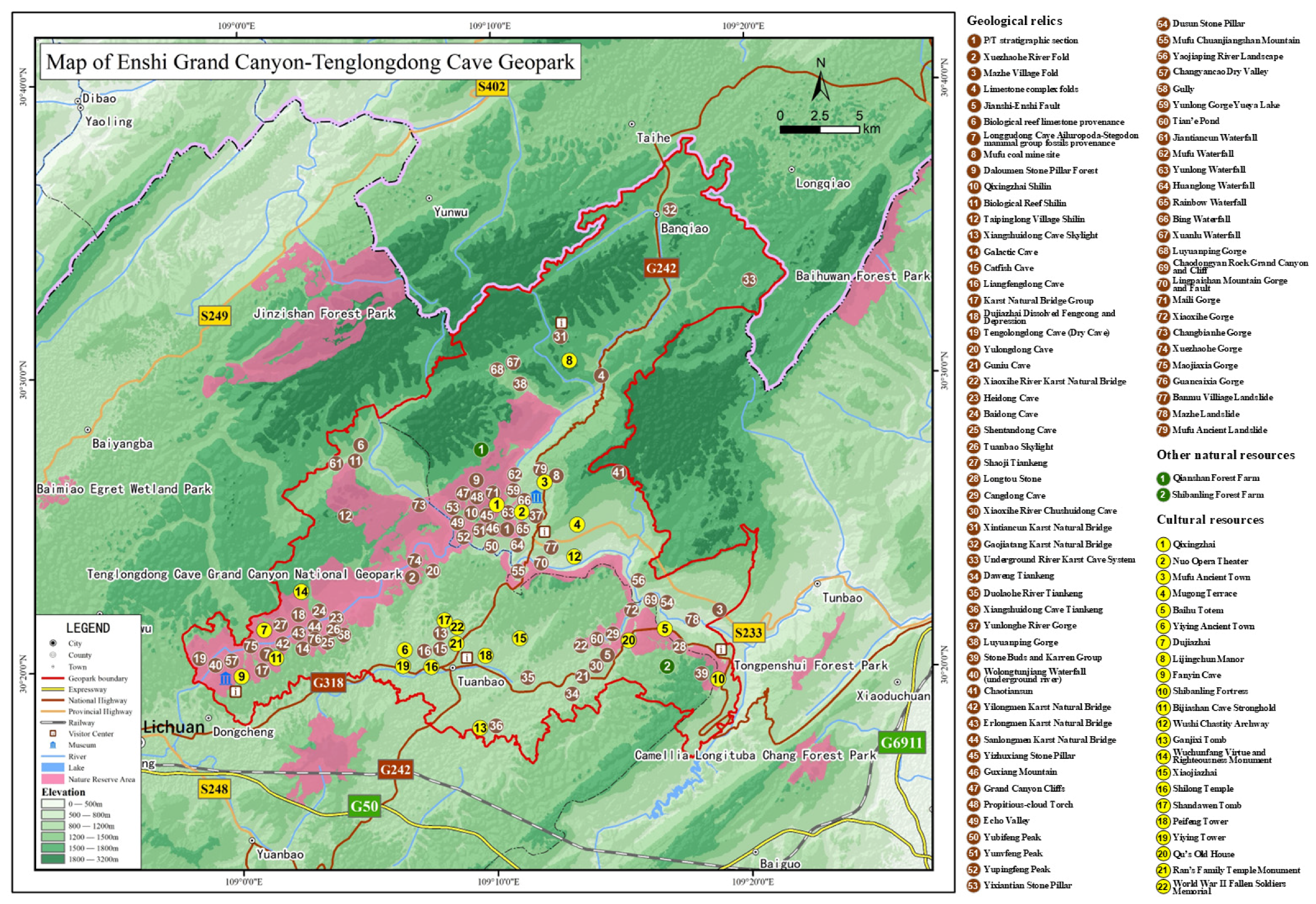
The Enshi Grand Canyon–Tenglongdong Cave UNESCO Global Geopark was selected as the study area due to its dual role as both an ecological conservation zone and a rapidly developing tourism destination, particularly since the opening of railway transport in 2010. The geopark exhibits marked spatial heterogeneity in land use, ranging from pristine karst forests to zones increasingly influenced by tourism infrastructure. This makes it an ideal setting for examining how natural and anthropogenic factors jointly shape ES dynamics. Insights from this case are expected to inform sustainable development strategies for other geoparks and fragile karst systems facing similar ecological and socio-economic challenges. As shown in Figure 2, the geopark hosts a rich concentration of geological heritage and other natural resources.

2.2. Data

This study comprehensively considered three types of driving factors: natural, socio-economic, and tourism. The natural factors included indicators such as soil type, terrain (elevation, slope, aspect), climate (temperature, precipitation), and vegetation coverage (NDVI) to reflect the background conditions of the ecosystem. The socio-economic factors were characterized by population density, GDP per capita, and land use changes to represent the intensity and mode of human activities. The tourism factors were measured by spatial accessibility indicators such as distance to roads, attractions, hotels, and residential areas to assess the pressure of tourism development. These indicators collectively formed a multidimensional dataset for analyzing the driving mechanisms of ecosystem services (Table 1).
The method for analyzing the interaction between raster data and tourism factors mainly involves spatialization processing: Firstly, non-grid data is converted into a grid layer with spatial continuity. Then, normalization processing is carried out: to eliminate the influence of scale, the Z-score normalization method is applied to each grid layer of the tourism element. Finally, resampling is performed to ensure that the spatial resolution of each layer is consistent with the basic geographic grid data. For each grid cell within the study area, this model not only incorporates the data values of natural and socio-economic rasters but also includes the specific distance between it and each tourism feature. This approach enables the model to quantify spatial distance and the pressure from tourism infrastructure, as well as how they combine with other driving factors to affect the local ESs at that specific location.
The selection of the four indicators of tourism factors—“distance from tourist attractions, distance from hotels, distance from roads, and distance from residential areas”—is mainly based on the following considerations: both theoretical representativeness and measurability. These four types of indicators can, respectively, represent the four key spatial dimensions of tourism development: core attractions (attractions), reception facilities (hotels), transportation accessibility (roads), and human settlement impact (residential areas). They jointly depict the main characteristics of the tourism spatial layout and its influence intensity and can all be accurately extracted from an open geographic data platform (OpenStreetMap), ensuring consistency across different periods. Regarding data availability and time consistency, during the research period (2010 to 2020), there was a lack of continuous and reliable social economic data such as tourist flow and ticket revenue. However, tourism facility data based on spatial location can be obtained through multi-period remote sensing and point-of-interest information, which can effectively reflect the spatial expansion process of tourism development.

2.3. Methods

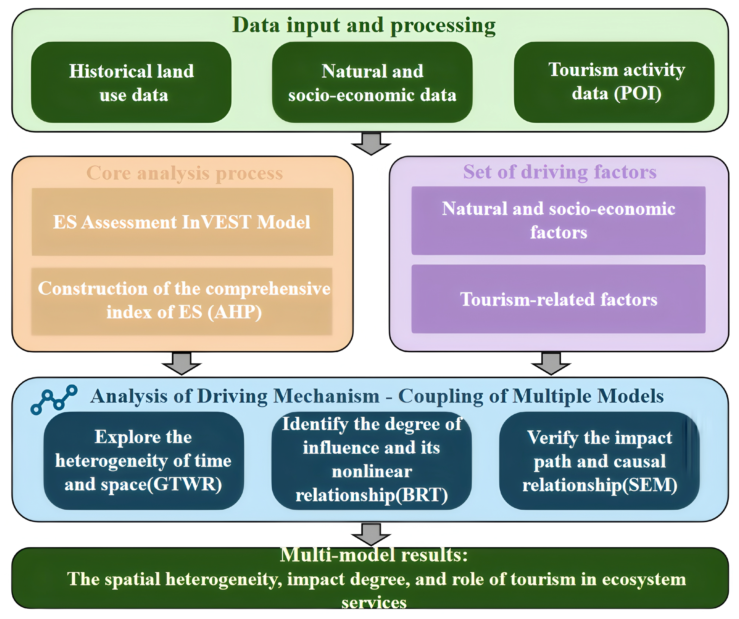
The analytical framework for this study was structured around three primary components. First, ESs and their spatiotemporal dynamics within the study area from 2010 to 2020 were quantified using the InVEST model and GTWR (for detailed data outputs, see Tables S1–S6 [28,29,30,31]). Second, the pathways through which various driving factors influence ESs were investigated by applying BRT and SEM (for detailed data outputs, see Tables S7 and S8). Finally, the impacts of tourism-related factors on ESs were assessed using the BRT model, providing a basis for formulating spatial planning strategies and management recommendations for the geopark (for detailed data outputs, see Table S9) (Figure 3).

2.3.1. ES Evaluations

To address the intricate interactions between humans and ecosystems, four key ESs—soil retention, water yield, carbon storage, and habitat quality—were quantitatively assessed using the InVEST 3.15.0 (Table 2).
The selection of these four environmental service indicators was specifically made based on the unique ecological characteristics and major environmental challenges of the karst region. The karst landscape, due to its rich biodiversity and unique hydrological system, is recognized worldwide. However, at the same time, due to its thin soil layer, high rock layer permeability, and slow soil formation rate, it is also one of the most ecologically fragile ecosystems in the world [38]. In this context, the following observations can be made: (1) Soil retention is a crucial regulating service. Severe soil erosion can lead to the rapid and irreversible degradation of the land, resulting in rock desertification [39]. (2) Water resource output capacity reflects the complex surface–underground dual hydrological structure, which is crucial for maintaining the ecological functions and water security of human use in the karst region [40]. (3) Carbon storage is particularly important because the karst ecosystem, due to its unique vegetation and soil processes, constitutes an important carbon sink, but it is highly susceptible to the impact of land use changes [41]. (4) Habitat quality directly reflects the ability of this ecosystem to support high species endemism and biodiversity levels in the karst terrain, and this biodiversity is highly vulnerable to the fragmentation of habitats caused by human activities [35]. Therefore, this set of ecological services provides a comprehensive and representative assessment of the core ecological assets and vulnerabilities within the studied karst geological park.

2.3.2. Comprehensive ES Index Assessment

The Analytic Hierarchy Process (AHP) was employed to develop a composite ecosystem service index (ESI) to avoid biases inherent in single-indicator assessments and to integrate the four key ecosystem service types. This multi-criteria decision-making method simplifies complex systems by structuring indicators into a hierarchical framework, transforming subjective expert knowledge into objective weights through systematic pairwise comparisons. A hierarchical model was established with the comprehensive ES assessment as the goal and the four ES indicators (soil conservation, carbon storage, water yield, and habitat quality) as the criteria level. Using yaahp 12.7, pairwise comparison matrices were constructed based on a 9-point intensity scale (Table 3) to determine the relative weights of each ES indicator [42,43]. The resulting composite ESI effectively captures both the ecological significance and practical relevance of these multidimensional ES indicators, providing a balanced representation of ESs for subsequent analysis.
To ensure the logical reliability of the pairwise comparisons, a consistency check was performed on each judgment matrix. The Consistency Index (CI) and Consistency Ratio (CR) were calculated as follows:
C I = λ m a x n n 1
C R = C I R I
where λmax is the principal eigenvalue of the judgment matrix, n is the number of indicators, and RI is the random index. A matrix was deemed consistent and its results acceptable only if the CR value was less than 0.10.
For judgment matrices that passed the consistency test, the normalized principal eigenvector corresponding to the maximum eigenvalue (λmax) was computed. This normalized eigenvector represents the final weight (wi) assigned to each indicator, reflecting its relative priority within the overall hierarchy. The final composite ESI was computed using the weighted sum method:
E S I = i = 1 n   ( w i I i )
where wi is the weight of the i-th indicator, and Ii is its standardized value. The ESI was subsequently mapped to visualize its spatial distribution across the study area for further analysis.

2.3.3. Identification of Influencing Factors Using GTWR

The Geographically and Temporally Weighted Regression (GTWR) model was applied to capture the spatiotemporal nonstationarity in relationships between driving factors and ESs. Unlike global regression approaches, GTWR allows regression coefficients to vary geographically and temporally, thereby effectively revealing the spatiotemporal heterogeneity of influencing mechanisms. The model was implemented in ArcGIS 10.8 with a spatiotemporal distance ratio of 1, and the optimal bandwidth was determined using the Akaike Information Criterion corrected (AICc) to ensure model precision. Local regression coefficients derived from the GTWR analysis were utilized to identify spatial variations in the direction and magnitude of influencing factors [44,45]. The model structure follows the following expression:
Y i = β 0 ( u i , v i , t i ) + k = 1 p   β k ( u i , v i , t i ) X i k + ε i
In this formula, (ui, vi, ti) represents the spatiotemporal coordinates of the i-th sample unit; Xik and Yi denote the explanatory variable and the explained variable, respectively; p is the number of explanatory variables; β0 (ui, vi, ti) is the intercept term; βk (ui, vi, ti) is the estimated coefficient of the k-th explanatory variable; and εi is the model residual. In addition, the bandwidth is optimally set using AICc, and the ratio of spatiotemporal distance parameters is 1.

2.3.4. Impacts of Influencing Factors on ESs

Structural equation modeling (SEM) was applied to elucidate causal pathways and validate the hypothesized “tourism–LUCC–ES” framework. This multivariate technique tests causal networks through measurement and structural models, moving beyond correlation to quantify direct and indirect effects. In this study, SEM was specifically used to verify whether tourism development influences ESs primarily by triggering land use/cover change and to decompose the magnitude of these mediated effects, thereby providing mechanistic insights into ecosystem service dynamics [46].
Boosted Regression Tree (BRT) modeling was employed to capture nonlinear responses and threshold effects in tourism–ES relationships. As a machine learning ensemble technique, BRT iteratively fits decision trees to model complex patterns [47]. The model served to identify critical thresholds in tourism disturbance factors and quantify the relative importance of each driver, complementing SEM by revealing nonlinear dynamics that traditional linear models might overlook.

3. Results

3.1. Comprehensive Ecosystem Service Index Assessment and Spatiotemporal Changes

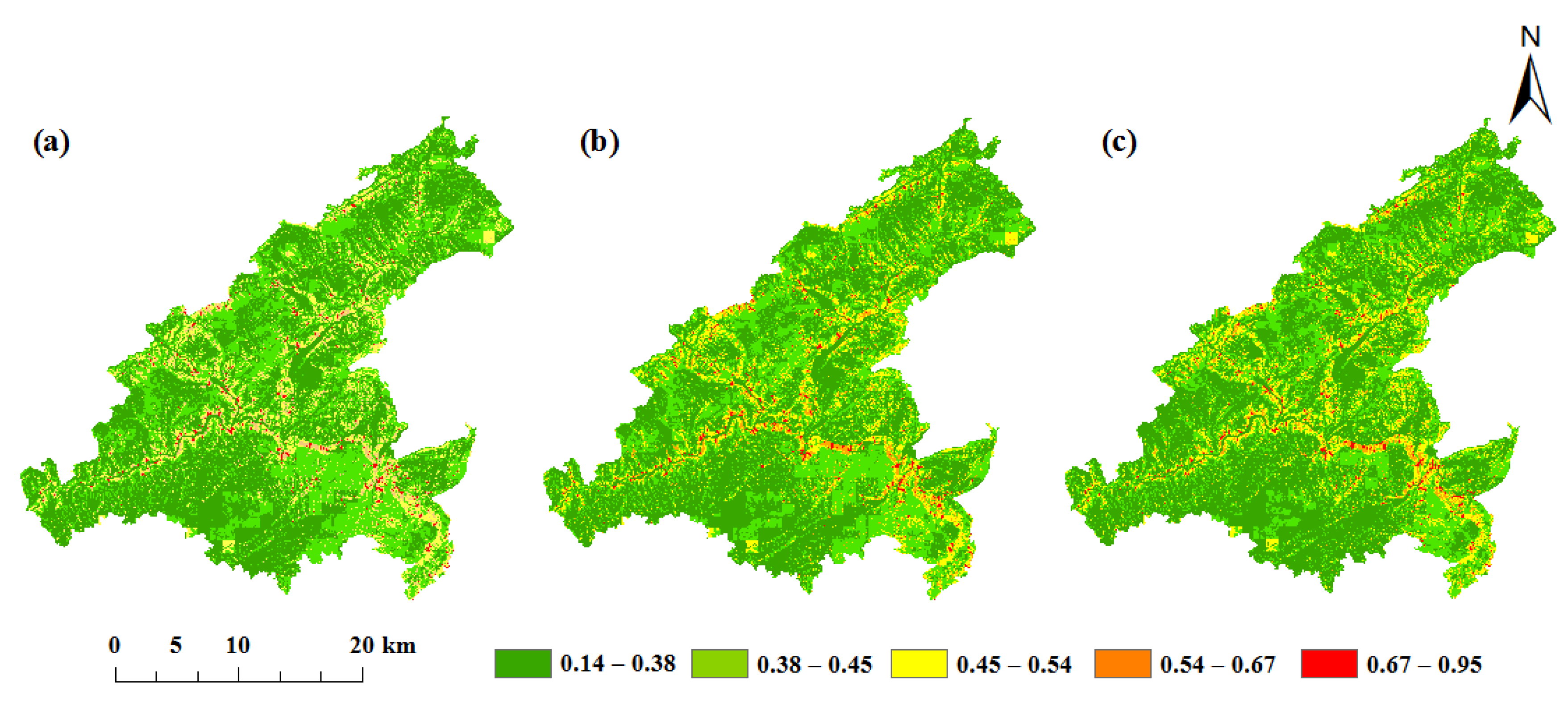
The comprehensive ecosystem service index (ESI) indicates that from 2010 to 2020, the overall ecosystem services showed a slight downward trend, and this trend was uneven across different regions. It manifested as the continuous expansion of low-service-level areas, especially in the northern part of the study area. Although some local improvements were observed—that is, the medium-level service areas transformed into higher-level areas—these scattered improvements were not sufficient to counteract the overall downward trend. Throughout the entire study period, the high-value ecosystem service areas remained scattered and fragmented, and no substantial integration or spatial expansion occurred in these critical ecological areas (Figure 4).

3.2. Driving Forces of Changes in ESs

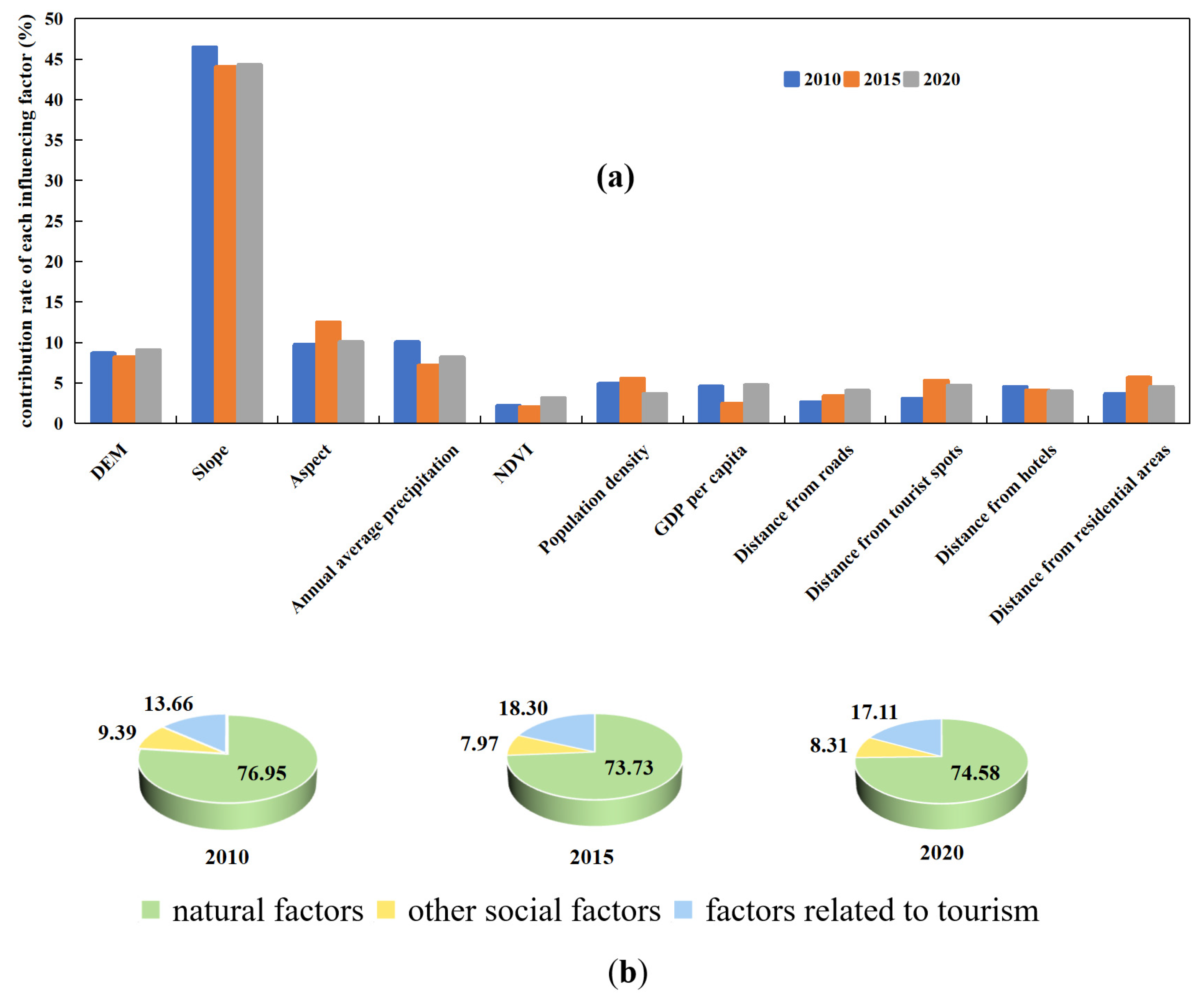
The GTWR model demonstrated superior performance over the global ordinary least squares (OLS) approach in capturing the spatiotemporal heterogeneity of driving mechanisms (Table 4). Three key patterns were identified in the factor contributions: (1) Natural factors consistently dominated ES dynamics (>73% total contribution), though tourism factors showed a gradually increasing influence. (2) Slope persistently served as the key determinant, while other topographic factors like the DEM exhibited fluctuating contributions (Figure 5a). (3) Tourism-related factors displayed substantial interannual variability in their contribution rates, indicating phase-specific impacts on ESs (Figure 5b). These findings collectively reveal the complex, nonstationary nature of tourism–ES interactions across space and time.
Among all the factors that affect the ecosystem, slope consistently demonstrates a high contribution ratio, thereby confirming its role as a key determinant. In contrast, basic topographic factors (such as the DEM) show a dynamic but relatively stable pattern of influence throughout the entire study period. Factors such as aspect and precipitation, however, exhibit more significant fluctuations in their relative influence levels—reflecting their higher sensitivity to interannual climate changes. Figure 5a presents the statistical values of the key factors. Individual explanatory factors with lower individual explanatory power will be discussed in the context of interaction effects. Overall, natural factors are recognized as the dominant category, contributing more than 73% to the total ecosystem contribution rate during the period from 2010 to 2020. In comparison, factors related to tourism constitute the second most important influencing category, while the contributions of other socio-economic factors are the lowest. It is notable that the contributions of factors related to tourism show significant interannual variations throughout the study period (Figure 5b).

3.3. Spatial Heterogeneity of Tourism Impacts

The cross-validation results of the Boosted Regression Tree (BRT) model (Table 5) revealed a highly significant positive correlation (p < 0.001) between ESs and both the observed and fitted values of the influencing factors across all study years. The Root Mean Square Error (RMSE) values consistently approached zero, demonstrating a good model fit and confirming the reliability of the simulation outcomes.
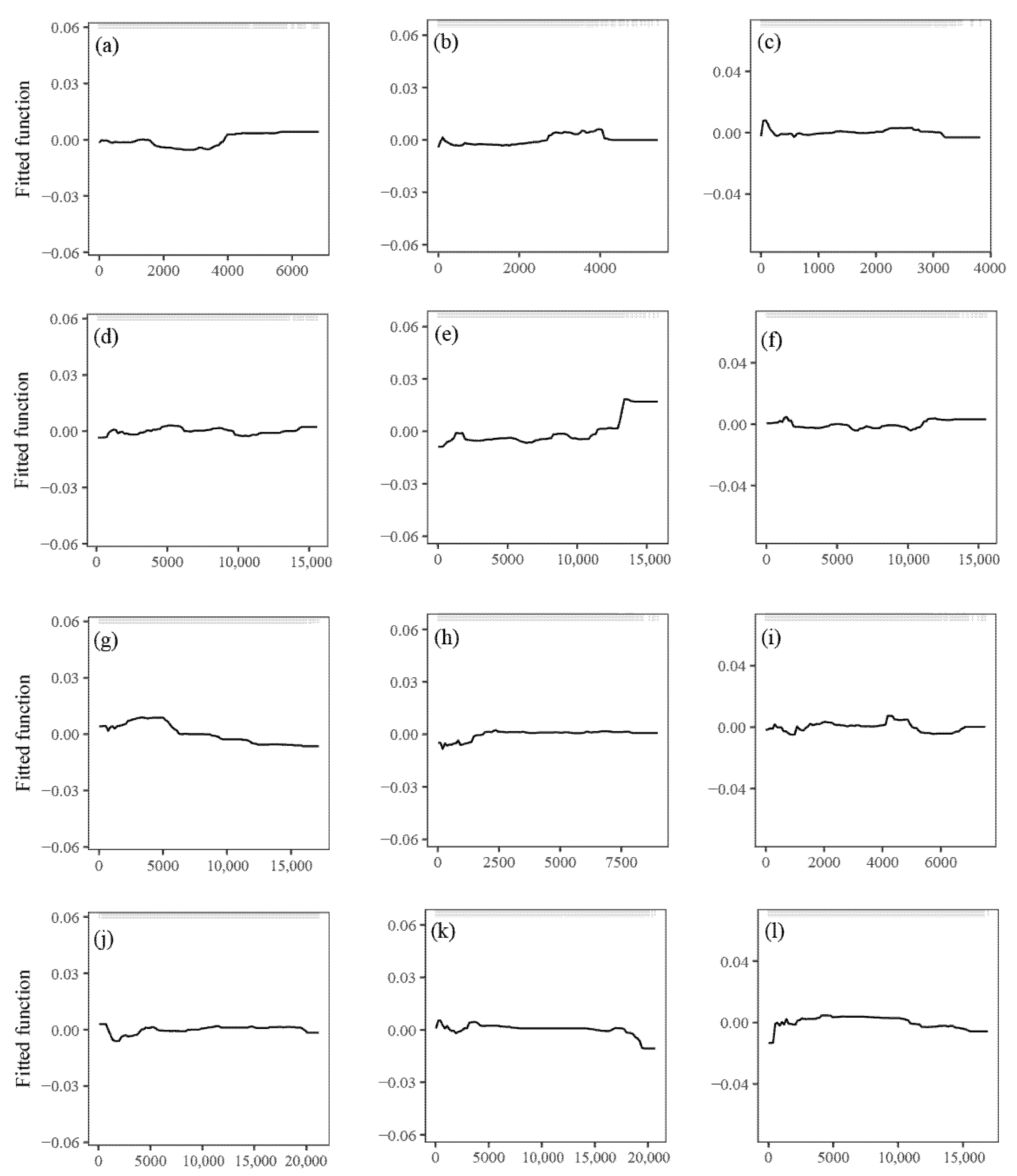
The Boosted Regression Tree (BRT) model effectively captured the nonlinear relationships and threshold effects between tourism factors and ESs, revealing four distinct spatial patterns (Figure 6). (1) Proximity to scenic spots exhibited persistently negative effects that expanded spatially over time, indicating a growing ecological pressure from tourism concentration. (2) The influence of hotel proximity transitioned from negative to positive, suggesting potential benefits from improved management practices and infrastructure development. (3) Road access maintained generally positive effects on ESs, though these became more localized in later study periods. (4) Residential areas consistently showed negative impacts, with intensity diminishing with increasing distance. The BRT model’s ability to identify these complex nonlinear responses highlights its advantage over traditional linear models in capturing the threshold behaviors and spatial heterogeneity of tourism–ES interactions.
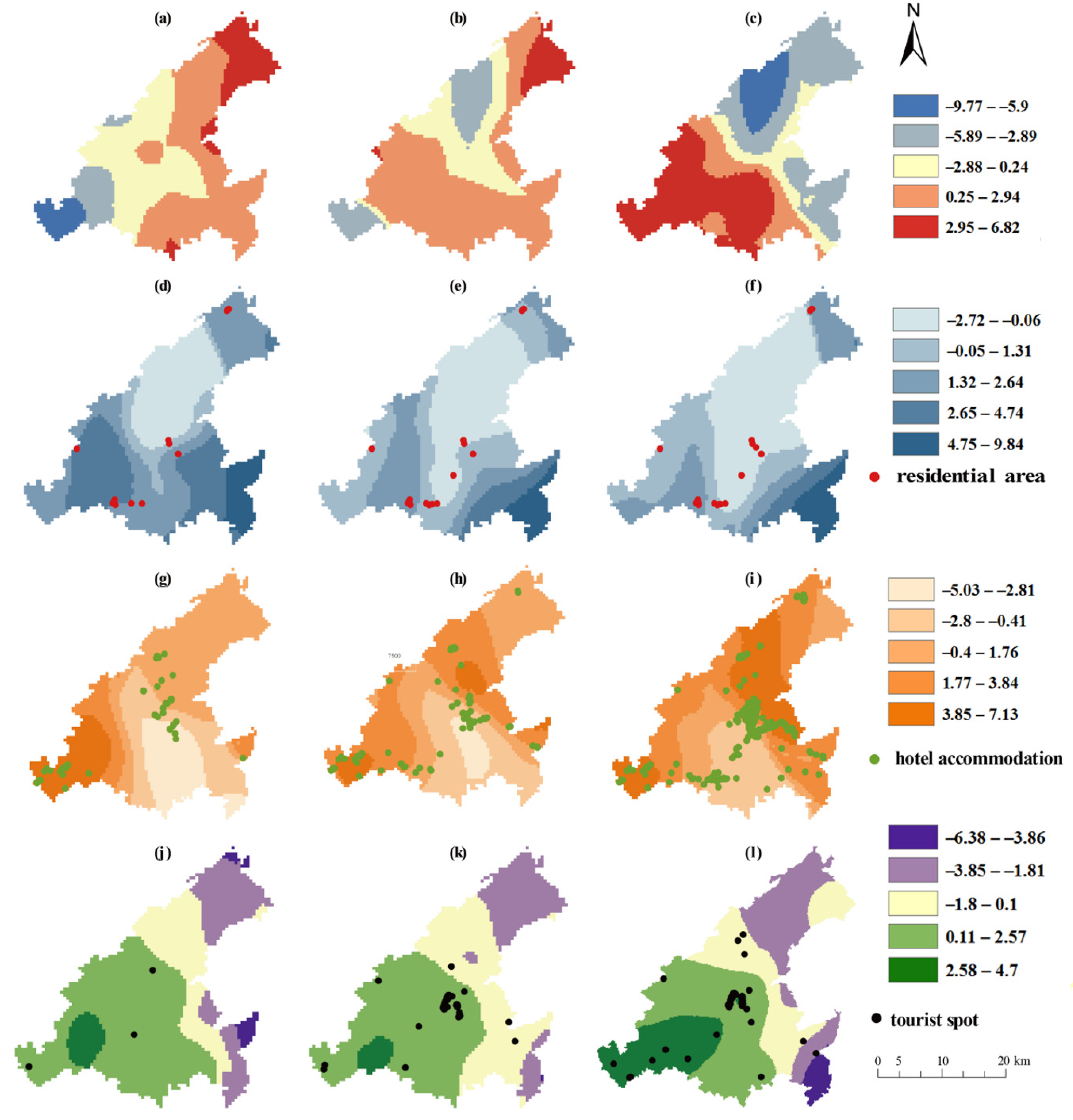
The spatiotemporally heterogeneous impacts of tourism factors on ecosystem services (ESs) were elucidated by the Geographically and Temporally Weighted Regression (GTWR) model (Figure 7). Analysis of Figure 7a–c confirms the generally positive influence of road access, while revealing its increasingly localized nature over time. Figure 7d–f visualizes a clear distance-decay gradient for the negative effects of residential areas. Notably, the influence of hotel proximity (Figure 7g–i) transitioned complexly, with coexisting negative and positive clusters, explaining its aggregate nonlinear effect. Most critically, the persistently negative impact of scenic spots intensified and its spatial footprint expanded markedly from 2010 to 2020 (Figure 7j–l), signaling escalating ecological pressure from tourism concentration. The GTWR model’s ability to uncover these complex, non-stationary dynamics highlights its superiority over traditional linear approaches for dissecting tourism-ES interactions.

3.4. Driving Pathways of Tourism Factors on ESs

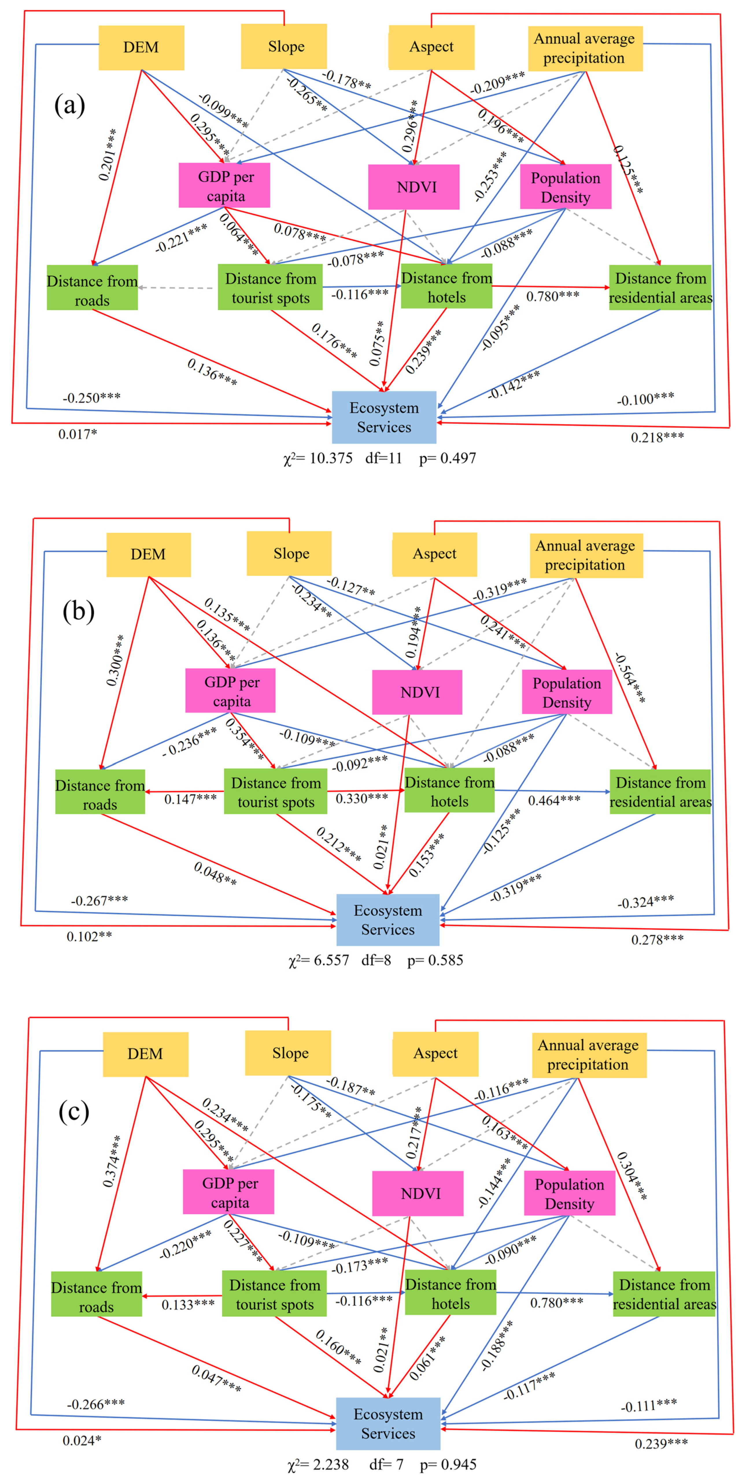
SEM was employed to elucidate the complex causal pathways through which tourism factors influence ESs, with land use/cover change (LUCC) identified as the critical mediating mechanism. The analysis revealed distinct evolutionary patterns across three developmental phases, demonstrating how tourism–ES interactions transformed over the decade (Figure 8).
During the initial development phase (2010), infrastructure proximity exhibited strong positive effects on ESs, with distance to hotels (β = 0.239), residential areas (β = 0.176), and roads (β = 0.136) all showing significant positive correlations. In contrast, proximity to scenic spots demonstrated negative effects (β = −0.142), indicating the contrasting roles of tourism infrastructure versus core attractions in ES provision.
The rapid expansion phase (2015) witnessed significant transformations, with the negative effect of scenic spot proximity intensifying substantially (β = −0.319), reflecting escalating ecological pressure from tourism concentration. While residential distance maintained positive effects (β = 0.212), potentially indicating environmental management improvements, the benefits of road and hotel proximity diminished, suggesting saturation effects in infrastructure development.
In the mature phase (2020), the influence magnitudes of all tourism factors generally weakened, with scenic spot effects reducing to β = −0.117 and infrastructure effects showing further decline. Most significantly, SEM quantification revealed that tourism development primarily affects ESs indirectly through triggering LUCC, which explains approximately 65% of the total effect. This central finding establishes LUCC as the dominant pathway in tourism–ecosystem interactions and provides mechanistic understanding for sustainable landscape planning in ecologically sensitive regions.

4. Discussion

4.1. The Dual Effects of Tourism on ESs

This study demonstrates that tourism exerts spatially and temporally heterogeneous impacts on ESs, characterized by a distinct duality of positive and negative effects. The positive influences primarily stem from improved ecological management, infrastructure development, and the reinvestment of tourism revenues into environmental protection initiatives. In contrast, intensive tourism activities concentrated in core scenic areas have led to pronounced ecological degradation, including vegetation loss, soil erosion, and habitat fragmentation. Comparable patterns have been reported globally—for example, in European and North American national parks where tourism revenue has been successfully reinvested in conservation programs [48,49,50], as well as in overdeveloped coastal regions of Southeast Asia and the Mediterranean, where excessive tourism has accelerated environmental degradation [51,52,53].
Our research adopted a comprehensive modeling approach, aiming to go beyond simple correlation analysis and reveal the complex direct and indirect pathways through which natural, socio-economic, and tourism factors affect ecosystem services (ESs). The results of the structural equation model (SEM) provided strong empirical verification for the indirect influence path of “tourism → urbanization and land use change → ecosystem services”, which accounted for approximately 65% of the total tourism effect. This finding is crucial as it clarifies that the main ecological footprint of tourism is not the immediate presence of tourists but the land transformation it triggers. This mechanistic understanding was further analyzed through the regression tree (BRT) model, which quantified the relative influence of each driving factor. The results showed that natural factors (totaling over 73%) always remained the dominant force shaping the ecosystem service pattern, and this remained the case throughout the study period.
The BRT analysis offers nuanced insights into key determinants. Slope consistently emerged as a pivotal factor, corroborating its established role in karst ecosystems globally [54]. Steeper slopes in our study area are associated with thinner soils and higher susceptibility to erosion, which naturally constrains human development and agriculture, thereby preserving high-quality forest habitats and their associated ESs (e.g., soil retention, carbon sequestration). This finding aligns with studies in the Wuling Mountains and other karst regions where slope has been a primary determinant of habitat quality and soil erosion risk [55]. However, our study adds a novel dimension by demonstrating that tourism’s impact intensified over time and exhibited significant spatial heterogeneity, as captured by the GTWR model. The negative impacts were the most acute in areas of high tourism concentration, where the natural protective effect of steep slopes was overridden by the direct physical footprint of infrastructure.
However, over time, this relationship weakened and even reversed in some zones, as seen in the SEM and GTWR results. We postulate that this transition reflects the implementation of localized environmental management measures, such as the concentration of infrastructure to minimize sprawl and investments in green infrastructure within hotel zones, effectively demonstrating the potential for adaptive management to decouple tourism infrastructure from ecological impact. Moreover, the transition of hotel-related impacts—from initially negative to increasingly positive during the study period—demonstrates the potential reversibility of tourism-induced ecological effects [56]. This spatial-targeted approach aligns with the principle of identifying synergistic priorities for conservation, as demonstrated on the Qinghai-Tibetan Plateau [57], and effectively demonstrates the potential for adaptive management to decouple tourism infrastructure from ecological impact. This finding underscores that adverse tourism impacts can be mitigated through adaptive management strategies, which are essential for navigating the complex spatial interplay between urbanization and ecosystem services, as highlighted in large basin studies [58], including the following:
(1)
Spatially differentiated measures such as zoning control and restrictions on development within core scenic areas;
(2)
Restorative interventions including vegetation recovery around hotel zones and the rehabilitation of degraded land;
(3)
The reinvestment of tourism-generated revenue into conservation programs to ensure long-term ecological sustainability.

4.2. Research Shortcomings and Limitations

Several methodological limitations of this study should be acknowledged to inform future research directions. First, constraints in remote sensing spatial resolution and the temporal granularity of POI data may have restricted the detection of short-term tourism disturbances and fine-scale ecological responses. Second, although the integrated modeling framework (GTWR–BRT–SEM) substantially improved the mechanistic understanding of tourism–ecosystem interactions compared to traditional approaches, key social dimensions—such as tourist mobility, consumption behavior, and spatial flow patterns—were not incorporated into the analytical structure. Third, as this research focuses on a single karst geopark ecosystem, the generalizability of its findings requires further validation across other ecological contexts, including coastal, desert, and alpine environments. Nevertheless, the proposed methodological framework possesses strong transferability and can be adapted for application in other ecologically fragile systems.
Future research should therefore prioritize the integration of higher-resolution temporal datasets and emerging multi-source information, such as social media analytics, mobile phone signaling data, and high-frequency satellite imagery, to better capture rapid ecological responses to tourism pressures. Additionally, constructing more comprehensive modeling frameworks that explicitly account for tourist behavior dynamics, policy interventions, and cross-boundary ecological processes would greatly enhance the understanding of the complex feedback mechanisms linking tourism and ESs. Such efforts will provide a stronger theoretical foundation for advancing sustainable tourism management across diverse ecological regions.

5. Conclusions

This study elucidated the complex interactions between tourism development and ESs in ecologically sensitive geoparks. Three principal conclusions were drawn:
(1)
Natural factors remain the dominant determinants of ES patterns; however, the influence of tourism has shown a clear and accelerating upward trend.
(2)
Tourism impacts exhibit pronounced spatiotemporal heterogeneity—persistent negative effects coexist with emerging positive outcomes across different landscape elements.
(3)
The primary mechanism through which tourism affects ESs operates indirectly via LUCC, thereby empirically validating and extending the theoretical “tourism–LUCC–ES” framework.
Methodologically, this research demonstrates the robustness of the integrated multi-model framework in systematically assessing complex human–environment interactions. Theoretically, it advances the understanding of the indirect pathways and feedback processes linking tourism activities to ecological outcomes. In practice, our research results are directly relevant to the management of the Enshi Grand Canyon Global Geopark. They have been adopted by the park’s administration, providing practical and feasible insights for the sustainable development of tourism in the area, which have been transformed into three key management recommendations:
(1)
Implement spatial zoning strategies that strictly regulate construction in core scenic areas while promoting ecological restoration in degraded zones;
(2)
Establish an ecological compensation mechanism financed by tourism enterprises to support land rehabilitation;
(3)
Develop a multi-scale ecological monitoring and early warning system combining remote sensing data and on-site ecological indicators to identify the critical thresholds of ecosystem degradation.

Supplementary Materials

The following supporting information can be downloaded at: https://www.mdpi.com/article/10.3390/land14112262/s1. References [55,56,57,58] are cited in the Supplementary Materials file.

Author Contributions

Conceptualization, J.P. and J.L.; Data curation, J.P., Y.Z. and X.X.; Investigation, J.P. and J.L.; Methodology, J.P. and J.L.; Resources, J.P., Y.Z., J.L. and X.X.; Writing—original draft, J.P.; Writing—review and editing, J.P. and J.L. All authors have read and agreed to the published version of the manuscript.

Funding

This research was funded by the Ecological Culture Tourism Research Center of Western Hubei province and the National Key Research Base on Rural Poverty in Contiguous Poverty-stricken Areas (Wuling Mountain Area) of China, grant number PT072109.

Data Availability Statement

The data presented in this study are available on request from the corresponding author.

Acknowledgments

The authors sincerely thank all the experts for their contributions to data collection, model construction, and strategy formulation in this research. All the individuals mentioned here have agreed to accept this acknowledgement. We are grateful to the anonymous reviewers for their valuable comments and suggestions.

Conflicts of Interest

The authors declare no conflicts of interest.

Abbreviations

The following abbreviations are used in this manuscript:
ESsEcosystem Services
UNESCOUnited Nations Educational, Scientific, and Cultural Organization
POIsPoints of Interest
InVESTIntegrated Valuation of Ecosystem Services and Tradeoffs
GTWRGeographically and Temporally Weighted Regression
BRTsBoosted Regression Trees
SEMStructural Equation Modeling
LUCCLand Use and Land Cover Change

References

  1. Ouyang, Z.; Zheng, H.; Xiao, Y.; Polasky, S.; Liu, J.; Xu, W.; Wang, Q.; Zhang, L.; Xiao, Y.; Rao, E.; et al. Improvements in ecosystem services from investments in natural capital. Science 2016, 352, 1455–1459. [Google Scholar] [CrossRef]
  2. Xue, H.; Li, S.; Chang, J. Combining ecosystem service relationships and DPSIR framework to manage multiple ecosystem services. Environ. Monit. Assess. 2015, 187, 117. [Google Scholar] [CrossRef]
  3. Xiong, S.; Yang, F.; Zhang, J.; Li, J.; Gu, C. Advancing multiscale sustainable development in lake-dense regions: A dynamic management chain for ecosystem service supply-demand and ecological risks interactions. J. Environ. Manag. 2025, 386, 125737. [Google Scholar] [CrossRef] [PubMed]
  4. Kubiszewski, I.; Costanza, R.; Anderson, S.; Sutton, P. The future value of ecosystem services: Global scenarios and national implications. Ecosyst. Serv. 2017, 26, 289–301. [Google Scholar] [CrossRef]
  5. Melese, W. Ecosystem Services and Tourism Potential in Lake Tana Peninsula: Ethiopia Review. J. Tour. Hosp. 2017, 6, 1–6. [Google Scholar]
  6. Costanza, R.; Kubiszewski, I.; Rasheed, R. Commentary: The Future of Changes in Global Ecosystem Services. Glob. Environ. Change-Hum. Policy Dimens. 2021, 71, 102399. [Google Scholar] [CrossRef]
  7. Costanza, R.; Farber, S. Introduction to the special issue on the dynamics and value of ecosystem services: Integrating economic and ecological perspectives. Ecol. Econ. 2002, 41, 367–373. [Google Scholar] [CrossRef]
  8. Andrew, C.; Tim, C.; Rob, F. Tourism in sub-global assessments of ecosystem services. J. Sustain. Tour. 2017, 25, 1529–1546. [Google Scholar] [CrossRef]
  9. Jasper, H.H.; Peter, G.; Frank, V. Using a social-ecological systems perspective to understand tourism and landscape interactions in coastal areas. J. Tour. Futures 2017, 3, 23–38. [Google Scholar]
  10. Shao, Y.; Xiao, Y.; Sang, W. Land use trade-offs and synergies based on temporal and spatial patterns of ecosystem services in South China. Ecol. Indic. 2022, 143, 109335. [Google Scholar] [CrossRef]
  11. Zeng, Y.; Zhong, L.; Wang, L. Spatiotemporal changes in recreation potential of ecosystem services in Sanjiangyuan, China. J. Spat. Sci. 2018, 63, 359–377. [Google Scholar] [CrossRef]
  12. Mita, D.; Lucia, B.; Daniel, D.; Menegon, S.; Pugnetti, A.; Stifter, S. Tackling challenges for Mediterranean sustainable coastal tourism: An ecosystem service perspective. Sci. Total Environ. 2018, 652, 1302–1317. [Google Scholar]
  13. Turner, K.G.; Anderson, S.; Gonzalez-Chang, M.; Costanza, R.; Courville, S.; Dalgaard, T.; Dominati, E.; Kubiszewski, I.; Ogilvy, S.; Porfirio, L.; et al. A review of methods, data, and models to assess changes in the value of ecosystem services from land degradation and restoration. Ecol. Model. 2016, 319, 190–207. [Google Scholar] [CrossRef]
  14. Zhou, Z.; Liu, X.; Zheng, B.; Robinson, G.M.; Song, B. Agricultural Transformation and Its Impact on Ecosystem Services and Human Well-Being in Peri-Urban Areas: The Case of Xi’an, China. Land 2022, 11, 110. [Google Scholar] [CrossRef]
  15. Li, Y.; Luo, Y.; Liu, G.; Ouyang, Z.; Zheng, H. Effects of land use change on ecosystem services: A case study in Miyun reservoir watershed. Acta Ecol. Sin. 2013, 33, 726–736. [Google Scholar] [CrossRef]
  16. Yuan, R.; Zhang, N.; Zhang, Q. The impact of habitat loss and fragmentation on biodiversity in global protected areas. Sci. Total Environ. 2024, 931, 173004. [Google Scholar] [CrossRef]
  17. Chiappero, M.F.; Rossetti, M.R.; Moreno, M.L.; Pérez-Harguindeguy, N. A global meta-analysis reveals a consistent reduction of soil fauna abundance and richness as a consequence of land use conversion. Sci. Total Environ. 2024, 946, 173822. [Google Scholar] [CrossRef]
  18. Lü, Y.; Ma, Z.; Zhao, Z.; Sun, F.; Fu, B. Effects of land use change on soil carbon storage and water consumption in an oasis-desert ecotone. Environ. Manag. 2014, 53, 1066–1076. [Google Scholar] [CrossRef]
  19. Yang, W.; Schmidt, C.; Wu, S.; Zhao, Z.; Li, R.; Wang, Z.; Wang, H.; Hua, P.; Krebs, P.; Zhang, J. Exacerbated anthropogenic water pollution under climate change and urbanization. Water Res. 2025, 280, 123449. [Google Scholar] [CrossRef] [PubMed]
  20. Hanna, D.E.; Raudsepp-Hearne, C.; Bennett, E.M. Effects of land use, cover, and protection on stream and riparian ecosystem services and biodiversity. Conserv. Biol. 2020, 34, 244–255. [Google Scholar] [CrossRef]
  21. Chi, W.; Zhao, Y.; Kuang, W.; He, H. Impacts of anthropogenic land use/cover changes on soil wind erosion in China. Sci. Total Environ. 2019, 668, 204–215. [Google Scholar] [CrossRef]
  22. Spake, R.; Lasseur, R.; Crouzat, E.; Bullock, J.M.; Lavorel, S.; Parks, K.E.; Schaafsma, M.; Bennett, E.M.; Maes, J.; Mulligan, M.; et al. Unpacking ecosystem service bundles: Towards predictive mapping of synergies and trade-offs between ecosystem services. Glob. Environ. Change-Hum. Policy Dimens. 2017, 47, 37–50. [Google Scholar] [CrossRef]
  23. Locatelli, B.; Imbach, P.; Wunder, S. Synergies and trade-offs between ecosystem services in Costa Rica. Environ. Conserv. 2014, 41, 27–36. [Google Scholar] [CrossRef]
  24. Bradford, J.B. Potential Influence of Forest Management on Regional Carbon Stocks: An Assessment of Alternative Scenarios in the Northern Lake States, USA. For. Sci. 2011, 57, 479–488. [Google Scholar] [CrossRef]
  25. McNally, C.G.; Uchida, E.; Gold, A.J. The effect of a protected area on the tradeoffs between short-run and long-run benefits from mangrove ecosystems. Proc. Natl. Acad. Sci. USA 2011, 108, 13945–13950. [Google Scholar] [CrossRef] [PubMed]
  26. Costanza, R.; Mitsch, W.; Day, J.W. A new vision for New Orleans and the Mississippi delta: Applying ecological economics and ecological engineering. Front. Ecol. Environ. 2006, 4, 465–472. [Google Scholar] [CrossRef]
  27. Li, Y.-J.; Ouyang, C.-X.; Zhou, S.-Y.; Yu, H.; Knight, W.D. Tourism dependence and poverty alleviation thresholds in Chinese ethnic tourism. J. Mt. Sci. 2022, 19, 3026–3036. [Google Scholar] [CrossRef]
  28. Wu, L.; Sun, C.; Fan, F. Estimating the Characteristic Spatiotemporal Variation in Habitat Quality Using the InVEST Model—A Case Study from Guangdong-Hong Kong-Macao Greater Bay Area. Remote Sens. 2021, 13, 1008. [Google Scholar] [CrossRef]
  29. Zhang, Y.; Pan, Y.; Li, M.; Wang, Z.; Wu, J.; Zhang, X.; Cao, Y. Impacts of human appropriation of net primary production on ecosystem regulating services in Tibet. Ecosyst. Serv. 2021, 47, 101231. [Google Scholar] [CrossRef]
  30. Li, Y.; Yao, S.; Jiang, H.; Wang, H.; Ran, Q.; Gao, X.; Ding, X.; Ge, D. Spatial-Temporal Evolution and Prediction of Carbon Storage: An Integrated Framework Based on the MOP-PLUS- InVEST Model and an Applied Case Study in Hangzhou, East China. Land 2022, 11, 2213. [Google Scholar] [CrossRef]
  31. Wu, J.; Jin, X.; Feng, Z.; Chen, T.; Wang, C.; Feng, D.; Lv, J. Relationship of Ecosystem Services in the Beijing-Tianjin-Hebei Region Based on the Production Possibility Frontier. Land 2021, 10, 881. [Google Scholar] [CrossRef]
  32. Gao, Y.; Song, Y.; Yang, L.; Hu, Y.; Hao, J.; Tian, J.; Li, Z. Revealing spatiotemporal heterogeneity of water conservation and its drivers: Enlightenment to water ecology protection and restoration. J. Environ. Manag. 2024, 370, 122517. [Google Scholar] [CrossRef]
  33. Li, Z.; Deng, X.; Jin, G.; Mohmmed, A.; Arowolo, A.O. Tradeoffs between agricultural production and ecosystem services: A case study in Zhangye, Northwest China. Sci. Total Environ. 2020, 707, 136032. [Google Scholar] [CrossRef]
  34. Adelisardou, F.; Jafari, H.R.; Malekmohammadi, B.; Minkina, T.; Zhao, W.; Karbassi, A. Impacts of land use and land cover change on the interactions among multiple soil-dependent ecosystem services (case study: Jiroft plain, Iran). Environ. Geochem. Health 2021, 43, 3977–3996. [Google Scholar] [CrossRef] [PubMed]
  35. Benez-Secanho, F.J.; Dwivedi, P. Analyzing the provision of ecosystem services by conservation easements and other protected and non-protected areas in the Upper Chattahoochee Watershed. Sci. Total Environ. 2020, 717, 137218. [Google Scholar] [CrossRef]
  36. He, Q.; Bertness, M.D.; Bruno, J.F.; Li, B.; Chen, G.; Coverdale, T.C.; Altieri, A.H.; Bai, J.; Sun, T.; Pennings, S.C.; et al. Economic development and coastal ecosystem change in China. Sci. Rep. 2014, 4, 5995. [Google Scholar] [CrossRef] [PubMed] [PubMed Central]
  37. Tian, Y.; Wang, S.; Bai, X.; Luo, G.; Xu, Y. Trade-offs among ecosystem services in a typical Karst watershed, SW China. Sci. Total Environ. 2016, 566, 1297–1308. [Google Scholar] [CrossRef]
  38. Wang, H.; Wang, W.J.; Liu, Z.; Wang, L.; Zhang, W.; Zou, Y.; Jiang, M. Combined effects of multi-land use decisions and climate change on water-related ecosystem services in Northeast China. J. Environ. Manag. 2022, 315, 115131. [Google Scholar] [CrossRef]
  39. Adelisardou, F.; Mederly, P.; Minkina, T. Assessment of soil- and water-related ecosystem services with coupling the factors of climate and land-use change (Example of the Nitra region, Slovakia). Environ. Geochem. Health 2023, 45, 6605–6620. [Google Scholar] [CrossRef]
  40. Deng, C.; Liu, J.; Liu, Y.; Li, Z.; Nie, X.; Hu, X.; Wang, L.; Zhang, Y.; Zhang, G.; Zhu, D.; et al. Spatiotemporal dislocation of urbanization and ecological construction increased the ecosystem service supply and demand imbalance. J. Environ. Manag. 2021, 288, 112478. [Google Scholar] [CrossRef] [PubMed]
  41. Seppelt, R.; Lautenbach, S.; Volk, M. Identifying trade-offs between ecosystem services, land use, and biodiversity: A plea for combining scenario analysis and optimization on different spatial scales. Curr. Opin. Environ. Sustain. 2013, 5, 458–463. [Google Scholar] [CrossRef]
  42. Das, B.; Desai, S.; Daripa, A.; Anand, G.C.; Kumar, U.; Khalkho, D.; Thangavel, V.; Kumar, N.; Reddy, G.P.O.; Kumar, P. Land degradation vulnerability mapping in a west coast river basin of India using analytical hierarchy process combined machine learning models. Environ. Sci. Pollut. Res. Int. 2023, 30, 83975–83990. [Google Scholar] [CrossRef]
  43. Bin, L.; Xu, K.; Pan, H.; Zhuang, Y.; Shen, R. Urban flood risk assessment characterizing the relationship among hazard, exposure, and vulnerability. Environ. Sci. Pollut. Res. Int. 2023, 30, 86463–86477. [Google Scholar] [CrossRef]
  44. Ding, Y.R.; Liu, X.; Dai, X.F.; Yang, Y.; Yin, G.Y.; Sun, H.P.; Guo, J.Y. Spatiotemporal analysis of sea ice in the Weddell Sea of Antarctic based on GTWR. Sci. Rep. 2025, 15, 5863. [Google Scholar] [CrossRef] [PubMed]
  45. Wang, H.; Zhao, M.; Huang, X.; Song, X.; Cai, B.; Tang, R.; Sun, J.; Han, Z.; Yang, J.; Liu, Y.; et al. Improving prediction of soil heavy metal(loid) concentration by developing a combined Co-kriging and geographically and temporally weighted regression (GTWR) model. J. Hazard. Mater. 2024, 468, 133745. [Google Scholar] [CrossRef] [PubMed]
  46. Li, J.; Auchincloss, A.H.; Yang, Y.; Rodriguez, D.A.; Sánchez, B.N. Neighborhood characteristics and transport walking: Exploring multiple pathways of influence using a structural equation modeling approach. J. Transp. Geogr. 2020, 85, 102703. [Google Scholar] [CrossRef]
  47. Cheong, Y.L.; Leitão, P.J.; Lakes, T. Assessment of land use factors associated with dengue cases in Malaysia using Boosted Regression Trees. Spat Spatiotemporal Epidemiol. 2014, 10, 75–84. [Google Scholar] [CrossRef]
  48. Lanzas, M.; Hermoso, V.; De-Miguel, S.; Bota, G.; Brotons, L. Designing a network of green infrastructure to enhance the conservation value of protected areas and maintain ecosystem services. Sci. Total Environ. 2019, 651 Pt 1, 541–550. [Google Scholar] [CrossRef] [PubMed]
  49. Pfueller, S.L.; Lee, D.; Laing, J. Tourism partnerships in protected areas: Exploring contributions to sustainability. Environ. Manag. 2011, 48, 734–749. [Google Scholar] [CrossRef]
  50. Carroll, C.; Ray, J.C. Maximizing the effectiveness of national commitments to protected area expansion for conserving biodiversity and ecosystem carbon under climate change. Glob. Chang. Biol. 2021, 27, 3395–3414. [Google Scholar] [CrossRef] [PubMed] [PubMed Central]
  51. Steibl, S.; Franke, J.; Laforsch, C. Tourism and urban development as drivers for invertebrate diversity loss on tropical islands. R. Soc. Open Sci. 2021, 8, 210411. [Google Scholar] [CrossRef] [PubMed] [PubMed Central]
  52. Rilov, G.; David, N.; Guy-Haim, T.; Golomb, D.; Arav, R.; Filin, S. Sea level rise can severely reduce biodiversity and community net production on rocky shores. Sci. Total Environ. 2021, 791, 148377. [Google Scholar] [CrossRef] [PubMed]
  53. Li, Y.; Cheng, D.; Adam, N.A.; Mirzalevens, S.; Zhang, G. Exploring the nexus between coastal tourism growth and eutrophication: Challenges for environmental management. Mar. Pollut. Bull. 2025, 216, 117922. [Google Scholar] [CrossRef]
  54. Li, L.; Feng, R.; Xi, J.; Huijbens, E.H.; Gao, Y. Distinguishing the impact of tourism development on ecosystem service trade-offs in ecological functional zone. J. Environ. Manag. 2023, 342, 118183. [Google Scholar] [CrossRef]
  55. Klotz, D.; Koppa, A.; Gao, H.; van Ogtrop, F.; van der Tol, C. A Global Assessment of Terrestrial Evapotranspiration Increase Due to Surface Water Area Change. Earth’s Future 2024, 12, e2024EF004802. [Google Scholar]
  56. Wang, K.; Chen, L.; Liu, H. Natural determinants of ecosystem services in karst regions: Implications for sustainable tourism development. J. Clean. Prod. 2023, 428, 139401. [Google Scholar]
  57. Ye, C.; Wang, S.; Wu, X.; Lee, T.M.; Wang, Y.; Wei, F.; Liu, Y.; Sun, B.; Yang, L. Targeted synergistic priorities for conserving biodiversity, carbon, and water on the Qinghai-Tibetan Plateau. Earth’s Future 2025, 13, e2024EF004802. [Google Scholar] [CrossRef]
  58. Pan, Z.; Gao, G.; Fu, B.; Liu, S.; Wang, J.; He, J.; Liu, D. Exploring the historical and future spatial interaction relationship between urbanization and ecosystem services in the Yangtze River Basin, China. J. Clean. Prod. 2023, 428, 139401. [Google Scholar] [CrossRef]
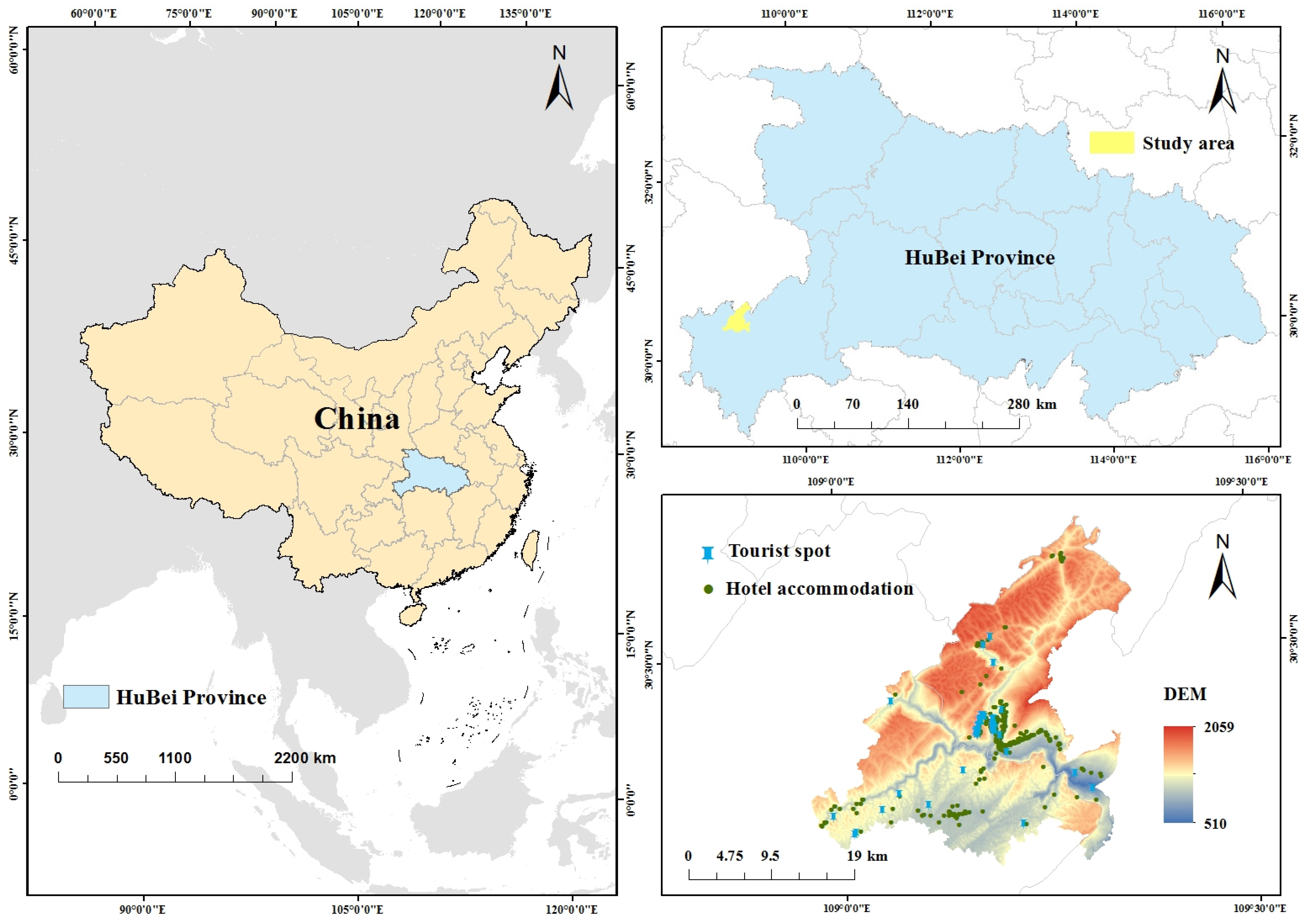
Figure 1. The location of the research area in China and the distribution of tourist attractions and hotel accommodation locations within the geological park in 2020.
Land 14 02262 g001
Figure 2. The geological heritage and distribution of other natural resources of Enshi Grand Canyon—Tonglongdong Cave Geopark (on 27 March 2024, Enshi Grand Canyon—Tonglongdong Cave Geopark was included in the World Geological Park Network List, The pink lines represent the provincial boundaries of Hubei Province).
Land 14 02262 g002
Figure 3. Research framework.
Land 14 02262 g003
Figure 4. The comprehensive ecosystem service index in the study area from 2010 to 2020. Higher index values indicate stronger ecosystem service capacity in the respective region: (a) 2010; (b) 2015; (c) 2020.
Land 14 02262 g004
Figure 5. Contribution characteristics and spatiotemporal changes in influencing factors for ESs: (a) Temporal changes in the contribution rates of various influencing factors for ESs. (b) The contribution percentages (%) of different types of influencing factors in 2010, 2015, and 2020. Note: This figure shows the significant influencing drivers identified by GTWR.
Land 14 02262 g005
Figure 6. The impact of different tourism elements based on BRT on ecosystem services: (ac) The influence on ecosystem services with increasing distance from the road in 2010, 2015, and 2020. (df) The degree of influence on ecosystem services with increasing distance from residential areas in 2010, 2015, and 2020. (gi) The influence on ecosystem services with increasing distance from hotels in 2010, 2015, and 2020. (jl) The influence on ecosystem services with increasing distance from tourist attractions in 2010, 2015, and 2020.
Land 14 02262 g006
Figure 7. The impact of different tourism elements on ecosystem services based on GTWR: (ac) The spatial distribution patterns of the influence of distance from the road on ecosystem services in 2010, 2015, and 2020. (df) The spatial distribution patterns of the influence of distance from residential areas on ecosystem services in 2010, 2015, and 2020. (gi) The spatial distribution patterns of the influence of distance from hotels on ecosystem services in 2010, 2015, and 2020. (jl) The spatial distribution patterns of the influence of distance from tourist attractions on ecosystem services in 2010, 2015, and 2020. Note: This figure shows the significant influencing drivers identified by GTWR.
Land 14 02262 g007
Figure 8. The impact pathways of different influencing factors on ESs. Arrow directions indicate the direction of effects between factors: red arrows denote significant positive relationships, blue arrows denote significant negative relationships, and gray arrows represent non-significant relationships. Numbers adjacent to arrows indicate standardized path coefficients (β). The SEM was constructed to elucidate the pathways of the key driving factors identified as the most influential by the prior Boosted Regression Tree analysis: (a) 2010; (b) 2015; (c) 2020. Note: * indicates p < 0.05, ** indicates p < 0.01, and *** indicates p < 0.001.
Land 14 02262 g008
Table 1. Data and sources.
DataResolution/mData Source
Natural factorsSoil type1000Resource and Environmental Science Data Platform (https://www.resdc.cn/) (accessed on 21 August 2024)
Digital elevation model (DEM)30Geospatial Data Cloud (https://www.gscloud.cn/) (accessed on 12 May 2023)
Normalized difference vegetation index (NDVI)500Resource and Environment Science Data Center(https://www.resdc.cn/) (accessed on 14 August 2024)
Slope1000National Earth System Science Data Center
http://www.geodata.cn (accessed on 18 May 2025)
Aspect1000National Earth System Science Data Center
http://www.geodata.cn (accessed on 18 May 2025)
Temperature1000National Earth System Science Data Center
http://www.geodata.cn (accessed on 18 May 2025)
Precipitation1000National Earth System Science Data Center
http://www.geodata.cn (accessed on 18 May 2025)
Social and economic
factors
Population density1000National Earth System Science Data Center
http://www.geodata.cn (accessed on 27 May 2025)
GDP per capita1000National Earth System Science Data Center
http://www.geodata.cn (accessed on 27 May 2025)
Land use and land cover change (LUCC)30The 30 m annual land cover datasets and its dynamics in China from 1985 to 2023 (https://doi.org/10.5281/zenodo.12779975) (accessed on 12 March 2025)
Tourism factorsDistance from roads\Open street map
(http://www.openstreetmap.org/) (accessed on 19 June 2024)
Distance from tourist spots\Open street map
(http://www.openstreetmap.org/) (accessed on 19 June 2024)
Distance from hotels\Open street map
(http://www.openstreetmap.org/) (accessed on 26 June 2024)
Distance from residential areas\Open street map
(http://www.openstreetmap.org/) (accessed on 26 June 2024)
Table 2. Algorithms of the InVEST model.
Ecosystem
Service
Algorithm
Water Yield Y ( x ) = 1 A E T ( x ) P ( x ) × P ( x )
where Y(x) is the annual water yield (mm) at grid cell x; AET(x) is the annual actual evapotranspiration (mm); and P(x) is the annual precipitation (mm) [32,33,34].
Habitat Quality D x j = r = 1 R   J = 1 Y r   ω r r = 1 R   ω r r y i r x y β x S j r
where Dxj is the habitat degradation index of grid cell x in land cover type j; R is the number of threat factors; Yr is the number of grid cells of threat factor r; wr is the weight of threat factor r; ry is the stress value of grid cell y; irxy is the threat level of threat factor r in grid cell y to grid cell x; βx is the accessibility level of threat factors to grid cell x; Sjr is the sensitivity of land cover type j to threat factor r; Qxj is the habitat quality index of grid cell x in land cover type j; Hj is the habitat suitability index of land cover type j; z is a normalization constant (default value 2.5); and K is the half-saturation parameter (set to 0.5 in this study, typically half of the maximum habitat degradation value). The influence range of threat factors and the sensitivity of habitat types to threat factors were set with reference to [35].
Soil RetentionSD = RKLSUSLE = R × K × LS × (1 – C × P)
In the given formula, SD denotes the total annual soil retention (t·hm−2), RKLS refers to the potential soil erosion (t·hm−2), and USLE indicates the actual soil erosion (t·hm−2). R is the rainfall erosivity factor, K is the soil erodibility factor, and LS is the slope length–steepness factor. C represents the cover management factor, and P is the support practice factor. The parameterization of these factors (e.g., C and P) was conducted as described in Reference [36].
Carbon Storage C = C i a b o v e + C i b e l o w + C i s o i l + C i d e a d
where C is the annual carbon sequestration (t·hm−2); Ci-above is the aboveground biomass carbon density (t·hm−2) for land use type i; Ci-below is the belowground biomass carbon density (t·hm−2); Ci-soil is the soil organic carbon density (t·hm−2); and Ci-dead is the dead organic matter carbon density (t·hm−2). The carbon pool density values for each land cover type refer to [37].
Table 3. The 9-degree classification method.
ScaleSignification
1Indicates that one factor is of the same importance as the other.
3Indicates that one factor is slightly more important compared to the other factor.
5Indicates that one factor is significantly more important than the other when comparing two factors.
7Indicates that one factor is more significant and important compared to the other factor.
9Indicates that one factor is extremely more important than the other when comparing two factors.
2, 4, 6, 8The median of the above two adjacent judgments.
count backwardsThe judgment aij comparing factor i with factor j, then the judgment aij comparing factor j with factor a i j = 1 a i j .
Table 4. Diagnostic results of GTWR and OLS models.
R2RSSAICc
GTWROLSGTWROLSGTWROLS
0.570.434.615.65704.25843.67
Table 5. BRT cross-validation results.
YearTraining Set Pearson Correlation CoefficientTest Set Pearson
Correlation Coefficient
R2RMSE
20100.860.750.740.029
20150.860.770.730.028
20200.880.750.770.028
Disclaimer/Publisher’s Note: The statements, opinions and data contained in all publications are solely those of the individual author(s) and contributor(s) and not of MDPI and/or the editor(s). MDPI and/or the editor(s) disclaim responsibility for any injury to people or property resulting from any ideas, methods, instructions or products referred to in the content.