30 Years of Land Cover Change in Connecticut, USA: A Case Study of Long-Term Research, Dissemination of Results, and Their Use in Land Use Planning and Natural Resource Conservation

Abstract

Remotely sensed land cover data can be a tremendous resource to land use decision makers, yet there is often a disconnect between the worlds of remote sensing and local government. The Connecticut’s Changing Landscape project is focused on bridging this gap. The project analyzes changes to the state’s landscape using Landsat-derived 30-m land cover and cross-correlation analysis. It includes seven dates spanning 30 years, from 1985 to 2015. During this period an additional 4.7 percent of the state was converted to development-related land covers, with corresponding losses to forest and agricultural land. New development was for the most part in attenuated patterns rather than concentrated near existing developed areas. Additional land cover analyses were conducted of agricultural areas, riparian corridors, core forest, and watershed imperviousness, to more closely examine issues of sustainability. Particular care is taken to make research findings accessible, understandable, and usable for the public through traditional outreach methods, and increasingly through internet mapping technology. As a result, the project has become a widely used resource informing the work of state, regional and local governments, nonprofit organizations, and researchers. A more concerted effort to integrate research and outreach is needed to ensure that land cover research has an impact on issues of land use and sustainability.

1. Introduction

Land use is an issue that cuts across many scientific disciplines and societal considerations. Among these are human health [1,2], climate change and adaptation [3,4], and the conservation and management of a long list of natural resources, including water, forest, and wildlife habitat [5,6]. The science of remote sensing has brought tremendous analytical power to the study of land cover, in which pixels from imagery have been classified to discrete and quantifiable land cover categories. However, in many cases there remains a disconnect between the global or national scale of land cover data and the more local setting of land use decision making.

Land cover data are now widely available in the United States. The Landsat-based 30-m resolution National Land Cover Database, produced by a consortium of federal agencies, covers the entire region of the “lower 48” states. The most recent release of the dataset (in 2019) has seven years of land cover for the years 2001, 2003, 2006, 2008, 2011, 2013, and 2016 [7,8]. These data are being widely used for a host of analytical purposes, but not necessarily for direct support of land use planning. This is likely due to several reasons. First, these data are largely the purview of federal and state agencies, and in much of the United States land use decision making occurs primarily not at the federal or state level but at the county and local (municipal) level [9]. In the New England region of the USA, land use is almost exclusively the province of municipal government. For instance, Connecticut, the third smallest state in the country at 12,887 square kilometers (km²), has 169 municipal political entities, each with its own land use plan and regulations. Second, as with much research there remains a frequent disconnect between the generation of information via that research and the integration and use of the subsequent information by decision makers [10,11]. Third and last, land cover information derived from moderate resolution (30-m) imagery, while still an industry standard, is often assumed to be too coarse for uses related to land use planning at the local level. Land use information used during the land use decision making process—for instance, development plans or zoning maps depicting existing and permitted land uses, is typically oriented toward the individual parcel (property) level, often incorporating detailed planimetric data such as building footprints and street edges. Moreover, in recent years, high resolution imagery available at the touch of a finger on phones and other mobile devices has served to raise expectations with regard to the granularity of remotely sensed data.

Given all this, can 30-m land cover data make a substantive contribution to sustainable land use planning in regions where land use decision making is local? This paper describes a long-term, ongoing effort in Connecticut, USA, which demonstrates that land cover data derived from 30-m imagery have had a wide array of impact on local land use issues.

The project is the result of the coming together of two separate entities at the University of Connecticut (UConn), the Laboratory for Earth Resources Information Systems (LERIS), in the Department of Natural Resources and the Environment, and the Department of Extension, both within the College of Agriculture, Health, and Natural Resources. Researchers in LERIS began producing Connecticut-specific land cover data in the early 1990’s [12,13]. In 1991, the Long Island Sound Study, a federal–state research and management partnership administered by the U.S. Environmental Protection Agency, used the LERIS 1990 land cover dataset to estimate stormwater-related nitrogen loadings to Long Island Sound. The Sound is a large estuary between Connecticut and New York’s Long Island, close to the New York City area, that experiences the low oxygen condition known as hypoxia due to nutrient pollution [14].

UConn Extension (outreach) faculty with expertise in land use and water quality were involved in the Long Island Sound Study and realized the educational potential of the land cover data above and beyond its use in determining nitrogen loadings. As a result, in 1991 a partnership developed between Extension and LERIS faculty that eventually resulted in a new outreach program called Nonpoint Education for Municipal Officials (NEMO). NEMO used the LERIS land cover data to educate local land use decision makers on the status of their landscape and the relationship of that landscape to the health of their water resources. NEMO became a successful program and continues to this day, at least in part because of its innovative use of geospatial technology and the fact that the land cover data—as opposed to land use data—were something new and informative for local officials, showing them not what was planned or permitted but what was actually the state of their landscape [15,16,17].

Although the land cover data proved to be a powerful education tool, NEMO and LERIS principals recognized that land cover “change” data would be even more so, giving local officials not only a feel for the state of their community but a sense of “how they got there” and, perhaps, where they might be headed under the status quo. This realization gave rise to the Connecticut’s Changing Landscape (CCL) project, which in turn became the basis for the 2002 formal merger of the two entities into the new UConn Center for Land Use Education and Research (CLEAR). CCL is based on the conviction that in order to have an impact on land use decision making, and thus, sustainability, land cover research must be accompanied by a determined effort to make research results both accessible and understandable to multiple audiences. The rest of this paper provides an overview and retrospective of the CCL. Highlights of key research findings are presented, but equal attention is paid to the methods and results of the project dissemination effort.

2. Materials and Methods: Research

2.1. Overall Land Cover Change Analyses

The CCL project uses remote sensing technology to identify and map changes in the state’s major land cover categories over time. CLEAR developed the CCL project specifically to enable “apples-to-apples” comparisons of multi-temporal land cover data sets based on 30-m pixel Landsat imagery [18]. Landsat is the longest continuously operated program for the collection of satellite imagery of the Earth. The first satellite, Landsat 1 (originally named ERTS-1), was launched in 1972, with the most recent satellite, Landsat 8, being launched in 2013. Over the years, technological advances have resulted in changes in sensor design used to collect imagery. Landsat 4 was the first satellite to carry the Thematic Mapper sensor which collected imagery at 30-m spatial resolution over six spectral reflectance bands (blue, green, red, near-infrared, and two short wave infrared). Although there have been modifications and improvement to the sensors over subsequent satellites, the initial 30-m spatial and six band spectral resolutions have remained similar up through Landsat 8 with the Operational Land Imager sensor, providing more than 35 years of comparable image collection.

The land cover datasets of the CCL date back to 1985, the first year for which cloud free imagery of this resolution was available for the Connecticut area. Hurd et al. [18] used cross-correlation analysis—which employs statistical analysis to identify pixels indicating a potential land cover change between images—to produce a consistent set of land cover data that one can assess for land cover change over time [19,20]. To create the 1990 classification, potentially changed pixels from 1985 were identified, classified and then merged with the “no change” pixels of the 1985 classification. This process was repeated for the 1995 and 2002 classifications for the original study, and has subsequently been done for the 2006, 2010, and 2015 classifications, resulting in a seven date, 30-year record of land cover and land cover change within the state. All classification datasets identify the same 12 land cover categories, with an emphasis on identification of change occurring in four major land cover categories of interest: developed land, turf and grass, agricultural field, and forest [18] (

Table 1. Descriptions of four major land cover categories in Connecticut’s Changing Landscape (CCL) study.

Class	Description
Developed (red)	High-density built-up areas typically associated with commercial, industrial, and residential activities and transportation routes. These areas can be expected to contain a significant amount of impervious surfaces: roofs, roads, and other concrete and asphalt surfaces.
Turf and Grass (yellow)	A compound category of undifferentiated maintained grasses associated mostly with developed areas. This class contains cultivated lawns typical of residential neighborhoods, parks, cemeteries, golf courses, turf farms (areas where sod is grown for commercial sale), and other maintained grassy areas. Also, includes some agricultural fields due to similar spectral reflectance properties.
Agricultural Field (brown)	Includes areas that are under agricultural uses such as crop production and/or active pasture. Also, likely to include some abandoned agricultural areas that have not undergone conversion to woody vegetation.
Forest (green)	A combination of multiple land cover classes including deciduous forest, coniferous forest, forested wetland and utility right-of-way (this class is only identified in forested areas).

) (Figure 1).

Summary statistics were generated on the extent of each of these classes for each of the seven dates, and change between dates. As more completely described in the dissemination section, the data were analyzed at the state, municipal, and watershed levels. Change maps were produced that either showed areas of change (Figure 2a) or averaged change data for relevant units such as towns or watersheds (Figure 2b). As the project period has lengthened and the number of datasets has increased, maps and graphics on land cover change have increasingly focused on the entire period rather than the intervening intervals, although data on each of the seven dates is always available. Change is measured in several ways depending on the topic at hand: absolute change (area²⁰¹⁵–area¹⁹⁸⁵); relative change (percent²⁰¹⁵–percent¹⁹⁸⁵⁾); and relative rate of change ([area²⁰¹⁵–area¹⁹⁸⁵]/area¹⁹⁸⁵).

2.2. Land Cover Change in Landscapes of Importance for Sustainability

In addition to basic land cover change maps, CLEAR also has conducted several subsidiary analyses that use the land cover as the basis for a closer examination of landscape characteristics of particular interest when considering issues of sustainability and natural resource protection. The four analyses are (1) land cover over agricultural soils, (2) land cover in riparian areas, (3) forest fragmentation, and (4) watershed impervious cover. Due to funding constraints, not all of these four subsidiary studies have been done for all seven dates. A fifth analysis, looking at urban growth patterns, was developed for the original four-date (1985, 1990, 1995, and 2002) data set [21] but has not since been applied.

At several dates various aspects of the CCL analyses (most often land cover change, riparian change, and impervious cover change) have been conducted for a slightly different geographic area known as the “Lower Long Island Sound Watershed.” These studies were commissioned by the federal/state Long Island Sound Study, and in addition to almost all of Connecticut include areas of Massachusetts, Westchester County, NY, and Long Island, NY, which drain to Long Island Sound. Results of these studies are not reviewed in this paper, although the use of the data by the Long Island Sound Study is included in the Discussion section.

Land cover over agricultural soils: The first of the subsidiary studies analyzed land cover and land cover change over areas designated as having “prime” or “important” agricultural soils, a national dataset produced by the U.S. Department of Agriculture [22]. Through the 1850’s, Connecticut had largely been deforested for agricultural purposes, but since the early 1900’s much of that agricultural land has been converted, first reverting to forest and since the 1950’s, to urban/suburban land covers. Since many of the characteristics of good agricultural land (flat and well-drained) are also conducive to development, we undertook this analysis to see if areas best suited for agriculture were being disproportionately converted to urban/suburban uses.

The first step analyzed the change in the agricultural field class of the land cover for all dates for the entire state. The next analysis incorporated the Farmland Soils interpretation of the Soil Survey Geographic (SSURGO) database [22] for the State of Connecticut, available from the Connecticut Department of Energy and Environmental Protection. This included both prime and important farmland soils. For each date, the land cover occurring on these farmland soils was summarized and compared to the state average.

Riparian Area Analysis: The second analysis looked at land cover and land cover change in streamside, or riparian areas. These corridors can harbor high biodiversity and provide ecological corridors as well as perform such functions as stormwater infiltration and filtration, stormwater management, flood water management, streambank stabilization, and sediment trapping [22,23]. In addition, riparian zones often serve as a sink for nitrogen [24,25,26]. Again, the main purpose was to see how land cover change in these areas varied among towns and watersheds, and compared to overall change at the town and the state levels. Connecticut has enabling legislation creating Inland Wetland and Watercourse Commissions in each town that review development proposals in riparian and wetland areas for environmental impacts [27]; we wanted to see if the land cover data could shed light on what effect this legislation was having. Although the most common review zone used by Connecticut towns is 100 feet (30 m) to either side of a stream or waterbody, we felt that, at approximately one 30 m pixel in width, this was too narrow a zone for reliable results. In addition, some of the natural resource functions of riparian areas, particularly those related to providing wildlife corridors, are thought to require widths in excess of 30 m [28,29,30]. For these two reasons, we used a riparian corridor analysis width of 300 feet (about 91 m).

First, we created a seamless, statewide, continuous GIS layer of water edges that included not only stream lines (as determined from statewide hydrography data) but also shorelines of rivers, wetlands, tidal marshes, and waterbodies that intersected the stream lines [31] (Figure 3a, blue line). The land determined to be part of the riparian corridor was 300 feet (91 m) from the continuous line (minus the inside of lakes, tidal wetlands, and large rivers) (Figure 3a,b, black line). Land cover existing inside the 300 foot (91 m) corridor was analyzed for land cover category area and for land cover change. Figure 3 shows the process and a sample result from the analysis.

Forest Fragmentation: A landscape fragmentation analysis following a methodology developed jointly by researchers at the European Commission Land Management and Natural Hazards Unit and the U.S. Department of Agriculture (USDA) Forest Service [32,33,34] was adapted by CLEAR researchers and applied to the Connecticut land cover [35,36,37]. Although the percentage of forested land in the state remains high (62–59% over the course of the study), tree cover alone is not a complete indicator of the functional health of forested ecosystems, which can be impacted by proximity to non-forested areas [38]. The forest fragmentation model was developed to allow researchers, land use officials, natural resource professionals, and the public to obtain a better understanding of the health and status of our state’s forested areas.

The maps represent four conditions of forest—core, perforated, edge, and patch—based on a specific input edge width parameter. Input land cover classes are assigned to be either (1) forest, (2) fragmenting (such as development, turf and grass, etc.), or (3) neither, such as water (Figure 4). The edge width indicates the distance within which fragmenting land covers can degrade the forest, and the edge width assigned in fragmentation analysis is dependent on the purpose of the analysis. Based on the literature [39], we used an edge width of 91 m which is approximate to the often used 100 m edge width for general fragmentation studies. In addition to the four forest categories (patch, edge, perforated, and core), the core forest class was further separated into small (less than 250 hectares), medium and large (greater than 500 hectares) based on the size of the contiguous core forest block. These three core forest categories relate to the functionality of the core forests, with large core forests providing improved benefits over small core forests. Change was determined both between study dates and between categories.

Watershed Impervious Cover: The fourth analysis looked at impervious cover, demonstrated to be a reliable indicator of the impact of development on water resources [40,41,42]. This was done by watershed, using the Impervious Surface Analysis Tool (ISAT) developed by CLEAR and the U.S. National Oceanic and Atmospheric Administration (NOAA) in 2000 [43,44]. Impervious surface coefficients were developed for each land cover category by using high-accuracy planimetric GIS data for multiple towns with a range of development density. Impervious surfaces included roads, driveways, sidewalks, parking lots, and building footprints, which were all present in the planimetric data. The planimetric layers were then overlaid with the 12-class land cover to determine, on average, how much of each land cover category area was comprised of impervious surfaces These coefficients were then applied to the entire land cover dataset [43,44].

As noted, there is a robust body of literature on the impact of impervious cover on water resources and the logic follows that watersheds are the most meaningful geographic unit to use in measuring this particular land cover. The ISAT analysis was originally conducted at the USGS 12-digit Hydrologic Unit Code (“HUC-12”) level of watershed, which in our study area average about 77 km² (the national average is about 100 km²) (Figure 5). However, the literature also suggests that the relationship known as the Impervious Cover Model [38], where increasing amounts of impervious cover result in decreasing water quality, is best applied at the small (less than 50 km²) watershed level. For this reason, and because smaller watersheds are more relatable to local land use decision makers, we also have estimated impervious cover for the more than 7000 basins that comprise the smallest level of watershed organization available in Connecticut, which average about 2 km² in size.

2.3. Materials and Methods: Information Dissemination

The land cover research effort has been accompanied by an extensive effort to make the results accessible and understandable for a wide range of users. At the advent of the CCL project in 2004, this was a departure from our previous treatment of research information; although, the NEMO Program was built around the educational power of the land cover data, the data and maps were used within the context of educational presentations to various audiences and were not published on the internet for general consumption. This was partly due to the fact that in the 1990’s and early 2000’s the presentation of maps online was in its very early stages. In addition, there were concerns by the researchers that lay audiences would—either unintentionally or intentionally—misinterpret or misuse the results. In any case, by 2004 the fusion of GIS and internet technology had evolved to the point where there were new ways to convey the data. Given this, the team decided that as long as the derivation and limitations of the data were carefully explained, the benefits of publishing land cover information on the web outweighed any potential abuses [45].

Thus, in January 2004 the first version of CCL, covering the 1985, 1990, 1995, and 2002 study dates, was made public on the CLEAR website. Since the website was targeting non-technical as well as scientific and academic audiences, the maps and data were accompanied by an extensive “About” section that included: metadata; detailed descriptions of the land cover classes; a detailed and illustrated “Viewer Help” page to walk visitors through the use of the online maps; a FAQ (Frequently Asked Questions) section with answers to 15–20 questions such as, “What is the difference between land cover and land use?” and “Why can’t I see my house on your maps?”; and an illustrated “Caution” section that explained the limitations of the data in terms of issues like resolution and mixed pixels. (This section remains a part of the website to this day). The release was accompanied by a front page article in the Hartford Courant, the largest newspaper in Connecticut, entitled “Satellite Pinpoints State’s Sprawl” [46]. Two months later, CCL was the focus of an opinion piece by the researchers in the Courant [47], followed by an editorial the following day that praised the usefulness of the online maps as a state planning tool [48].

The project website was designed to make the research results accessible to a wide range of audiences of varying degrees of geospatial expertise. Data were conveyed in various formats, from static pie and bar graphs to data tables to GIS files available to download, and, of course, maps (from PDFs to an ArcIMS interactive map viewer). Depending on the dataset, the maps were presented as statewide, by town, or by watershed (Figure 6).

In addition to statewide results, land cover and land cover change information was made available in tabular form where the area and percent of each land cover class were reported, along with maps (pdfs and gifs) for each of the state’s 169 municipalities, which is the political level of organization at which most land use decisions are made in Connecticut. The “Your Town” section of the original website allowed the user to select a town and flip through the following: land cover maps of 1985, 1990, 1995, and 2002; a map of land cover change showing what areas had been converted to the “developed” and “turf and grass” classes (the “development footprint”); a map of land cover change showing what land cover these newly developed areas had been before conversion; and a table displaying the data for all dates and all classes, by area and by percentage of town (Figure 7). In addition to the Your Town section there was an identically constructed Your Watershed section, displaying data and maps for drainage basins at the regional (average size 77 km²) and sub-regional (average sized 36 km²) levels mapped by the state. This was in recognition of the fact that for many organizations interested in the ecological impacts of land cover change, the watershed was a more meaningful framework than political boundaries.

Internet mapping technologies are constantly changing and as the project continued, new technologies were implemented. The Your Town and Your Watershed sections were widely used, but required generating a large number of maps (7 maps for each of 169 towns), which had to be pre-created and stored. Although this could be somewhat automated through the use of the Esri DS Mapbook script (now called Data Driven Pages), there was no ability to zoom, explore, or search for a location. By the time the 2010 data were processed, technology allowed for more sophisticated interactive maps due to the development of ArcIMS and then ArcGIS Server and ArcGIS Online. Accordingly, a new website was published with interactive maps comparing 1985 and 2010 data for land cover, riparian cover, and impervious cover data.

At present, the Center has moved to a combination of technologies, again with the ultimate goal of relating project information to as wide an array of user types as possible (Figure 8a). For the 2015 update, CCL information is currently online in five different formats (Appendix A). For the more technically-minded users, the data can be accessed as map services, or for download [49]. The information is also contained in an interactive map viewer which displays the map services interactively with ArcGIS Online and then published using the Esri Web App Builder. The viewer contains land cover maps from all seven dates, change data for the 30-year project period (1985–2015), and status and change data by town for the four major land cover classes—developed land, agricultural fields, forest, and turf and grass (Figure 8b). Interactivity is enhanced by tools such as the “swipe” tool that can facilitate comparison between two map layers.

In addition, there is a “Numbers and Charts” page containing a series of interactive visualizations made using Tableau©, a data visualization software. The data formatting required for this type of (generally business-oriented) software is very different than standard GIS attribute tables, presenting some challenges to “translating” our geospatial data into a form that could be used. However, the results afforded the CCL viewer yet another option to accessing the data. The visualizations highlight the same town or watershed summary statistics that are in the map pop-ups, but Tableau presents the data in the form of charts and tables; thereby, providing a different and useful way to further explore land cover status and change for towns or watersheds. Currently, there are visualization tools for 2015 land cover (Figure 9), 1985–2015 overall change, and incremental change using all seven dates.

Lastly, the information is packaged as a “Story Map.” Story maps use one of a variety of templates created by GIS industry leader ESRI [50]. Here, the Map Journal template was used that enables the combination of interactive maps with other information such as text, videos, and photos (Figure 10). The Map Journal Story Map is an ideal way to make complex maps and information available to the user because it can be visually appealing, easy to understand, information rich, and serve to guide the user while allowing for exploration in an interesting, multimedia experience. The Connecticut’s Changing Landscape Story Map (Appendix A), using a customized Map Journal template, has been very popular (more in Results section). We expect the continuing evolution of ever more interactive internet mapping technologies to expand further the range of methods for disseminating land cover information in ways that will support decision making.

It is important to note that throughout the life of the project the online presence of CCL has always been “backed up” by CLEAR outreach faculty with workshops, webinars, conference presentations, and other face-to-face dissemination vehicles. We estimate that well over 100 presentations focused on CCL have been made to municipalities, regional councils of government, state agencies, non-governmental organizations, and college classes. In addition, CLEAR is an engagement-oriented center that develops and runs many outreach programs on topics such as water resource protection, land conservation, and climate change adaptation; CCL land cover information is almost always included as part of these programs. This continues the tradition begun in the early 1990’s with the NEMO program and the use of the first Connecticut-specific land cover data set from 1990.

3. Results: Research

Connecticut’s Changing Landscape is a multi-faceted project spanning many years. Since the intent of this paper is to give an overall description of the entire effort, we focus in this section on two or three findings of statewide significance uncovered by each of our analyses.

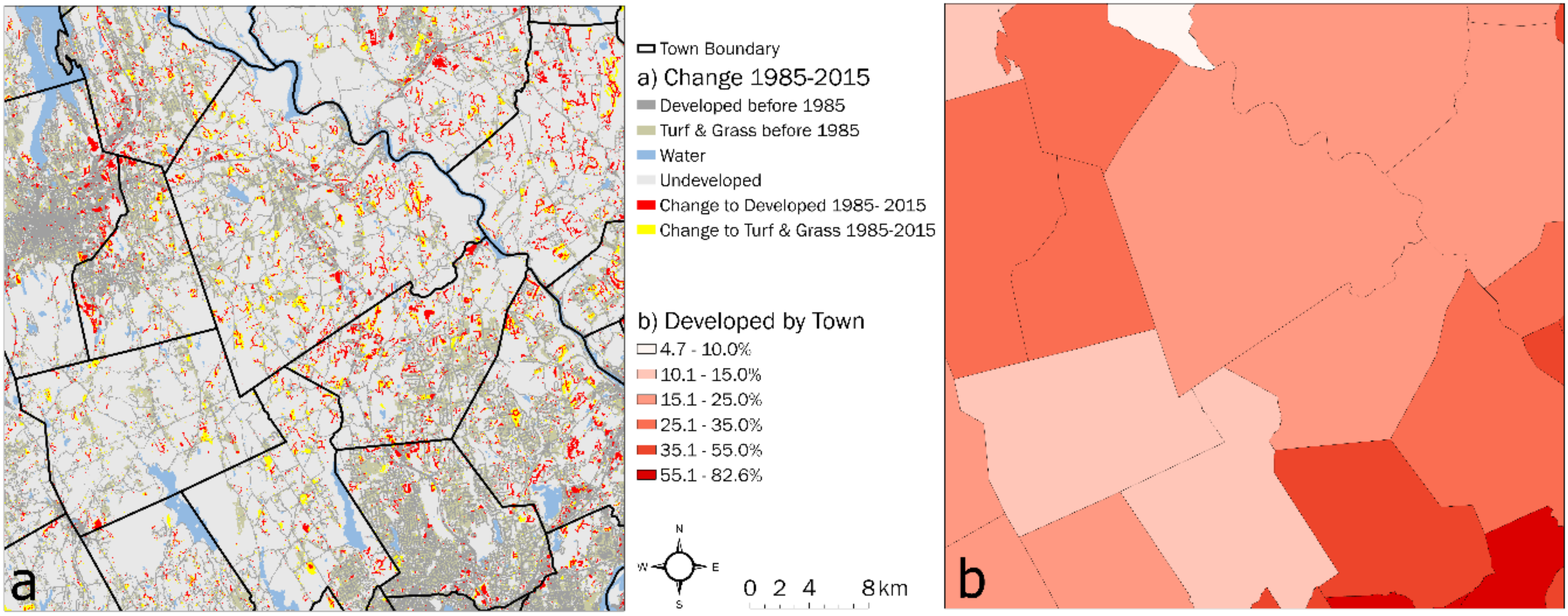
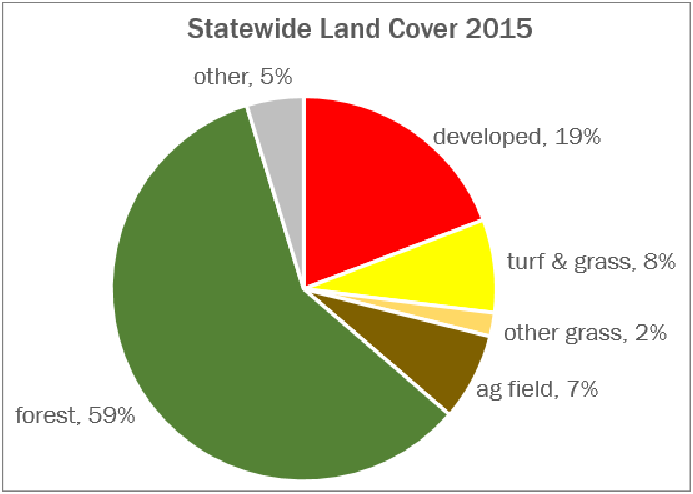
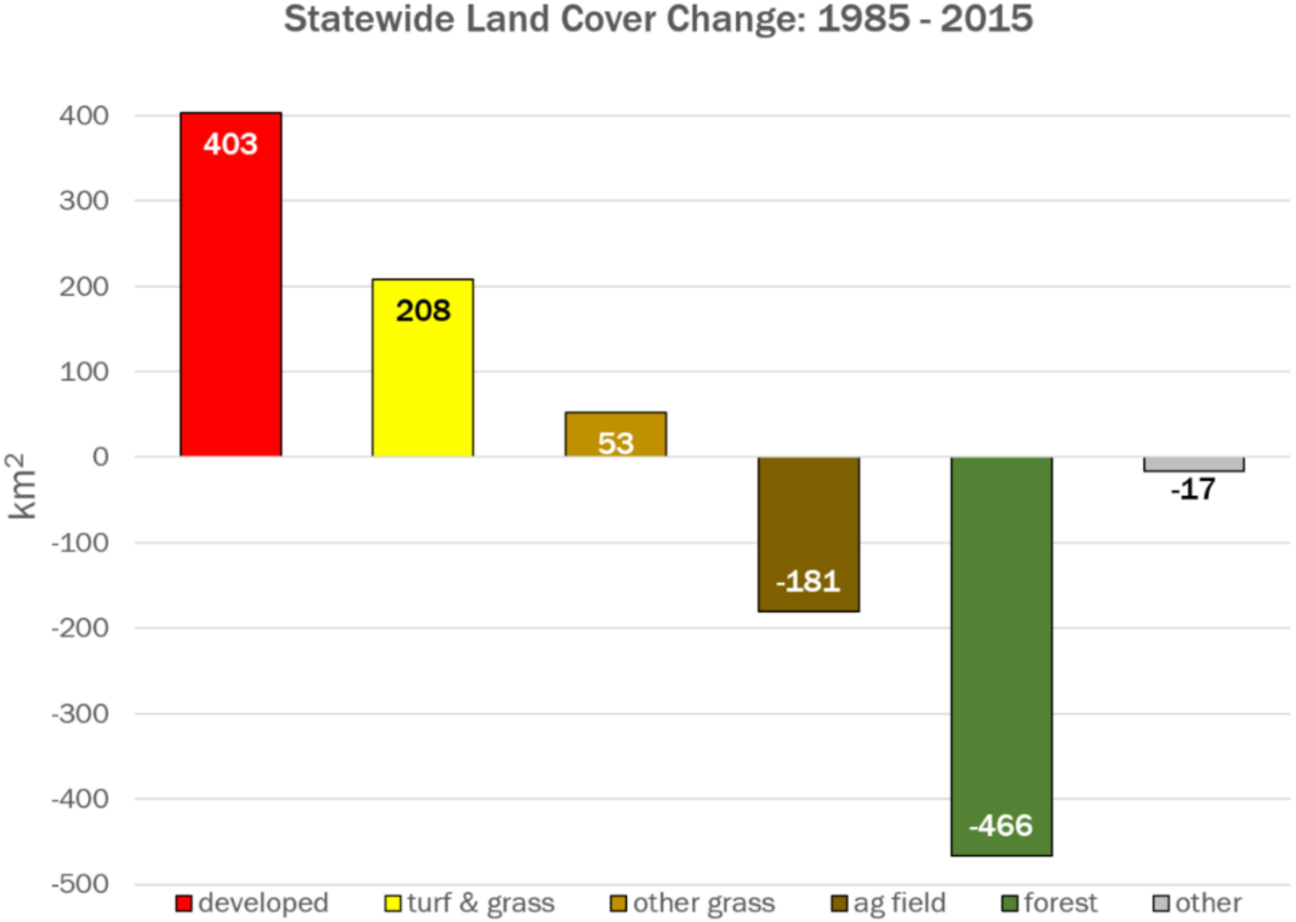
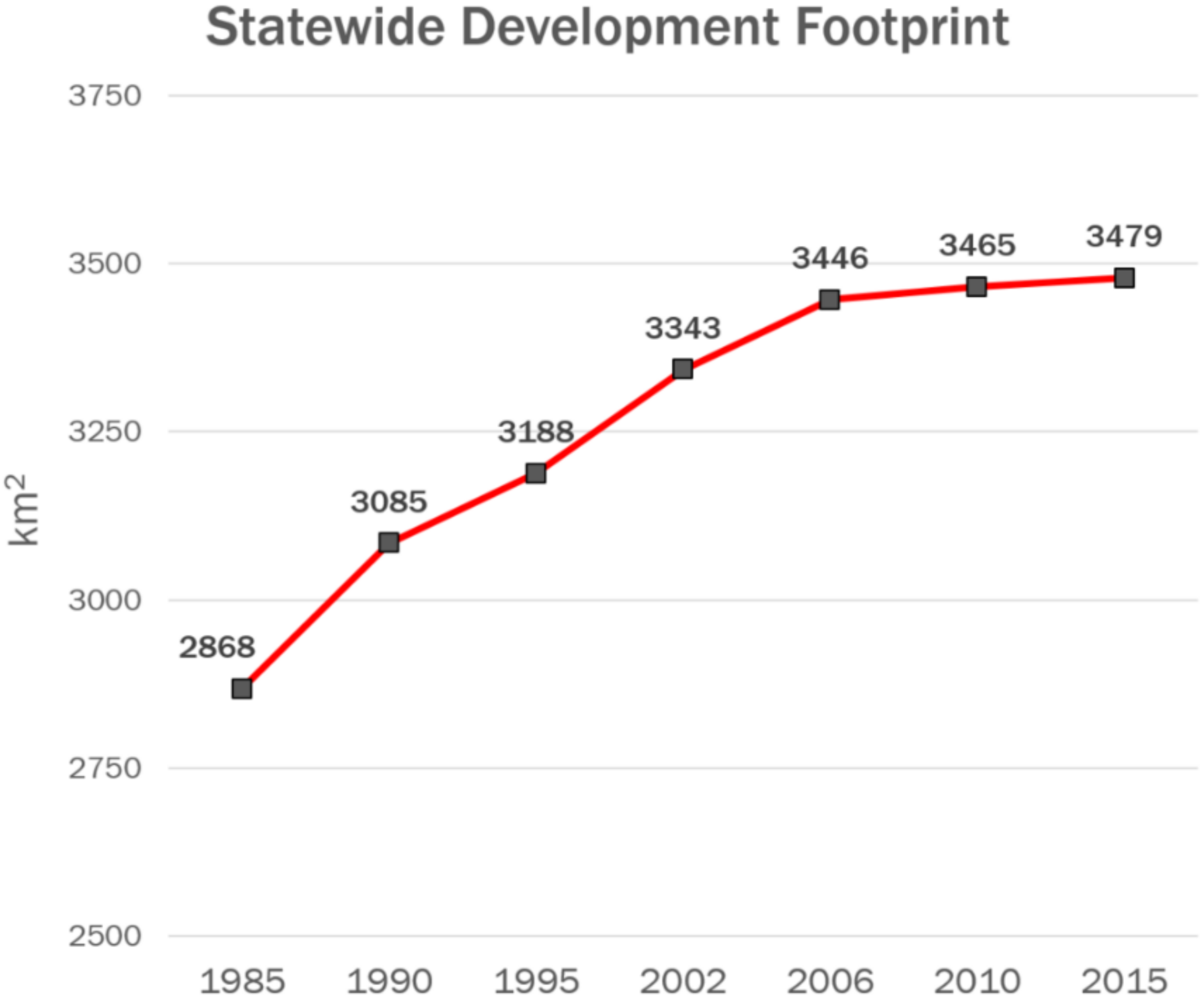
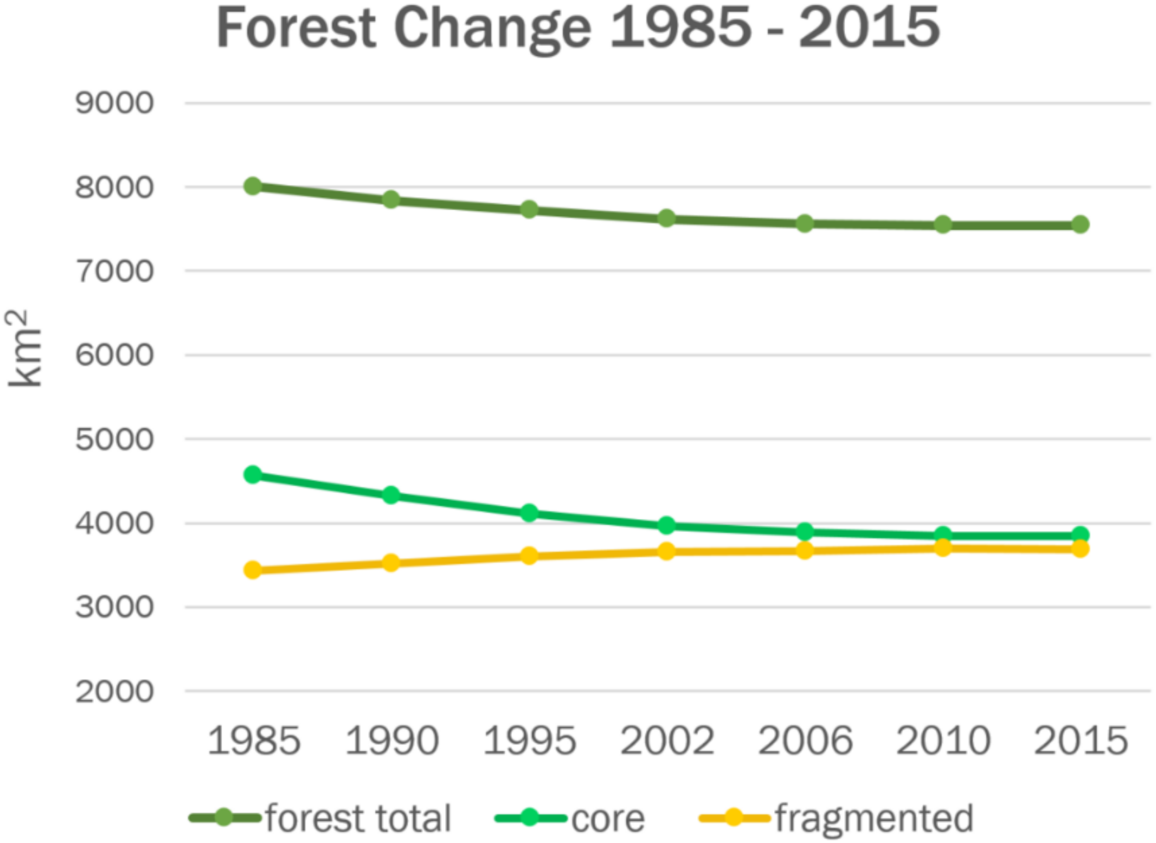
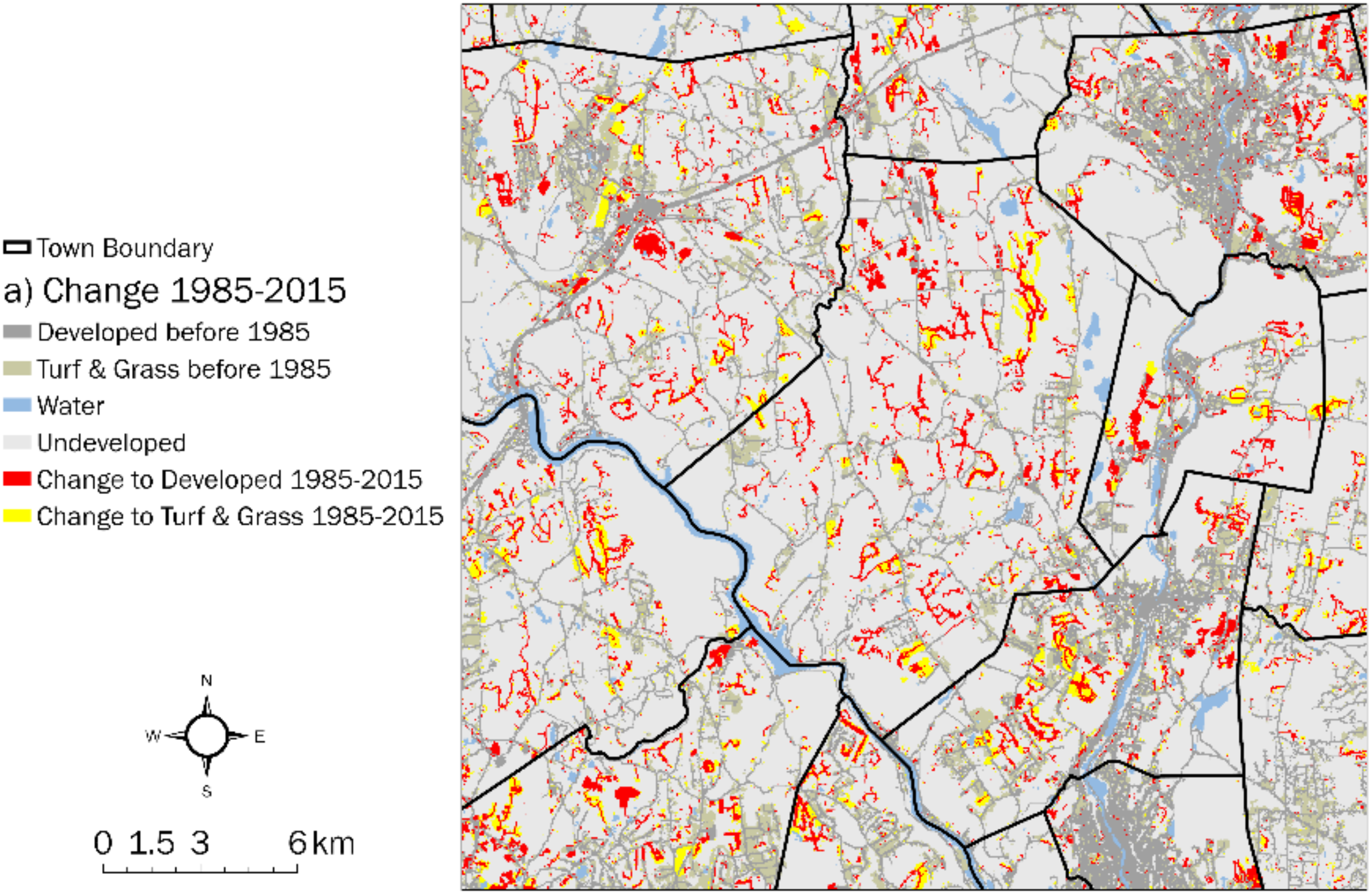
3.1. Statewide Land Cover and Land Cover Change

Forest (a combination of the deciduous forest, coniferous forest, and forested wetland classes) is still by far the largest land cover class in Connecticut, covering about 58.5% of the state in 2015, followed by developed land (19.2%), turf and grass (7.8%), and agricultural fields (7.3%) (Figure 11).

Despite the high amount of forest cover, the change data indicate an urbanizing state, where forest and farmland are being replaced by development. During the 30-year period from 1985 to 2015 Connecticut lost 466 km² of forest cover and 181 km² of agricultural field. These losses were largely balanced by gains in the developed class (403 km²) and the closely associated turf and grass class (208 km²), representing the lawns, golf courses, athletic fields, and parks that are part of the developed landscape (Figure 12). Because the turf and grass category largely represents elements of the landscape that are integrated with the developed category, and because changes in the two categories are closely correlated, we often group them together under the name “urban footprint.” During the 30-year period, these two land covers experienced by far the greatest relative increase over 1985 levels, among the four major land cover categories. Overall, about 4.7% of the state was converted during the 30-year period from other land covers to the urban footprint (about 5.6 hectares per day) bringing the 2015 level to about 27.0% of the state.

Figure 13 shows the growth of the urban footprint during the course of the study. The steepest part of the curve is during the first five-year interval of 1985–1990. This is consistent with economic data that show a strong local economy during the 1980’s, with Connecticut averages for both per capita personal income and per capita Gross Domestic Product (GDP) being above the national average [51]. The flattening of the curve after the 2006 dataset closely tracks the “Great Recession” economic downturn in the U.S., which in Connecticut technically lasted from 2008–2010 but from which the state is still recovering [51].

As noted in the Dissemination Methods section, CCL data are also analyzed at the town (municipal) level, in recognition of the fact that this is the areal unit where most land use decision making takes place. Looking at the growth of development by town in terms of relative percent change ((area²⁰¹⁵–area¹⁹⁸⁵)/area¹⁹⁸⁵) serves to highlight the areas of most rapid growth, which are concentrated not in the traditional transportation corridors as shown by the overall level of development (Figure 14a), but in adjacent areas (Figure 14b). We can roughly define these areas as southeastern Connecticut (Figure 14b,c, yellow circle) (where the construction of two very large casinos has spurred growth), southwest non-coastal Connecticut (Figure 14b,c, yellow dotted circle), and the north-central Connecticut River valley area north of Hartford (Figure 14b,d, red square) (Connecticut’s capital city). Connecticut is situated between the large urban centers of Boston to the northeast and New York to the southwest, and these latter two growth areas are most likely indicative of the expansion of the range of commutation (by car and rail) to these cities. Comparing the map of increased development (Figure 14b) to existing forestland (Figure 14c) shows that much of the new development is in forested areas. Comparing the map of increased development (Figure 14b) to existing agricultural land (Figure 14d) shows an overlap between the northern urbanizing “hot spot” and the most concentrated area of remaining agriculture. This area has long been an agricultural region due to the rich soils of the Connecticut River floodplain.

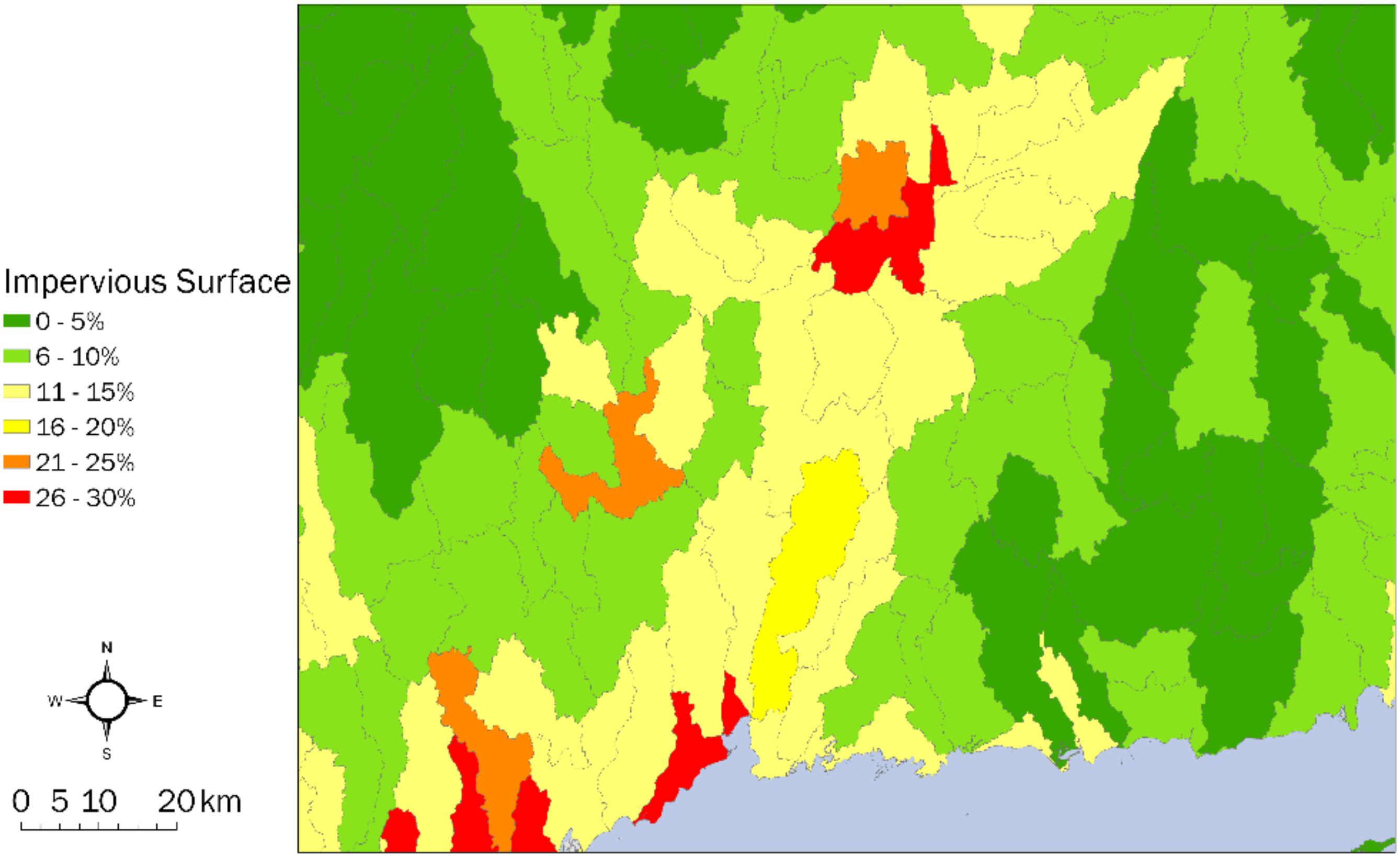
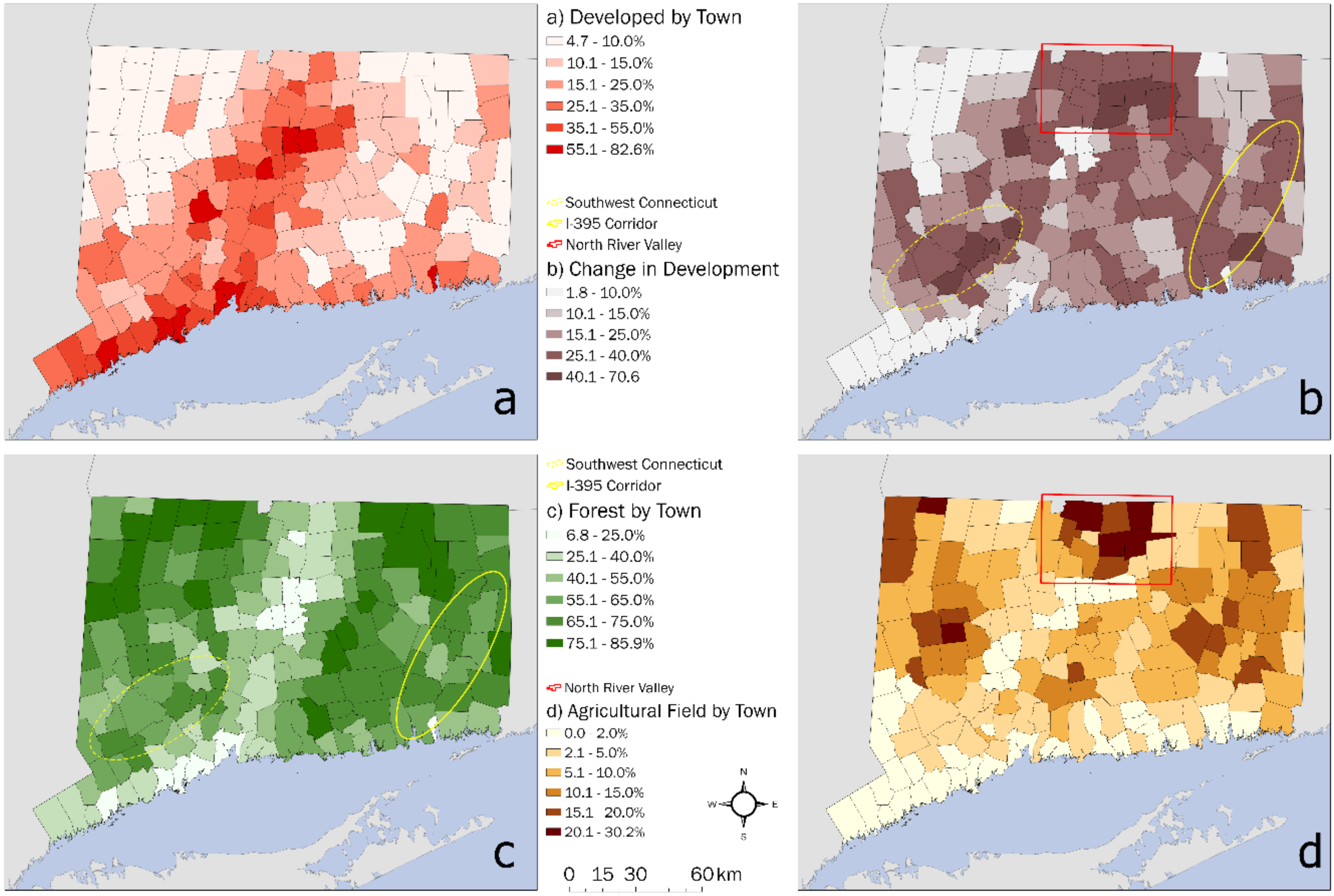
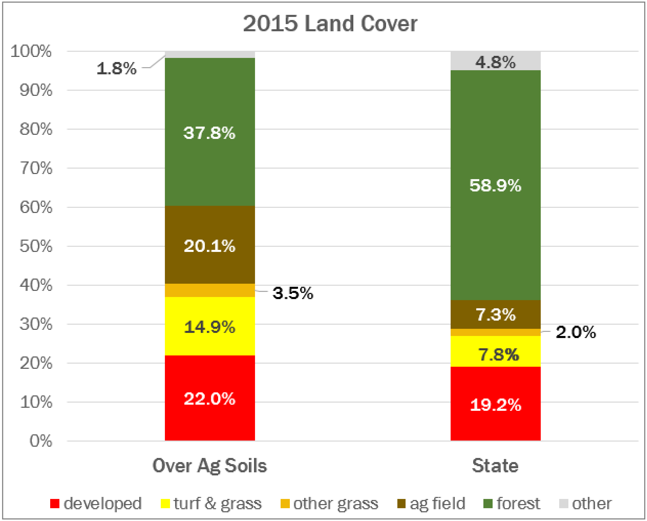
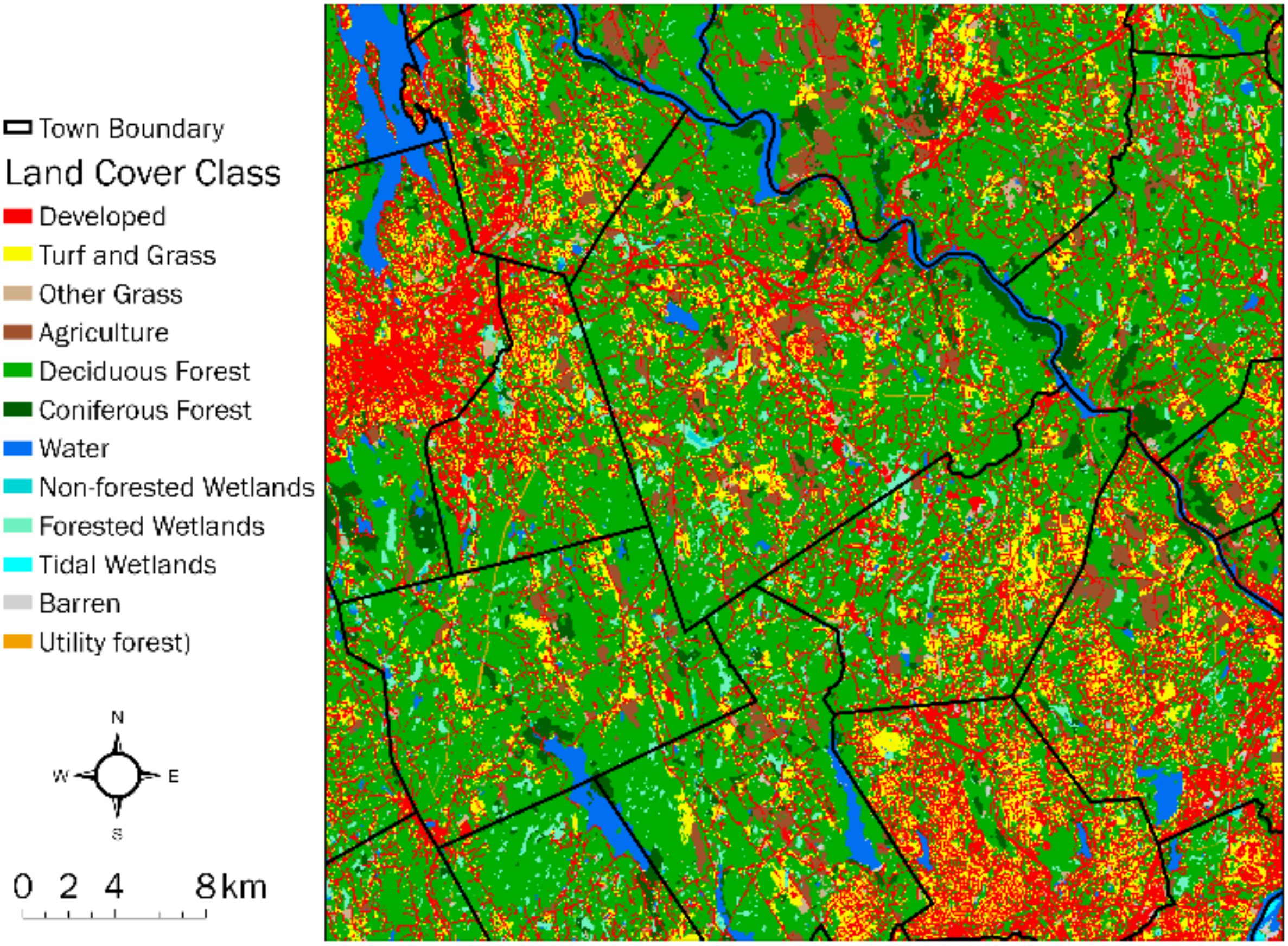
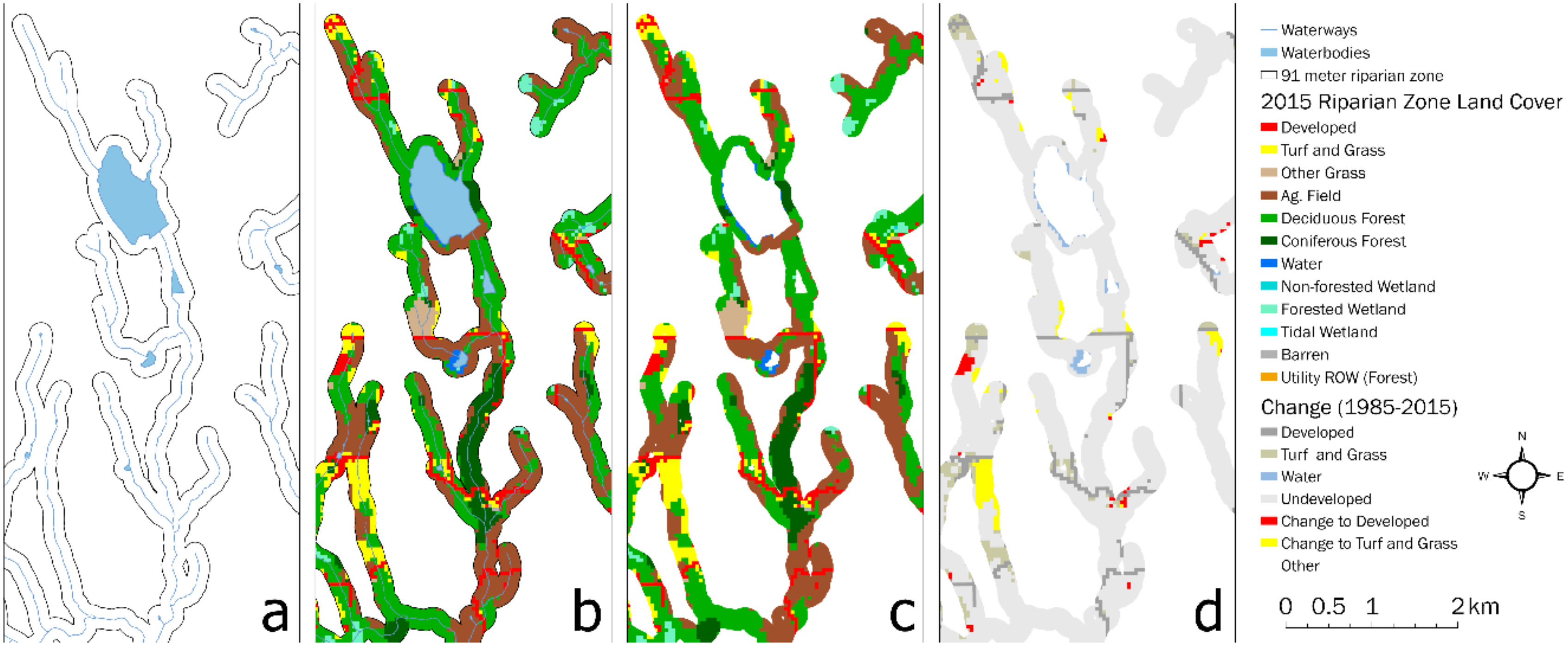
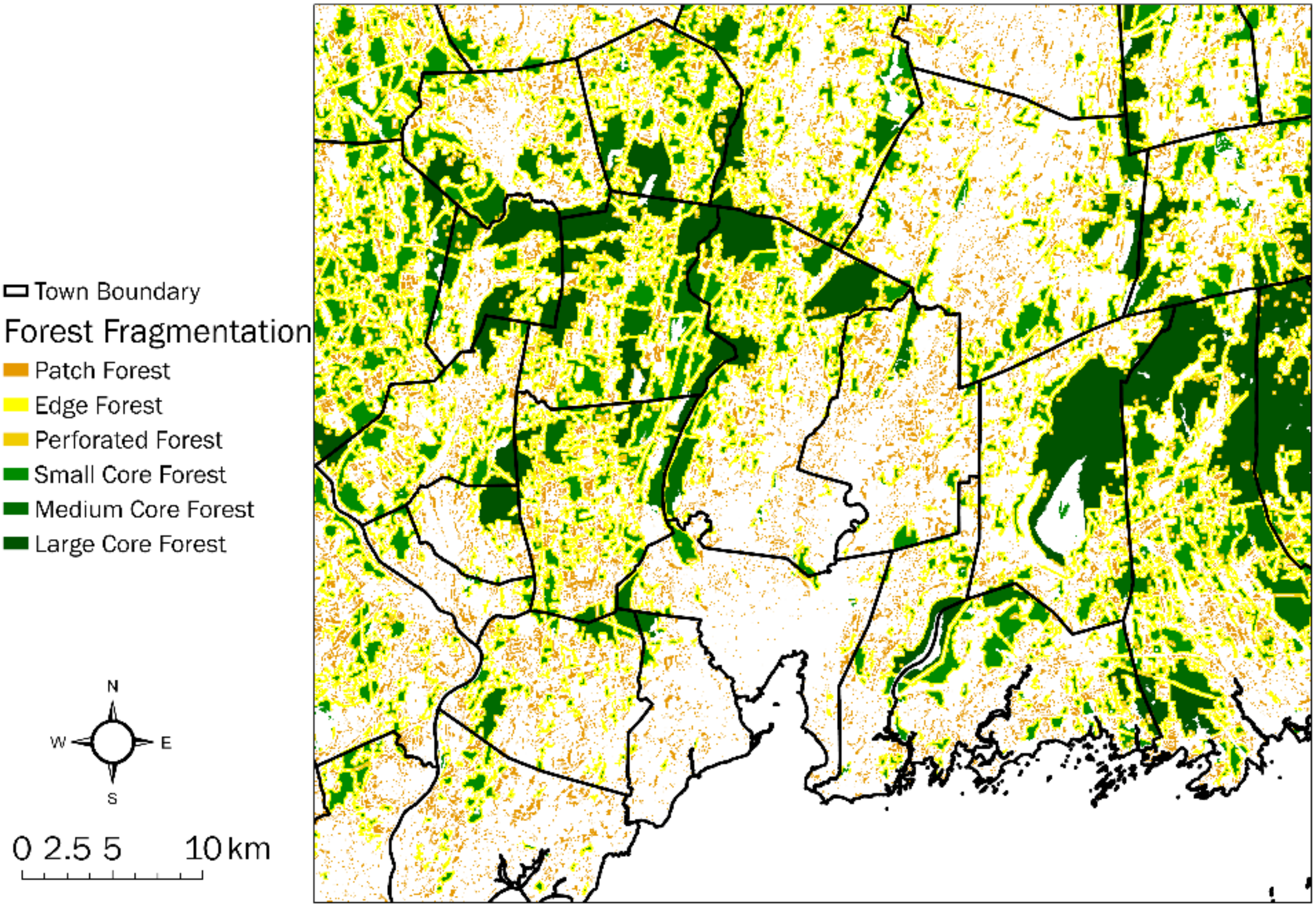
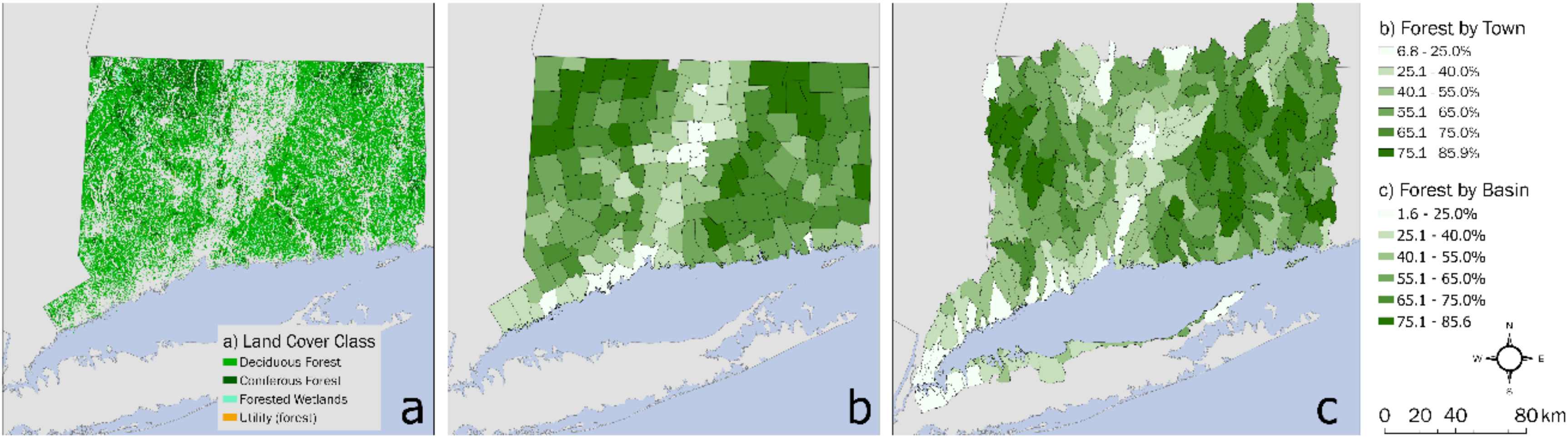
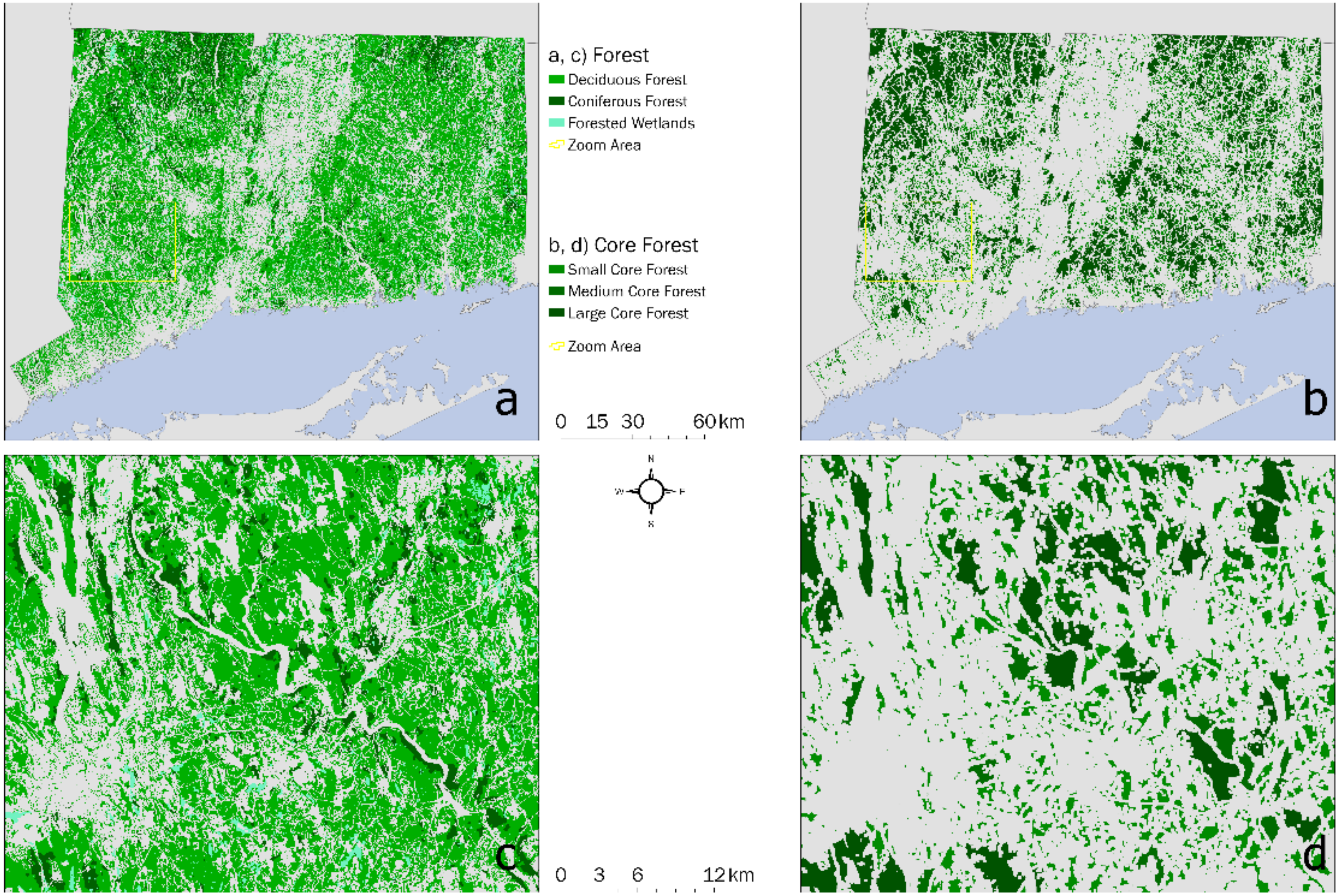
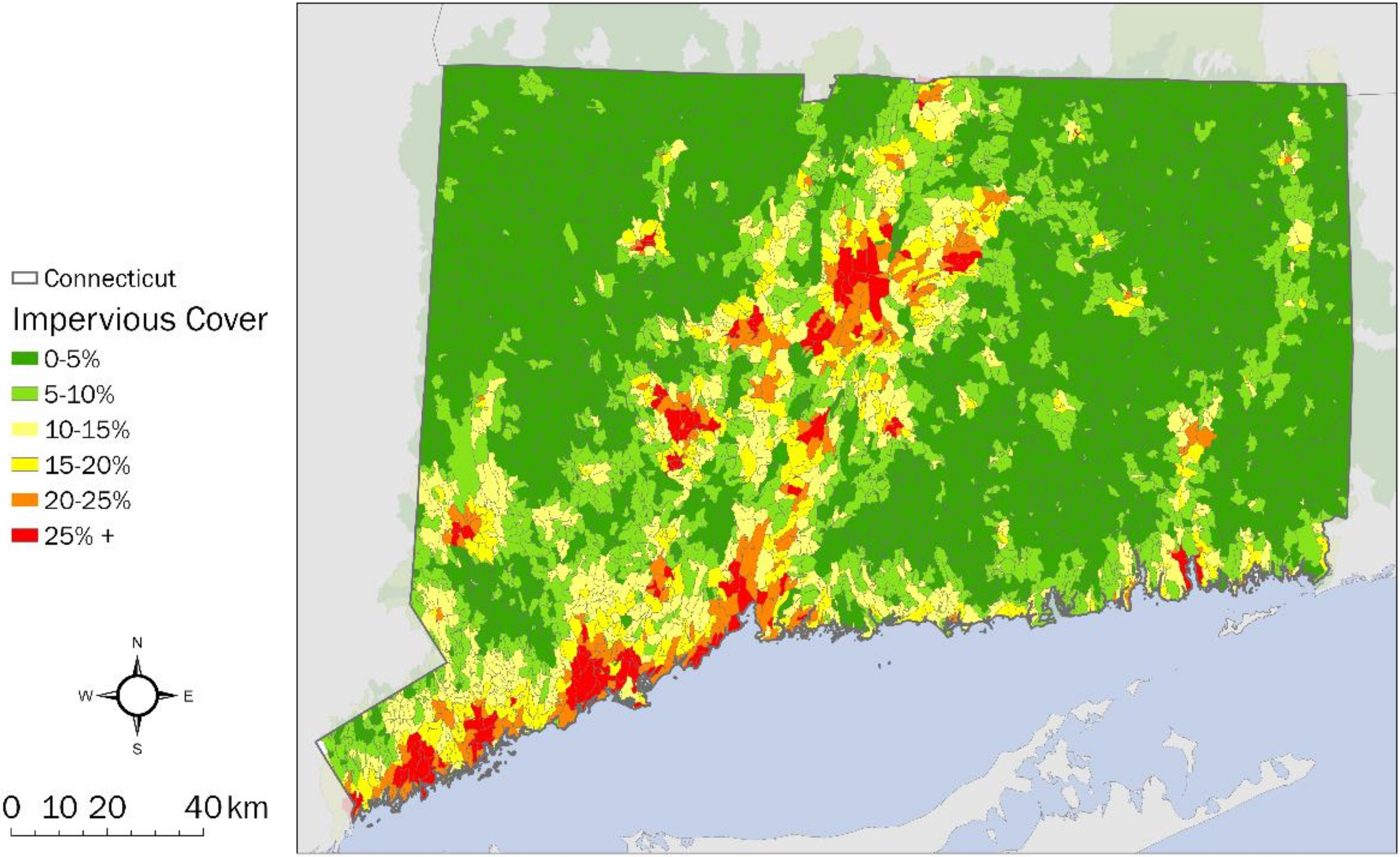
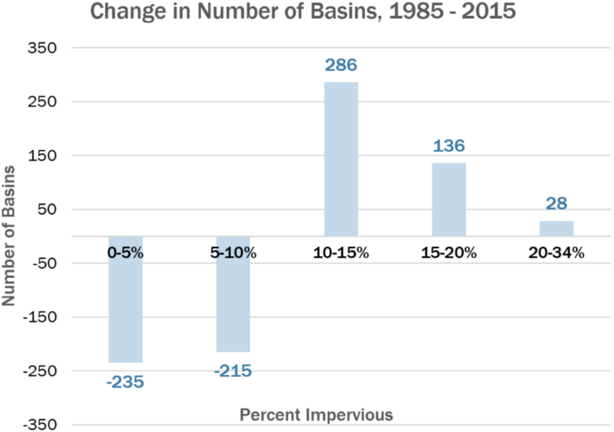
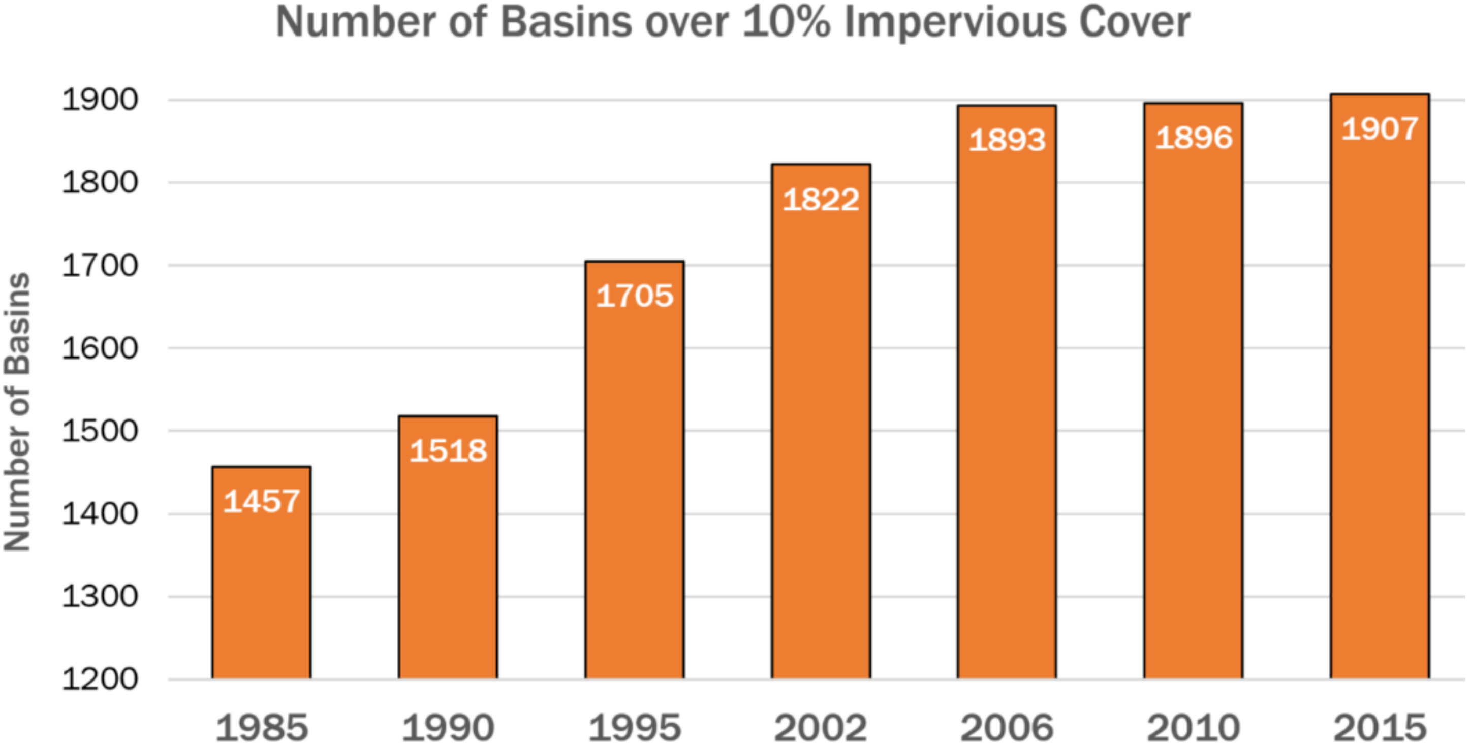
3.2. Land Cover and Land Cover Change in Areas of Special Concern

Important agricultural areas: Agricultural fields accounted for 20.1% of the land cover over prime and important agricultural soils in 2015, down from 24.0% in 1985. Looking at the 2015 data, there are distinct differences between the land cover distribution statewide and that over areas with prime and important agricultural soils as designated and mapped by USDA (Figure 15). In 2015, as might be expected, there is a higher percentage of agricultural fields (20.1%) over agricultural soils than statewide (7.3%). There is also a slightly higher percentage of developed land (22.0% vs. 19.2%) and almost twice the relative amount of turf and grass (14.9% vs. 7.8%). This is likely due to the fact that good agricultural soil areas generally have slope and drainage characteristics conducive to development. Finally, although there is much less forested land over good agricultural soils than statewide (37.8% vs. 58.9%), it is still the largest land cover in these areas by far, reflecting the overall reforestation of the state following the agricultural dominance of the 18th and 19th centuries.

Riparian areas: Land cover composition and land cover change in the 91-m riparian area differed from statewide averages, but only modestly. The amount of forest cover in the riparian area was 63.9%, as opposed to the statewide forest cover of 58.5%. Correspondingly, the amount of the development footprint (developed plus turf and grass categories) was 23.3% in the riparian zone and 27.0% statewide, respectively. During the 30-year period the riparian zone added about 126 km² of development and turf and grass (development footprint). The relative rate of increase of the development footprint ((area²⁰¹⁵–area¹⁹⁸⁵)/area¹⁹⁸⁵ × 100) was only slightly less in the riparian zone than statewide: 18.9% versus 21.6% (

Table 2. Development footprint in riparian corridors versus statewide.

	Area 1985 (Percent)	Area 2015 (Percent)	Change in Percent 1985–2015	Relative Rate of Change
91 m corridor	19.6	23.3	3.7	18.9%
statewide	22.2	27.0	4.8	21.6%

).

The question as to the cause(s) of these differences is not completely answered. Since 1972 the Connecticut General Statutes has required each of the state’s 169 municipalities to establish a local commission empowered to establish “Upland Review Areas,” within which they may regulate activities based on their potential impact to wetlands and watercourses [27]. The width of these areas varies from town to town; the Connecticut Department of Energy and Environmental Protection states that “most towns have delineated the Upland Review Area to be 100 feet, but distances vary across Connecticut from zero to a few hundred feet” [52] (p. 9). These are not “no development” zones but only trigger a review by the local agency, leaving a lot of room for interpretation of a given project’s environmental impacts. Thus, both the width of the review zone and the extent to which local commissions exert their regulatory power vary considerable among towns.

In addition to the wetlands and watercourse review zones, there are additional impediments to development in these areas having to do with the land’s physical suitability for building, particularly the presence of wet soils and steep slopes; both of these conditions can trigger zoning regulations that could restrict or disallow development. In a previous study [31], we looked at these two factors within the 91 m riparian zone using USDA soils data, and found that the zone had only a very slightly higher percentage of slopes over 20% (15.8% versus 15.4% for the entire state), but about twice the amount of “poorly drained” or “very poorly drained” soils (26.5% versus 13.4% for the entire state). Thus, although it seems fair to assume that some combination of these regulatory programs has resulted in the slightly lower amounts and rates of development in these critical areas, the exact causes cannot be teased out, nor the efficacy of these regulations in protecting the resource. Follow-up research, looking at regulations and land use decisions in individual towns, would be needed to further tease out these relationships.

Forest fragmentation: A simple visual comparison of the state’s total forest cover and core forest cover maps serves to highlight that forest cover alone does not tell the whole story (Figure 16). During the study period of 1985 to 2015, Connecticut lost about 465 km² of forest cover to development—about 5.8% of the forest that existed in 1985. Loss of core forest during that period was about 719 km², a relative change of 15.7% from 1985 levels. In fact, core forest was lost at a pace (24 km² per year) more than 1.5 times the pace of the loss of total forest (15 km² per year). The fact that core forest loss is far greater than the overall loss of forest seems counterintuitive at first. However, this number includes not only core forest lost to development, but also core forest degraded to one of the other three “fragmented” forest categories: perforated, edge, and patch. As can be seen in Figure 17, fragmented forest area (which groups these three categories together) has grown over the study period to point where it is almost equal to core forest: 51% core to 49% fragmented.

Impervious cover: The ISAT model was applied to the 7047 watersheds comprising the smallest order of basin delineation available for Connecticut (average size = 2 km²) (Figure 18). Figure 19 shows changes in the number of basins in impervious cover increments of 5%, demonstrating the shift from lower impervious levels to higher. There are 235 fewer basins in the lowest category of impervious surfaces in 2015 compared to 1985, and 28 more in the highest category in 2015 compared to 1985. Figure 20 shows the increase over the project period in the number of these basins with impervious cover levels greater than 10%, a number commonly quoted in the literature to be indicative of the onset of water quality impacts [40,41,42]. In 2015, 1907 of these basins, 25% of the total, had reached this level.

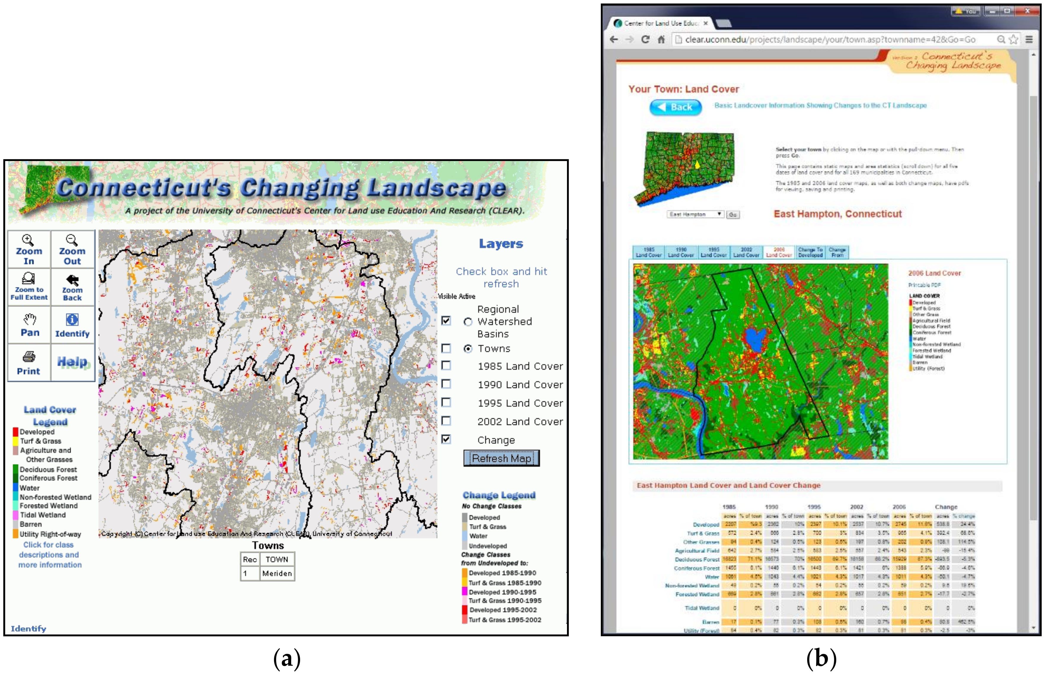
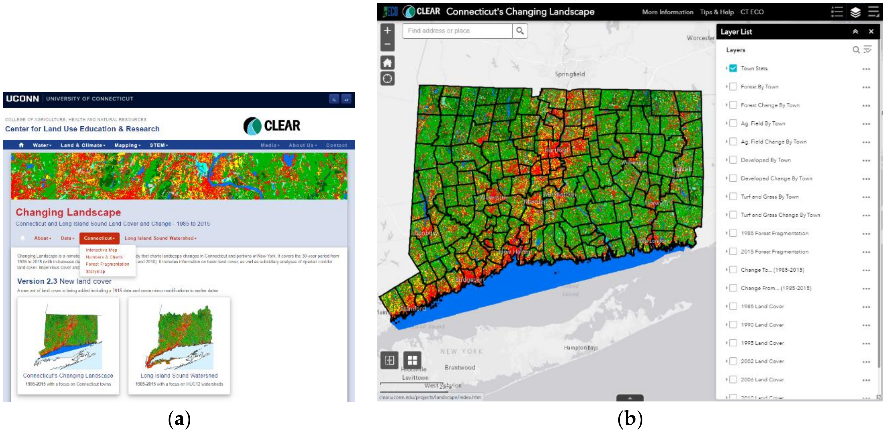
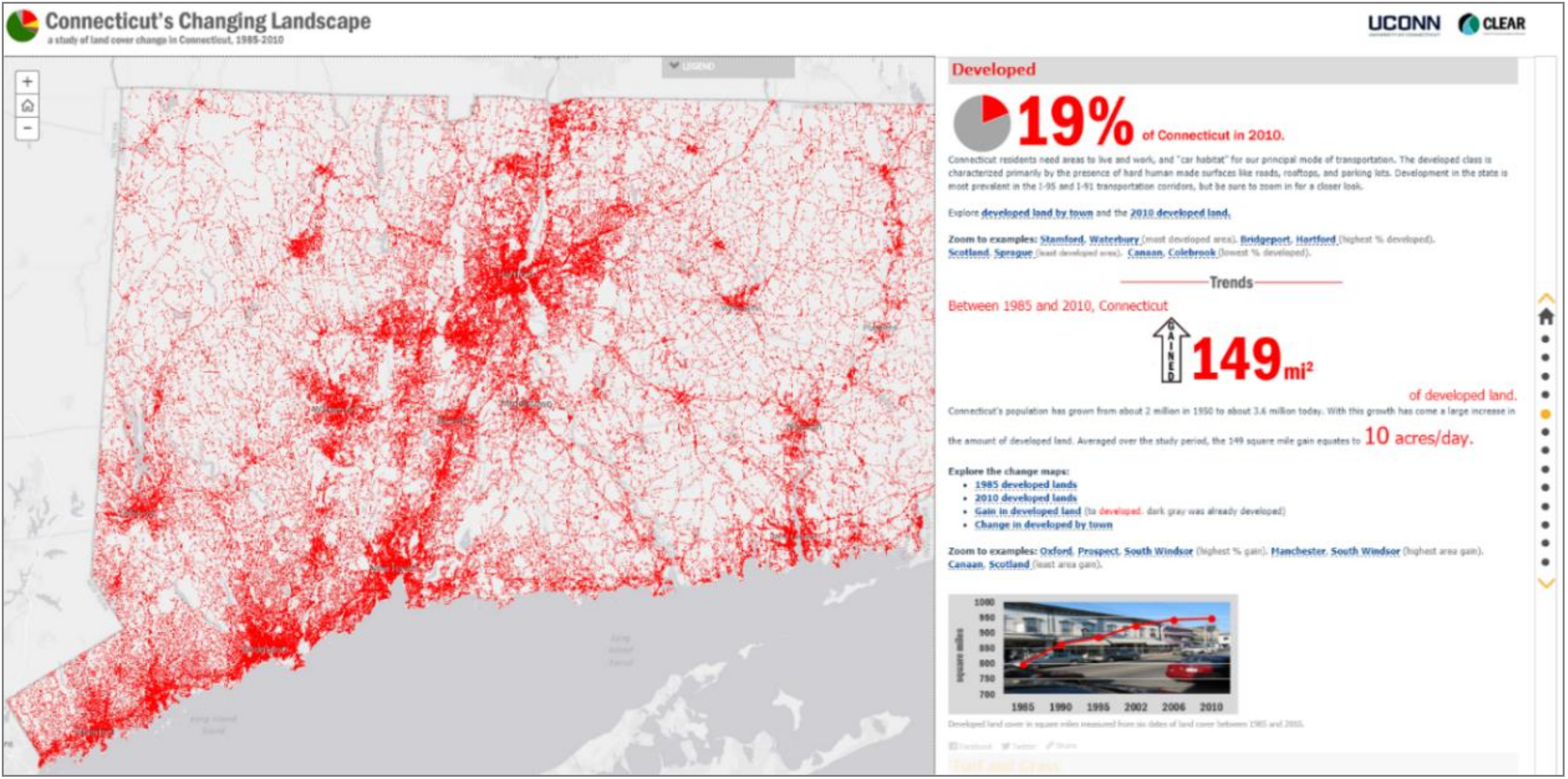
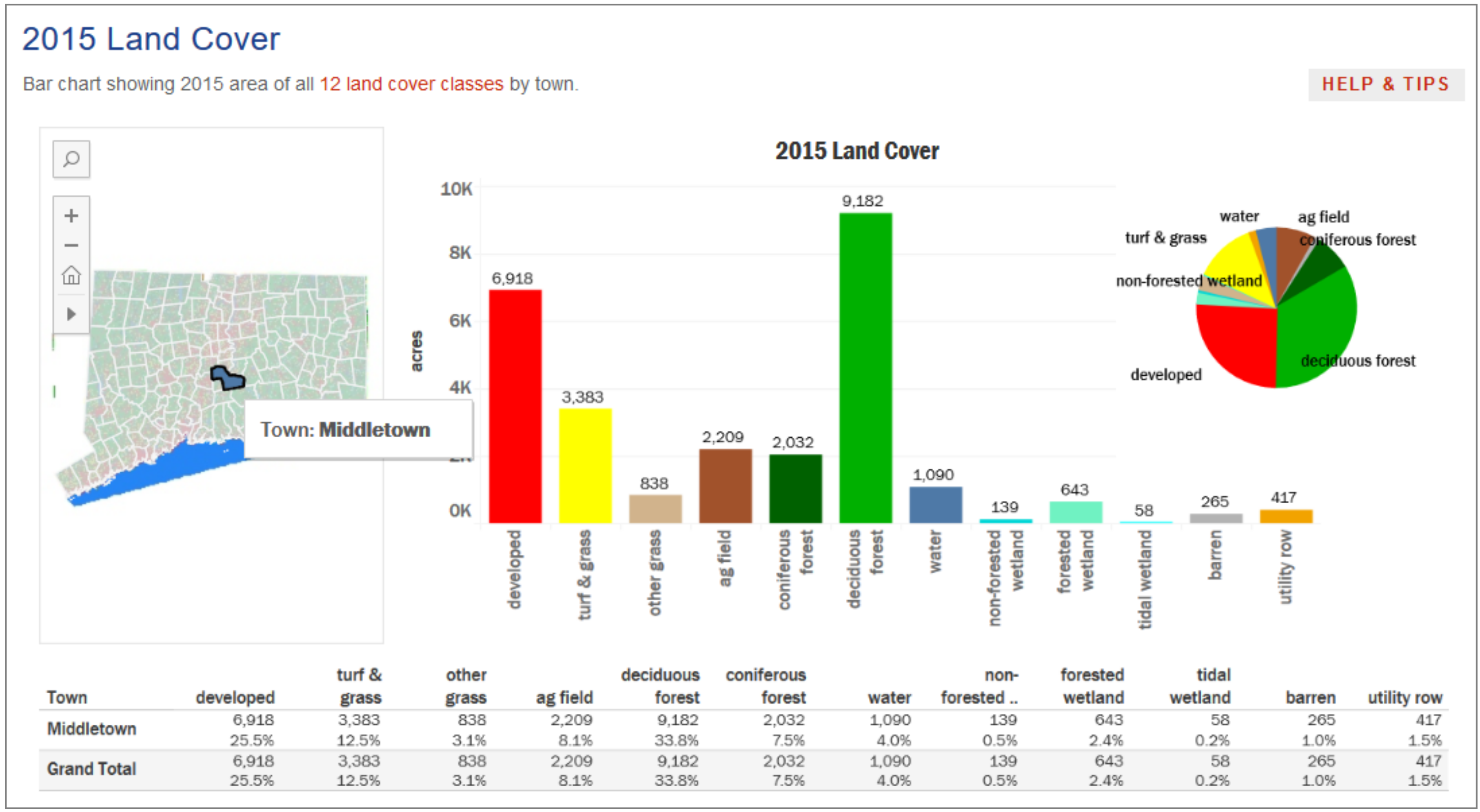
4. Results: Information Dissemination

The online CCL information is accessed frequently. As noted, the first appearance of the CCL website was in 2004; however, the project did not collect reliable usage statistics for this site until 2013. Statistics generated by Google Analytics for the seven calendar years from 2013 to 2019 show that CCL was the most accessed project on the CLEAR website, with over 78,000 pageviews, about 21% of the CLEAR website total. The second most accessed project was the companion Long Island Sound Watershed Changing Landscape, with over 15,000 pageviews. The most popular sections of the CCL website were those devoted to forest fragmentation (26% of the overall project pageviews) and the Your Town/Your Watershed utility, which accounted for over 19% of the overall project pageviews, despite being discontinued at the end of 2017.

Statistics are harder to generate for the sections of the website involving interactive maps. The CCL Story Map has been accessed from its inception in June 2015 to present by more than 16,000 visitors; it also won a national award from ESRI in 2015 for Best Science/Technology/Education Story Map.

The web statistics show dissemination far beyond the small group of fellow scientists and federal/state regulators who might normally be expected to be the principal audience of a land cover research project; but how is this information being used? The project has never included a social research component to track and evaluate information of this type; however, despite this shortcoming there is ample anecdotal evidence that CCL information has been used by many sectors and at multiple levels of government.

At the local level, CCL information is often included in municipal Plans of Conservation and Development, which are required to be updated by each town every 10 years. However, perhaps the most extensive CCL use has been to support and inform state plans, policies, and regulations that in turn influence local land use decisions. CCL data on forest fragmentation and agricultural fields are used as key environmental indicators in the annual report of the Connecticut Council on Environmental Quality, an independent non-partisan body created by the state legislature in 1971 to assess the condition of Connecticut’s environment, to report its findings annually to the Governor, and recommend actions to improve state environmental programs [53]. The Connecticut state Comprehensive Open Space Acquisition Strategy, which determines the state’s priorities for protecting land and issuing grants to towns for local open space protection, uses both the overall CCL land cover change data and the agricultural fields/soils analysis [54]. The state Plan of Conservation and Development, which lays out the state’s conservation and development strategies and policies (but is not regulatory), uses the core forest areas from the CCL forest fragmentation analysis to help determine priority areas for conservation [55]. CCL core forest areas are also being used to respond to a new state law passed in 2017, which requires proposed large solar energy projects to demonstrate that they have no significant impact on core forest or important agricultural soils [56].

On the regulation side, CCL information has been used in the formulation of two state-level water quality regulations that stem from the federal Clean Water Act, referred to as Total Maximum Daily Loads (TMDLs). The riparian corridor analysis was used in the development of a statewide bacteria TMDL, and CCL riparian land cover maps and data are provided in the Appendices for each of the 180 impaired stream segments that are addressed in the regulation [57]. CCL impervious cover estimates were used in the development of the first “Impervious Cover” TMDL regulation in the nation. To support that regulation, impervious cover for 125 small (<130 square km) watersheds across the state were compared to water quality data to determine the most defensible level of impervious cover to be used as the regulatory goal [58,59]. This new “surrogate pollutant” approach has resulted in measurable results in the watershed on which it is focused [60], and although this approach has not been more broadly implemented in Connecticut, it has become a tool in other New England states [61].

Regionally, the Long Island Sound Study (LISS), a federal/state partnership that is part of the U.S. Environmental Protection Agency’s National Estuary Program, uses a geographically-extended version of CCL to help monitor progress toward key objectives. The Study issues a Comprehensive Conservation and Management Plan for the Sound that sets environmental targets and recommends actions for the federal government, the states of Connecticut and New York, and local entities. Beginning in 2005, the LISS has provided funding for several CLEAR projects that expanded the geography of CCL to include the portions of New York, Rhode Island, and Long Island (NY) that drain to the Long Island Sound; there is now a separate but largely parallel “Long Island Sound Watershed” part of the Changing Landscape website. The study uses riparian corridor information, impervious cover, and overall land cover change to help track the general status of the watershed and to assess progress toward goals related to restoration of riparian corridors and reduction of impervious surfaces [62].

5. Discussion

The data from the Connecticut’s Changing Landscape project paint a picture of a state where, over the 30 years from 1985 to 2015, forest and farmland are being replaced by development. The potential impacts of this trend on the state’s natural resource base can be discerned in both the parent study and the subsidiary analyses, perhaps more in the patterns of this growth rather than in the absolute amounts. Looking at gains in the development footprint at various levels, the data indicate a “sprawl” style of attenuated, dispersed development—a growth pattern that is often reported to have negative economic, social, and environmental impacts [63]. At the statewide level, the period from 1985–2015 saw the state’s population grow by about 12% (from 3.20 million to 3.59 million) [64], while the development footprint grew by about 21% (from 2868 km² to 3479 km²). Looking at the town level (Figure 14b), the clusters of towns experiencing the relatively greatest growth are not in the traditional transportation corridors of the major highways (I-95 and I-91), but in proximal areas in the southeast, southwest, and north. Finally, zeroing in on the local maps of new development areas, new growth is dominated in most areas by attenuated patterns as opposed to more compact patterns of growth (Figure 21). This strong evidence of suburban, largely residential development is supported by the fact that the fastest growing land cover during the study period, in relative terms, is the turf and grass category dominated by residential lawns and golf courses. Turf and grass, which increased by 26% over 1985 levels, now covers more of the state (8%) than agricultural fields (7%). This fact may or may not be significant in and of itself, but certainly has implications both culturally and for sustainability.

As far as the agricultural component of sustainability, of greatest importance is the relatively rapid new growth in the north-central portion of the state, which seems to be in direct conflict with the largest concentration of remaining agricultural lands. CCL data show that there is more developed land and much more (almost twice as much) turf and grass on prime and important agricultural soils than statewide averages, most likely due to the flat and well-drained nature of such soils, which make them attractive for residential development. Agricultural land converted to the development footprint is extremely unlikely to be available in the future for food production. However, forest is still the largest land cover on these soils, which raises the possibility of using land conservation to “bank” some of these important areas for future agricultural use.

Despite the incursions of development and the fact that Connecticut is the sixth most densely populated state in the country, it is still 58.5% forested (in 2015), a fact that has resulted in local natural resource experts saying that “never before have so many people lived among so many trees.” This situation is causing some interesting issues, as wildlife like black bear and bobcats seem to be returning to Connecticut and making use of the exurban areas [65]. However, fragmentation by roads and power lines is causing core forest to decline at a much faster rate than forest cover in general, and the overall habitat ramifications of this process have yet to be determined.

Connecticut’s extensive and ecologically important riparian areas have experienced slightly less development than statewide averages. This is likely due to a combination of factors, including a regulatory program that requires towns to review development proposals near wetlands and watercourses, and physical impediments to development (often reinforced by local zoning regulations) that include steep slopes and wet soils. More work at the individual town level, including research into the local “upland review zones” and the record of permitting decisions, is needed to tease out these factors and determine whether or not these regulatory approaches are working. In addition, new statewide land cover datasets at 10 m and 1 m resolution will soon be available for Connecticut from NOAA, enabling us to examine narrower riparian corridors with more confidence and with more direct relevance to the most commonly used local regulatory zone of 100 feet.

Further relevant to the health of the state’s water resources are the estimates of watershed imperviousness generated from the CCL land cover by the ISAT model. Unsurprisingly in light of the growth of the developed category, the 30-year record shows that impervious cover at the small watershed scale continues to mount. This has resulted in 1907 “basin” level watersheds (27% of the 7048 basins in the state) reaching imperviousness levels over 10%, a level widely demonstrated in the literature to be harmful to water quality. Reducing the amount and impact of impervious cover, largely through the use of “Low Impact Development” or “Green Stormwater Infrastructure,” has become a major focus of the state’s newly enhanced General Stormwater (“MS4”) Permit, a program of the federal Clean Water Act [66].

Our web statistics demonstrate that people are finding the CCL information, and we know that land cover information is making its way into a number of important state, regional, and local plans and regulations. This was not achieved by accident, considerable effort is needed to facilitate the connection of research to the real world. Challenges remain in this regard. One of the obstacles in successfully disseminating the information is that it is so complex: 12 land covers, 169 towns, seven study dates, and five different analyses add up to an almost unlimited number of ways to portray the data, and the danger exists of masking the central messages by drowning people in data and maps. In addition, the continually changing technology of internet interactive mapping, while opening up new possibilities for dissemination, can also be a burden in terms of the effort needed to keep current on new technologies and update websites. In general, however, advances like of development of Story Maps are enhancing researchers’ ability to “tell the story” of their work.

A summation of our findings does not, perhaps, add up to an overly optimistic prognosis for a sustainable future in Connecticut. However, it does point the way for discussions on how we might support better stewardship of our natural resources. Additionally, there are some modest successes, rooted in the dissemination half of this story. There is evidence, albeit indirect, that the longest running outreach effort using these land cover data, the NEMO program (since 1991), has resulted in changes to local land use practices. A recent CLEAR study of 85 of the state’s 169 municipalities found that all of the study towns had, to some degree, integrated the use of low impact development (LID) practices, also known as green infrastructure, into their land use plans and regulations [67]. However, since the NEMO Program has been around for nearly 30 years, this also serves to remind us that change in local land use plans, policies, and regulations is typically a very slow moving, deliberate process.

6. Conclusions

Connecticut is a wealthy state with fairly strong environmental laws but decentralized, locally-driven land use regulation and a dense population. What happens in this type of framework as development proceeds? Can federal and state environmental regulations protect natural resources and support sustainability, or will the effects of these laws be blunted by inadequate and fragmented local land use regulation? Can better land use regulation at the local level evolve quickly enough to forestall some of the greatest impacts of development on natural resources? It is difficult to see how, unless much more effort is put into science “translation” and outreach of the type we have tried to emphasize in the CCL project.

Our experience has confirmed our belief that to have the best chance for real impact on sustainability, landscape studies of this type have to expend as much time, effort, and thoughtfulness on dissemination as they do on research. Because the University of Connecticut is part of the “Land Grant” university system [68], it has a mission to develop and sustain meaningful community engagement, at least partly through the an Extension system or department [69], of which many CLEAR faculty are members. Thus, CLEAR is very much an engagement-oriented center. However, as communication, geospatial, and social media technology advances, opportunities for engaging the public need not be limited to just those who have “outreach” in their job description. As noted by the authors in 2000 [16], remote sensing and GIS can be powerful tools for outreach as well as for research; this has become even more true since that time, as the pervasive use of satellite navigation applications on computers and phones has raised the level of comfort with these technologies. Resting on this foundation, the whole gamut of new communication tools, primarily social media of all kinds (blogs, tweets, videos, Facebook, Instagram, etc.) can be brought to bear on communicating important research and/or monitoring findings to the public. In this arena, tech-savvy undergraduates and graduate students can be critical assets for the researcher wishing to connect more solidly with non-technical audiences.

Which is not to say that it is an easy task. Even simple land cover change data can become somewhat of a maze, given, for instance, relating the key messages pertaining to changes to 12 land cover categories over seven study dates and five different types of analyses. Careful consideration is needed in order to balance the need for clarity in relating key messages with the dangers of oversimplifying or losing critical content. One approach we have taken is to make our information available in multiple formats to accommodate audiences of differing degrees of technical ability, from simple pdf maps to data tables and charts to interactive maps to data download. We have applied this approach to another project, Connecticut Conditions Online, or CT ECO, which is an online, interactive repository of statewide natural resource information (Appendix A).

However, even extensive and effective outreach may not be enough. Some of our programs have evolved to providing direct assistance to Connecticut communities. Research by colleagues at the University of Connecticut has identified paucity of resources, rather than lack of will, to be the key factor in why Connecticut communities do not pursue environmental initiatives like climate adaptation planning—something the researchers have dubbed the “capacity gap” [70,71,72]. In a modest but (in our opinion) meaningful development designed to address this gap, a broad consortium of faculty at the university have developed the “Environment Corps” undergraduate program. Environment Corps classes consist of a semester class that focuses on the local impacts of, and responses to, a particular environmental problem; currently there are classes on climate change, brownfields (contaminated sites) redevelopment, and stormwater management. These classes emphasize active learning exercises such as small team projects, role playing, and field work. The following semester, students are divided into teams and work with community officials on a wide range of sustainability projects including climate resiliency plans, brownfields remediation grant proposals, green infrastructure evaluations, and a number educational initiatives. To date, 186 students have taken an Environment Corps class, completing 49 projects in 30 Connecticut municipalities.

In the end, it may be impossible to determine the exact levels, types, and locations of development that constitute the line between “sustainable” and “unsustainable.” However, targeted research can document incursions into the viability of specific natural resources such as soils, habitat, and water quality and quantity. Integrated with a concerted outreach and education effort, these studies can help to guide measures to protect and restore our critical resources. The CCL study would appear to have made a difference, both directly, by influencing change at the local level, and indirectly, by contributing to state and regional plans, regulations, and programs that intersect with local land use planning. Certainly, CCL demonstrates that even in this high-resolution world, 30-m land cover data can impact what happens on the ground at the local level.

References

1. Messina, J.P.; Pan, W.K. Different ontologies: Land change science and health research. Curr. Opin. Environ. Sustain. 2013, 5, 515–521. [Google Scholar] [CrossRef] [PubMed] [Green Version]
2. Patz, J.A.; Olson, S.H.; Uejio, C.K.; Gibbs, H.K. Disease emergence from global climate and land use change. Med. Clin. N. Am. 2008, 92, 1473–1491. [Google Scholar] [CrossRef] [PubMed]
3. Feddema, J.J.; Oleson, K.W.; Bonan, G.B.; Mearns, L.O.; Buja, L.E.; Meehl, G.A.; Washington, W.M. The importance of land-cover change in simulating future climates. Science 2005, 310, 1674–1678. [Google Scholar] [CrossRef] [PubMed] [Green Version]
4. Pielke, R.A., Sr. Land use and climate change. Science 2005, 310, 1625–1626. [Google Scholar] [CrossRef] [Green Version]
5. Stephan, P.; Ennos, R.; Golding, Y. Modeling the environmental impacts of urban land use and land cover change—A study in Merseyside, UK. 2004. Landsc. Urban Plan. 2004, 71, 295–310. [Google Scholar] [CrossRef]
6. Swenson, J.J.; Franklin, J. The effects of future urban development on habitat fragmentation in the Santa Monica Mountains. Landsc. Ecol. 2000, 15, 713–730. [Google Scholar] [CrossRef]
7. Homer, C.; Dewitz, J.; Yang, L.; Suming, J.; Danielson, P.; Xian, G.; Coulston, J.; Herold, N.; Wickham, J.; Megown, K. Completion of the 2011 National Land Cover Database for the coterminous United States-representing a decade of land cover change information. Photogramm. Eng. Remote Sens. 2015, 81, 346–354. [Google Scholar]
8. Yang, L.; Jin, S.; Danielson, P.; Homer, C.; Gass, L.; Bender, S.; Case, A.; Costello, D.; Dewitz, J.; Fry, J. A new generation of the United States National Land Cover Database: Requirements, research priorities, design, and implementation strategies. ISPRS J. Photogramm. Remote Sens. 2018, 146, 108–123. [Google Scholar] [CrossRef]
9. Nolan, J.R. Protecting the Environment through Land Use Law: Standing Ground; Environmental Law Institute: Washington, DC, USA, 2014; pp. 1–22. [Google Scholar]
10. Simis, M.J.; Madden, H.; Cacciatore, M.A.; Yeo, S.K. The lure of rationality: Why does the deficit model persist in science communication? Public Underst. Sci. 2016, 25, 400–414. [Google Scholar] [CrossRef] [Green Version]
11. Whitmer, A.; Ogden, L.; Lawton, J.; Sturner, P.; Groffman, P.; Schneider, L.; Hart, D.; Halpern, B.; Schlesinger, W.; Raciti, S. The engaged university: Providing a platform for research that transforms society. Front. Ecol. Environ. 2010, 8, 314–321. [Google Scholar] [CrossRef] [Green Version]
12. Civco, D.L.; Hurd, J.D. Multitemporal, Multisource Land Cover Mapping for the State of Connecticut. In Proceedings of the 1991 Fall Meeting of the American Society for Photogrammetry and Remote Sensing (ASPRS), Atlanta, GA, USA, 28 October–1 November 1991; pp. B141–B151. [Google Scholar]
13. Civco, D.L.; Hurd, J.D. A Hierarchical Approach to Land Use and Land Cover Mapping using Multiple Image Types. In Proceedings of the 1999 American Society for Photogrammetry and Remote Sensing (ASPRS) Annual Convention, Portland, OR, USA, 17–21 May 1999; pp. 687–698. [Google Scholar]
14. Anderson, T.H.; Taylor, G.T. Nutrient pulses, plankton blooms, and seasonal hypoxia in western Long Island Sound. Estuaries 2001, 24, 228–243. [Google Scholar] [CrossRef]
15. Stocker, J.W.; Arnold, C.; Prisloe, S.; Civco, D. Putting Geospatial Information into the Hands of the “Real” Natural Resource Managers. In Proceedings of the 1999 American Society for Photogrammetry and Remote Sensing (ASPRS) Annual Convention, Portland, OR, USA, 17–21 May 1999; pp. 1070–1076. [Google Scholar]
16. Arnold, C.L.; Civco, D.L.; Prisloe, S.; Hurd, J.D.; Stocker, J. Remote sensing-enhanced outreach education as a decision support system for local land use officials. Photogramm. Eng. Remote Sens. 2000, 66, 1251–1260. [Google Scholar]
17. Wilson, E.H.; Rozum, J.; Arnold, C. Connecticut NEMO: Multi-faceted Geospatial Support for Local Land Use Decision Makers. In Proceedings of the 2004 ASPRS Conference, Images to Decision: Remote Sensing Foundations for GIS Applications, Kansas City, MO, USA, 12–16 September 2004. [Google Scholar]
18. Hurd, J.D.; Wilson, E.H.; Civco, D.L.; Prisloe, S.; Arnold, C.L. Temporal Characterization of Connecticut’s Landscape: Methods, Results, and Applications. In Proceedings of the 2003 ASPRS Annual Convention, Anchorage, AK, USA, 2–9 May 2003. [Google Scholar]
19. Koeln, G.; Bissonnette, J. Cross-correlation Analysis: Mapping Landcover Change with a Historic Landcover Database and a Recent, Single-date Multispectral Image. In Proceedings of the 2000 ASPRS Annual Convention, Washington, DC, USA, 21–26 May 2000. [Google Scholar]
20. Smith, F.G.F.; Herold, N.; Jones, T.; Sheffield, C. Evaluation of Cross-correlation Analysis, a Semi-automated Change Detection, for Updating of an Existing Landcover Classification. In Proceedings of the 2002 ASPRS Annual Convention, Washington, DC, USA, 19–26 April 2002. [Google Scholar]
21. Wilson, E.H.; Hurd, J.D.; Civco, D.L.; Prisloe, M.P.; Arnold, C.L. Development of a geospatial model to quantify, describe and map urban growth. Remote Sens. Environ. 2003, 86, 275–285. [Google Scholar] [CrossRef]
22. USDA Natural Resources Conservation Service Soil Survey. Available online: https://www.nrcs.usda.gov/wps/portal/nrcs/main/soils/survey/ (accessed on 15 August 2019).
23. Lowrance, R.; Altier, L.S.; Newbold, J.D.; Schnabel, R.R.; Groffman, P.M.; Denver, J.M.; Correll, D.L.; Gilliam, J.W.; Robinson, J.L.; Brinsfield, R.B. Water quality functions of riparian forest buffers in Chesapeake Bay watersheds. Environ. Manag. 1997, 21, 687–712. [Google Scholar] [CrossRef]
24. Naiman, R.J.; Decamps, H. The ecology of interfaces: Riparian zones. Ann. Rev. Ecol. Syst. 1997, 28, 621–658. [Google Scholar] [CrossRef] [Green Version]
25. Gold, A.J.; Groffman, P.M.; Addy, K.; Kellogg, D.Q.; Stolt, M.; Rosenblatt, A.E. Landscape attributes as controls on ground water nitrate removal capacity of riparian zones. J. Am. Water Resour. Assoc. 2001, 37, 1457–1464. [Google Scholar] [CrossRef]
26. Mayer, P.M.; Reyonolds, S.K., Jr.; McCutchen, M.D.; Canfield, T.J. Meta-analysis of nitrogen removal in riparian buffers. J. Environ. Qual. 2007, 36, 1172–1180. [Google Scholar] [CrossRef]
27. Library of the Connecticut Department of Energy and Environmental Protection. Available online: https://www.ct.gov/deep/lib/deep/water_inland/wetlands/2014statute.pdf (accessed on 15 August 2019).
28. Bentrup, G. Conservation buffers: Design guidelines for buffers, corridors, and greenways. In General Technical Report SRS-109; Department of Agriculture, Forest Service, Southern Research Station: Asheville, NC, USA, 2008; p. 110. [Google Scholar]
29. Sweeney, B.W.; Newbold, J.D. Streamside buffer width needed to protect stream water quality, habitat and organisms: A literature review. J. Am. Water Resour. Assoc. 2014, 50, 560–584. [Google Scholar] [CrossRef]
30. Castelle, A.J.; Johnson, A.W.; Conolly, C. Wetland and stream buffer size requirements—A review. J. Environ. Qual. 1994, 23, 878–882. [Google Scholar] [CrossRef] [Green Version]
31. Wilson, E.H.; Barrett, J.; Arnold, C.L. Land cover change in the riparian corridors of Connecticut. Watershed Sci. Bull. 2011, 2, 27–33. [Google Scholar]
32. Riitters, K.H.; Wickham, J.D.; O’Neill, R.V.; Jones, K.B.; Smith, E.R. Global-scale patterns of forest fragmentation. Conserv. Ecol. 2000, 4, 1–28. [Google Scholar] [CrossRef]
33. Riitters, K.H.; Wickham, J.D.; O’Neill, R.V.; Jones, K.B.; Smith, E.R.; Coulston, J.W.; Wade, T.G.; Smith, J.H. Fragmentation of continental United States forests. Ecosystems 2002, 5, 815–822. [Google Scholar] [CrossRef]
34. Vogt, P.; Riitters, K.; Estreguil, C.; Kozak, J.; Wade, T.; Wickham, J. Mapping spatial patterns with morphological image processing. Landsc. Ecol. 2007, 22, 171–177. [Google Scholar] [CrossRef]
35. Hurd, J.D.; Wilson, E.H.; Lammey, S.G.; Civco, D.L. Characterization of Forest Fragmentation and Urban Sprawl Using Time Sequential Landsat Imagery. In Proceedings of the ASPRS 2001 Annual Convention, St. Louis, MO, USA, 23–27 April 2001. [Google Scholar]
36. Civco, D.L.; Hurd, J.D.; Wilson, E.H.; Arnold, C.L.; Prisloe, S. Quantifying and describing urbanizing landscapes in the northeast United States. Photogramm. Eng. Remote Sens. 2002, 68, 1083–1090. [Google Scholar]
37. Hurd, J.D.; Wilson, E.H.; Civco, D.L. Development of a Forest Fragmentation Index to Quantify the Rate of Forest Change. In Proceedings of the 2002 ASPRS Annual Convention, Washington, DC, USA, 19–26 April 2002. [Google Scholar]
38. Forman, R.T. Some general principles of landscape and regional ecology. Landsc. Ecol. 1995, 10, 133–142. [Google Scholar] [CrossRef]
39. Forman, R.T.; Alexander, L. Roads and their major ecological effects. Annu. Rev. Ecol. Syst. 1998, 29, 207–231. [Google Scholar] [CrossRef] [Green Version]
40. Arnold, C.L.; Gibbons, C.J. Impervious surface coverage: Emergence of a key environmental indicator. J. Am. Plan. Assoc. 1996, 62, 243–258. [Google Scholar] [CrossRef]
41. Brabec, E.; Schulte, S.; Richards, P.L. Impervious surfaces and water quality: A review of current literature and its implications for watershed planning. J. Plan. Lit. 2002, 16, 499–514. [Google Scholar] [CrossRef]
42. Schueler, T.; Fraley-McNeal, L.; Cappiella, K. Is impervious cover still important? Review of recent research. J. Hydrol. Eng. 2009, 14, 309–315. [Google Scholar] [CrossRef] [Green Version]
43. Sleavin, W.; Prisloe, S.; Giannotti, L.; Stocker, J.; Civco, D. Measuring Impervious Surfaces for Non-point Source Pollution Modeling. In Proceedings of the ASPRS 2000 Annual Convention, Washington, DC, USA, 21–26 May 2000; p. 11. [Google Scholar]
44. Prisloe, S.; Lei, Y.; Hurd, J. Interactive GIS-Based Impervious Surface Model. In Proceedings of the ASPRS 2001 Annual Convention, St. Louis, MO, USA, 23–27 April 2001. [Google Scholar]
45. Rozum, J.; Wilson, E.H.; Arnold, C.L. Strengthening integration of land use research and outreach through innovative web technology. J. Ext. 2005, 43. Available online: http://www.joe.org/joe/2005october/iw1.shtml (accessed on 4 November 2019).
46. Swift, M. Satellite Pinpoints State’s Sprawl. Hartford Courant, 4 January 2004; p. 1. [Google Scholar]
47. Arnold, C. Sprawl: A Birds-Eye View. Hartford Courant, 21 March 2004; p. 14. [Google Scholar]
48. Editorial Board. Maps Tell Sprawl Story. Hartford Courant, 22 March 2004; p. 12. [Google Scholar]
49. Clear Changing Landscape Website. Available online: http://clear.uconn.edu/projects/landscape/index.htm (accessed on 15 August 2019).
50. ESRI Story Map Website. Available online: https://storymaps.arcgis.com/ (accessed on 15 August 2019).
51. Connecticut Office of Policy and Management. The Connecticut Economy, presentation to the Connecticut Tax Study Panel. 16 September 2015. Available online: https://www.cga.ct.gov/fin/tfs%5C20140929_State%20Tax%20Panel%5C20150916/FINAL%20CT%20Economy%20-%20OPM%20Presentation.pdf (accessed on 9 July 2020).
52. Connecticut Department of Energy and Environmental Protection. Connecticut’s Inland Wetlands and Watercourses: Status and Trends Report for the Year 2010; Bureau of Water Protection and Land Reuse Inland Water Resources Division; Department of Energy and Environmental Protection: Hartford, CT, USA, 2012; Available online: https://www.ct.gov/deep/lib/deep/water_inland/wetlands/2010statusandtrendsreport.pdf (accessed on 15 August 2019).
53. Connecticut Council on Environmental Quality. Environmental Quality in Connecticut 2018. Available online: https://www.ct.gov/ceq/cwp/view.asp?a=4992&Q=605334 (accessed on 15 August 2019).
54. Connecticut Department of Energy and Environmental Protection. Comprehensive Open Space Acquisition Strategy 2016–2020 Green Plan. Available online: https://www.ct.gov/deep/lib/deep/open_space/greenplan/2016GreenPlan-CompletePlan.pdf (accessed on 15 August 2019).
55. Connecticut Office of Policy and Management. Conservation and Development Policies: The Plan for Connecticut 2018–2023. Available online: https://portal.ct.gov/-/media/OPM/IGP/ORG/cdplan/20190214--Formatted-Document--20182023-Revised-State-CD-Plan.pdf?la=en (accessed on 15 August 2019).
56. Connecticut General Legislature Website. Available online: https://www.cga.ct.gov/2017/act/pa/pdf/2017PA-00218-R00SB-00943-PA.pdf (accessed on 15 August 2019).
57. Connecticut Department of Energy and Environmental Protection. Bacteria TMDL Website. Available online: https://www.ct.gov/deep/cwp/view.asp?a=2719&q=505808&depNav_GID=1654 (accessed on 15 August 2019).
58. Bellucci, C.J. Stormwater and Aquatic Life: Making the Connection between Impervious Cover and Aquatic Life Impairments. In Proceedings of the Water Environment Federation Conference, Bellevue, WA, USA, 1–3 June 2007; pp. 1003–1018. [Google Scholar]
59. Arnold, C.L.; Bellucci, C.J.; Collins, K.; Claytor, R. Responding to the first impervious cover-based TMDL in the nation. Watershed Sci. Bull. 2010, 1, 11–18. [Google Scholar]
60. Dietz, M.E.; Arnold, C.; Milardo, K.; Miller, R. The care and feeding of a long term institutional commitment to green stormwater infrastructure: A case study at the University of Connecticut. J. Green Build. 2015, 10, 1–13. [Google Scholar] [CrossRef] [Green Version]
61. U.S. Environmental Protection Agency TMDL Website. Available online: https://www.epa.gov/tmdl/innovative-tmdls-using-impervious-cover (accessed on 15 August 2019).
62. Long Island Sound Study Website. Clean Waters and Health Watersheds Ecosystem Targets Page. Available online: http://longislandsoundstudy.net/our-vision-and-plan/clean-waters-and-healthy-watersheds/ (accessed on 15 August 2019).
63. Wilson, B.; Charkraborty, A. The environmental impacts of sprawl: Emergent themes from the past decade of planning research. Sustainability 2013, 5, 3302–3327. [Google Scholar] [CrossRef] [Green Version]
64. Statista Website. US Census Bureau Resident Population in Connecticut from 1960 to 2018 (Chart). Available online: https://www.statista.com/statistics/206104/resident-population-in-connecticut/ (accessed on 17 July 2019).
65. Evans, M.J.; Rittenhouse, T.A.G.; Hawley, J.E.; Rego, P.W. Black bear recolonization patterns on human-dominated landscapes vary based on housing: New insights from spatially explicit density models. Landsc. Urban Plan. 2017, 162, 13–24. [Google Scholar] [CrossRef] [Green Version]
66. U.S. EPA Website. Stormwater Discharges from Municipal Sources. Available online: https://www.epa.gov/npdes/stormwater-discharges-municipal-sources (accessed on 12 August 2019).
67. Dickson, D.W.; Arnold, C.L.; Dietz, M.; LeFevre, M.; Kinnear, K.; Boyer, M. The status of Low Impact Development (LID) adoption in Connecticut. Watershed Sci. Bull. 2018, 10, 1–9. [Google Scholar]
68. Mcdowell, G.R. Engaged universities: Lessons from the Land-Grant universities and Extension. Ann. Am. Acad. Polit. Soc. Sci. 2003, 585, 31–50. [Google Scholar] [CrossRef]
69. Kellogg Commission on the Future of State and Land-Grant Universities. Returning to Our Roots: The Engaged Institution; The National Association of State Universities and Land Grant Colleges: Washington, DC, USA, 1999; p. 59. Available online: http://www.aplu.org/library/returning-to-our-roots-the-engaged-institution/file (accessed on 23 February 2020).
70. Boyer, M.A.; Meinzer, M.; Bilich, A. The climate adaptation imperative: Local choices targeting global problems? Local Environ. 2017, 22, 67–85. [Google Scholar] [CrossRef]
71. Boyer, M.A. Global Climate Change and Local Action: Understanding the Connecticut Policy Trajectory. Int. Stud. Perspect. 2013, 14, 79–107. [Google Scholar] [CrossRef]
72. Barrett, J.; Hyde, B. Municipal Issues and Needs for Addressing Climate Adaptation in Connecticut. Report of the UConn Center for Land Use Education and Research and the Connecticut Sea Grant College Program. 2017, p. 23. Available online: http://clear.uconn.edu/publications/climate/Report_Municipal_Needs_Assessment_Sept_2017.pdf (accessed on 4 November 2019).
Figure 1. 2015 Connecticut’s Changing Landscape land cover map for a multi-town area, about 30 km2.
Land 09 00255 g001
Figure 2. Examples of change maps for the same region shown in Figure 1. (a) Map showing areas converted to developed (red) or turf and grass (yellow) categories during the 1985–2015 period. (b) Map showing percent of developed category, by town (darker red indicates higher percentage).
Land 09 00255 g002
Figure 3. Sample area of the riparian zone analysis that was conducted for the entire state. (a) Existing streams and waterbodies (blue) with the 91 m (300 ft) riparian zone (black); (b) includes the land cover with the streams, waterbodies, and riparian zone; (c) is just the riparian zone land cover for the example area; and (d) is the change map for the same riparian area.
Land 09 00255 g003
Figure 4. Central shoreline area of Connecticut showing forest fragmentation model results. White areas are non-forest.
Land 09 00255 g004
Figure 5. Central shoreline of Connecticut showing results of Impervious Surface Analysis Tool (ISAT) model by Hydrologic Unit Code (HUC)-12 watershed.
Land 09 00255 g005
Figure 6. Examples of maps showing (a) statewide forest cover, (b) forest area by town, and (c) forest area by HUC-12 watershed where darker greens are more forested areas than lighter greens.
Land 09 00255 g006
Figure 7. Screen captures from the original (2004) CCL website. (a) The original CCL interactive map, showing areas changed to the developed and turf and grass categories from 1985 to 2002—in this example within the context of a regional watershed. (b) The Your Town web page, in which viewers could choose their town via the state map or a pulldown menu, and generate a series of maps and a data table detailing land cover change from 1985 to 2006.
Land 09 00255 g007
Figure 8. (a) The current CCL website home page and (b) the current interactive map viewer.
Land 09 00255 g008
Figure 9. Visitors to the “Numbers and Charts” section of the CCL website can click or drag on a town or set of towns (left) and generate tailored graphs and tables relating land cover information. Shown here is the tool for the 2015 land cover data.
Land 09 00255 g009
Figure 10. The developed class “page” of the CCL Story Map, combining the interactive map on the left with text, graphics, and links on the right. Users can pan, zoom, and click on the map to view additional information.
Land 09 00255 g010
Figure 11. Breakdown of major land cover categories, statewide, 2015.
Land 09 00255 g011
Figure 12. Statewide land cover change, 1985–2015 (km2).
Land 09 00255 g012
Figure 13. Area of “development footprint” (sum of developed and turf and grass categories) over the study period from 1985 to 2015.
Land 09 00255 g013
Figure 14. For all maps (ad), darker colors represent higher percentages. (a) Percentage developed, by town, 2015, showing historical development patterns along transportation corridors Interstate 95 (coastal) and Interstate 91 (south to north). (b) Relative change in development 1985–2015, by town, showing more recent development patterns. (c) Percentage forest, by town, 2015. (d) Percentage agricultural field by town, 2015. The yellow circles highlight areas where new development is occurring in forested areas and the red square highlights the largely agricultural area in the northern river valley which is also a hot spot of new development.
Land 09 00255 g014
Figure 15. 2015 land cover distribution over prime and important agricultural soils (left) versus statewide (right).
Land 09 00255 g015
Figure 16. Forest cover versus core forest, 2015, for the whole state (a,b) and in closer detail (c,d).
Land 09 00255 g016
Figure 17. Change in total forest cover, core forest, and fragmented forest (3 categories combined) over project period.
Land 09 00255 g017
Figure 18. Impervious cover estimates for small watersheds based on 2015 land cover.
Land 09 00255 g018
Figure 19. Distribution of 7047 small watersheds in 1985 versus 2015, in terms of levels of impervious cover.
Land 09 00255 g019
Figure 20. Number of basins for each of the seven project datasets with estimated impervious cover over 10%, a level identified in the literature as commonly related to the onset of water quality problems in the receiving stream.
Land 09 00255 g020
Figure 21. A several town area showing areas changed to the developed (red) and turf and grass (yellow) categories during the study period often reveals attenuated patterns that suggest “sprawl” style suburban development.
Land 09 00255 g021