Land Use Impacts on Particulate Matter Levels in Seoul, South Korea: Comparing High and Low Seasons


Abstract
1. Introduction
2. Literature Review
3. Case Context
4. Methods
4.1. Data and Variables
4.2. Analysis
5. Results
5.1. Land Use Classification I
5.2. Land Use Classification II
6. Discussion
7. Implications and Concluding Remarks
Funding
Acknowledgments
Conflicts of Interest
References
- World Health Organization. Ambient Air Pollution: A Global Assessment of Exposure and Burden of Disease; World Health Organization: Geneva, Switzerland, 2016. [Google Scholar]
- Sicard, P.; Lesne, O.; Alexandre, N.; Mangin, A.; Collomp, R. Air quality trends and potential health effects—Development of an aggregate risk index. Atmos. Environ. 2011, 45, 1145–1153. [Google Scholar] [CrossRef]
- Kim, K.-H.; Kabir, E.; Kabir, S. A review on the human health impact of airborne particulate matter. Environ. Int. 2015, 74, 136–143. [Google Scholar] [CrossRef] [PubMed]
- Zhang, L.; Chen, X.; Xue, X.; Sun, M.; Han, B.; Li, C.; Ma, J.; Yu, H.; Sun, Z.; Zhao, L.; et al. Long-term exposure to high particulate matter pollution and cardiovascular mortality: A 12-year cohort study in four cities in northern China. Environ. Int. 2014, 62, 41–47. [Google Scholar] [CrossRef]
- Haikerwal, A.; Akram, M.; Del Monaco, A.; Smith, K.; Sim, M.R.; Meyer, M.; Tonkin, A.M.; Abramson, M.J.; Dennekamp, M. Impact of Fine Particulate Matter (PM2.5) Exposure During Wildfires on Cardiovascular Health Outcomes. J. Am. Heart Assoc. 2015, 4, e001653. [Google Scholar] [CrossRef]
- Kim, K.E.; Cho, D.; Park, H.J. Air pollution and skin diseases: Adverse effects of airborne particulate matter on various skin diseases. Life Sci. 2016, 152, 126–134. [Google Scholar] [CrossRef]
- Hamra, G.B.; Guha, N.; Cohen, A.; Laden, F.; Nielsen, R.; Samet, J.M.; Vineis, P.; Forastiere, F.; Saldiva, P.; Yorifuji, T.; et al. Outdoor Particulate Matter Exposure and Lung Cancer: A Systematic Review and Meta-Analysis. Environ. Health Perspect. 2014, 122, 906–911. [Google Scholar] [CrossRef]
- Robin, P.C.; Hart, J.E.; Yanosky, J.D.; Spiegelman, D.; Wang, M.; Fisher, J.A.; Hong, B.; Laden, F. Particulate Matter Air Pollution Exposure, Distance to Road, and Incident Lung Cancer in the Nurses’ Health Study Cohort. Environ. Health Perspect. 2014, 122, 926–932. [Google Scholar]
- Valavanidis, A.; Vlachogianni, T.; Fiotakis, K.; Loridas, S. Pulmonary Oxidative Stress, Inflammation and Cancer: Respirable Particulate Matter, Fibrous Dusts and Ozone as Major Causes of Lung Carcinogenesis through Reactive Oxygen Species Mechanisms. Int. J. Environ. Res. Public Health 2013, 10, 3886–3907. [Google Scholar] [CrossRef]
- Hu, H.; Dailey, A.B.; Kan, H.; Xu, X. The effect of atmospheric particulate matter on survival of breast cancer among US females. Breast Cancer Res Treat 2013, 139, 217–226. [Google Scholar] [CrossRef]
- Ansari, M.; Ehrampoush, M.H. Meteorological correlates and AirQ+ health risk assessment of ambient fine particulate matter in Tehran, Iran. Environ. Res. 2019, 170, 141–150. [Google Scholar] [CrossRef]
- Hung, L.-J.; Chan, T.-F.; Wu, C.-H.; Chiu, H.-F.; Yang, C.-Y. Traffic Air Pollution and Risk of Death from Ovarian Cancer in Taiwan: Fine Particulate Matter (PM2.5) as a Proxy Marker. J. Toxicol. Environ. Health Part A 2012, 75, 174–182. [Google Scholar] [CrossRef] [PubMed]
- Roy, A.; Hu, W.; Wei, F.; Korn, L.; Chapman, R.S.; Zhang, J. (Jim) Ambient particulate matter and lung function growth in Chinese children. Epidemiology 2012, 23, 464–472. [Google Scholar] [CrossRef]
- Jedrychowski, W.A.; Perera, F.P.; Spengler, J.D.; Mroz, E.; Stigter, L.; Flak, E.; Majewska, R.; Klimaszewska-Rembiasz, M.; Jacek, R. Intrauterine exposure to fine particulate matter as a risk factor for increased susceptibility to acute broncho-pulmonary infections in early childhood. Int. J. Hyg. Environ. Health 2013, 216, 395–401. [Google Scholar] [CrossRef] [PubMed]
- Karottki, D.G.; Spilak, M.; Frederiksen, M.; Jovanovic Andersen, Z.; Madsen, A.M.; Ketzel, M.; Massling, A.; Gunnarsen, L.; Møller, P.; Loft, S. Indoor and Outdoor Exposure to Ultrafine, Fine and Microbiologically Derived Particulate Matter Related to Cardiovascular and Respiratory Effects in a Panel of Elderly Urban Citizens. Int. J. Environ. Res. Public Health 2015, 12, 1667–1686. [Google Scholar] [CrossRef] [PubMed]
- Fossati, S.; Baccarelli, A.; Zanobetti, A.; Hoxha, M.; Vokonas, P.S.; Wright, R.O.; Schwartz, J. Ambient particulate air pollution and microRNAs in elderly men. Epidemiology 2014, 25, 68–78. [Google Scholar] [CrossRef] [PubMed]
- Zhu, X.; Liu, Y.; Chen, Y.; Yao, C.; Che, Z.; Cao, J. Maternal exposure to fine particulate matter (PM2.5) and pregnancy outcomes: A meta-analysis. Env. Sci Pollut Res 2015, 22, 3383–3396. [Google Scholar] [CrossRef]
- Sapkota, A.; Chelikowsky, A.P.; Nachman, K.E.; Cohen, A.J.; Ritz, B. Exposure to particulate matter and adverse birth outcomes: A comprehensive review and meta-analysis. Air Qual. Atmos. Health 2012, 5, 369–381. [Google Scholar] [CrossRef]
- Moussiopoulos, N. Air Quality in Cities; Springer Science & Business Media: Boston, NY, USA, 2013; ISBN 978-3-662-05217-4. [Google Scholar]
- Nam, K.-M.; Li, M.; Wang, Y.; Wong, K.K.H. Spatio-temporal boundary effects on pollution-health costs estimation: The case of PM2.5 pollution in Hong Kong. Int. J. Urban Sci. 2019, 23, 498–518. [Google Scholar] [CrossRef]
- Júnior, W.J.R.; Roig, H.L.; Koutrakis, P. A novel land use approach for assessment of human health: The relationship between urban structure types and cardiorespiratory disease risk. Environ. Int. 2015, 85, 334–342. [Google Scholar] [CrossRef] [PubMed]
- Honachefsky, W.B. Ecologically Based Municipal Land Use Planning; CRC Press: London, UK, 2019; ISBN 978-1-351-45392-9. [Google Scholar]
- Liu, C.; Henderson, B.H.; Wang, D.; Yang, X.; Peng, Z. A land use regression application into assessing spatial variation of intra-urban fine particulate matter (PM2.5) and nitrogen dioxide (NO2) concentrations in City of Shanghai, China. Sci. Total Environ. 2016, 565, 607–615. [Google Scholar] [CrossRef] [PubMed]
- Lee, J.-H.; Wu, C.-F.; Hoek, G.; de Hoogh, K.; Beelen, R.; Brunekreef, B.; Chan, C.-C. LUR models for particulate matters in the Taipei metropolis with high densities of roads and strong activities of industry, commerce and construction. Sci. Total Environ. 2015, 514, 178–184. [Google Scholar] [CrossRef]
- Wolf, K.; Cyrys, J.; Harciníková, T.; Gu, J.; Kusch, T.; Hampel, R.; Schneider, A.; Peters, A. Land use regression modeling of ultrafine particles, ozone, nitrogen oxides and markers of particulate matter pollution in Augsburg, Germany. Sci. Total Environ. 2017, 579, 1531–1540. [Google Scholar] [CrossRef] [PubMed]
- Ross, Z.; Jerrett, M.; Ito, K.; Tempalski, B.; Thurston, G.D. A land use regression for predicting fine particulate matter concentrations in the New York City region. Atmos. Environ. 2007, 41, 2255–2269. [Google Scholar] [CrossRef]
- Moore, D.K.; Jerrett, M.; Mack, W.J.; Künzli, N. A land use regression model for predicting ambient fine particulate matter across Los Angeles, CA. J. Environ. Monit. 2007, 9, 246–252. [Google Scholar] [CrossRef] [PubMed]
- Gulliver, J.; Morley, D.; Dunster, C.; McCrea, A.; van Nunen, E.; Tsai, M.-Y.; Probst-Hensch, N.; Eeftens, M.; Imboden, M.; Ducret-Stich, R.; et al. Land use regression models for the oxidative potential of fine particles (PM2.5) in five European areas. Environ. Res. 2018, 160, 247–255. [Google Scholar] [CrossRef] [PubMed]
- Wu, C.-D.; Chen, Y.-C.; Pan, W.-C.; Zeng, Y.-T.; Chen, M.-J.; Guo, Y.L.; Lung, S.-C.C. Land-use regression with long-term satellite-based greenness index and culture-specific sources to model PM2.5 spatial-temporal variability. Environ. Pollut. 2017, 224, 148–157. [Google Scholar] [CrossRef] [PubMed]
- Yang, H.; Chen, W.; Liang, Z. Impact of Land Use on PM2.5 Pollution in a Representative City of Middle China. Int. J. Environ. Res. Public Health 2017, 14, 462. [Google Scholar] [CrossRef]
- Henderson, S.B.; Beckerman, B.; Jerrett, M.; Brauer, M. Application of Land Use Regression to Estimate Long-Term Concentrations of Traffic-Related Nitrogen Oxides and Fine Particulate Matter. Environ. Sci. Technol. 2007, 41, 2422–2428. [Google Scholar] [CrossRef]
- Urso, P.; Cattaneo, A.; Garramone, G.; Peruzzo, C.; Cavallo, D.M.; Carrer, P. Identification of particulate matter determinants in residential homes. Build. Environ. 2015, 86, 61–69. [Google Scholar] [CrossRef]
- Yu, H.-L.; Wang, C.-H.; Liu, M.-C.; Kuo, Y.-M. Estimation of Fine Particulate Matter in Taipei Using Landuse Regression and Bayesian Maximum Entropy Methods. Int. J. Environ. Res. Public Health 2011, 8, 2153–2169. [Google Scholar] [CrossRef]
- Currie, B.A.; Bass, B. Estimates of air pollution mitigation with green plants and green roofs using the UFORE model. Urban Ecosyst 2008, 11, 409–422. [Google Scholar] [CrossRef]
- Charron, A.; Harrison, R.M. Fine (PM2.5) and Coarse (PM2.5-10) Particulate Matter on A Heavily Trafficked London Highway: Sources and Processes. Environ. Sci. Technol. 2005, 39, 7768–7776. [Google Scholar] [CrossRef]
- Pant, P.; Harrison, R.M. Estimation of the contribution of road traffic emissions to particulate matter concentrations from field measurements: A review. Atmos. Environ. 2013, 77, 78–97. [Google Scholar] [CrossRef]
- Wåhlin, P.; Berkowicz, R.; Palmgren, F. Characterisation of traffic-generated particulate matter in Copenhagen. Atmos. Environ. 2006, 40, 2151–2159. [Google Scholar] [CrossRef]
- Huang, L.; Zhang, C.; Bi, J. Development of land use regression models for PM2.5, SO2, NO2 and O3 in Nanjing, China. Environ. Res. 2017, 158, 542–552. [Google Scholar] [CrossRef]
- Hafezi, M.H.; Daisy, N.S.; Liu, L.; Millward, H. Modelling transport-related pollution emissions for the synthetic baseline population of a large Canadian university. Int. J. Urban Sci. 2019, 23, 519–533. [Google Scholar] [CrossRef]
- Amini, H.; Taghavi-Shahri, S.M.; Henderson, S.B.; Naddafi, K.; Nabizadeh, R.; Yunesian, M. Land use regression models to estimate the annual and seasonal spatial variability of sulfur dioxide and particulate matter in Tehran, Iran. Sci. Total Environ. 2014, 488–489, 343–353. [Google Scholar] [CrossRef] [PubMed]
- Hall, P.V. Seaports, Urban Sustainability, and Paradigm Shift. J. Urban Technol. 2007, 14, 87–101. [Google Scholar] [CrossRef]
- Hoek, G.; Beelen, R.; de Hoogh, K.; Vienneau, D.; Gulliver, J.; Fischer, P.; Briggs, D. A review of land-use regression models to assess spatial variation of outdoor air pollution. Atmos. Environ. 2008, 42, 7561–7578. [Google Scholar] [CrossRef]
- Ryan, P.H.; LeMasters, G.K. A Review of Land-use Regression Models for Characterizing Intraurban Air Pollution Exposure. Inhal. Toxicol. 2007, 19, 127–133. [Google Scholar] [CrossRef]
- World Health Organization WHO Global Ambient Air Quality Database (update 2018). Available online: http://www.who.int/airpollution/data/cities/en/ (accessed on 9 February 2020).
- Ministry of Environment Comprehensive Plan for Managing Particulate Matter (2020–2024). 2019. Available online: https://www.me.go.kr/home/file/readDownloadFile.do?fileId=168738&fileSeq=5 (accessed on 9 February 2020).
- Kim, H.C.; Kim, S.; Kim, B.-U.; Jin, C.-S.; Hong, S.; Park, R.; Son, S.-W.; Bae, C.; Bae, M.; Song, C.-K.; et al. Recent increase of surface particulate matter concentrations in the Seoul Metropolitan Area, Korea. Sci. Rep. 2017, 7, 1–7. [Google Scholar] [CrossRef] [PubMed]
- Seoul Metropolitan Government Reducing PM2.5 by 20 percent. Available online: https://www.seoulsolution.kr/ko/content/3514 (accessed on 11 February 2020).
- Seoul Metropolitan Government Air Quality Strategies. Available online: https://bluesky.seoul.go.kr/bluesky_notice/policy_all/inter_cooper (accessed on 11 February 2020).
- Kim, Y.; Guldmann, J.-M. Land-use regression panel models of NO2 concentrations in Seoul, Korea. Atmos. Environ. 2015, 107, 364–373. [Google Scholar] [CrossRef]
- Adam-Poupart, A.; Brand, A.; Fournier, M.; Jerrett, M. Smargiassi Spatiotemporal Modeling of Ozone Levels in Quebec (Canada): A Comparison of Kriging, Land-Use Regression (LUR), and Combined Bayesian Maximum Entropy–LUR Approaches. Environ. Health Perspect. 2014, 122, 970–976. [Google Scholar] [CrossRef] [PubMed]
- Tai, A.P.K.; Mickley, L.J.; Jacob, D.J. Correlations between fine particulate matter (PM2.5) and meteorological variables in the United States: Implications for the sensitivity of PM2.5 to climate change. Atmos. Environ. 2010, 44, 3976–3984. [Google Scholar] [CrossRef]
- Galindo, N.; Varea, M.; Gil-Moltó, J.; Yubero, E.; Nicolás, J. The Influence of Meteorology on Particulate Matter Concentrations at an Urban Mediterranean Location. Water Air Soil Pollut 2011, 215, 365–372. [Google Scholar] [CrossRef]
- Yáñez, M.A.; Baettig, R.; Cornejo, J.; Zamudio, F.; Guajardo, J.; Fica, R. Urban airborne matter in central and southern Chile: Effects of meteorological conditions on fine and coarse particulate matter. Atmos. Environ. 2017, 161, 221–234. [Google Scholar] [CrossRef]
- Zou, B.; Luo, Y.; Wan, N.; Zheng, Z.; Sternberg, T.; Liao, Y. Performance comparison of LUR and OK in PM 2.5 concentration mapping: A multidimensional perspective. Sci. Rep. 2015, 5, 1–7. [Google Scholar] [CrossRef]
- Mukerjee, S.; Willis, R.D.; Walker, J.T.; Hammond, D.; Norris, G.A.; Smith, L.A.; Welch, D.P.; Peters, T.M. Seasonal effects in land use regression models for nitrogen dioxide, coarse particulate matter, and gaseous ammonia in Cleveland, Ohio. Atmos. Pollut. Res. 2012, 3, 352–361. [Google Scholar] [CrossRef]
- Kim, H.; Kim, S.-N. The Seasonal and Diurnal Influence of Surrounding Land Use on Temperature: Findings from Seoul, South Korea. Sustainability 2017, 9, 1443. [Google Scholar] [CrossRef]
- Kwon, M.Y.; Lee, J.S.; Park, S. The effect of outdoor air pollutants and greenness on allergic rhinitis incidence rates: A cross-sectional study in Seoul, Korea. Int. J. Sustain. Dev. World Ecol. 2019, 26, 258–267. [Google Scholar] [CrossRef]
- Her, J.; Park, S.; Lee, J.S. The Effects of Bus Ridership on Airborne Particulate Matter (PM10) Concentrations. Sustainability 2016, 8, 636. [Google Scholar] [CrossRef]
- Zhou, C.; Chen, J.; Wang, S. Examining the effects of socioeconomic development on fine particulate matter (PM2.5) in China’s cities using spatial regression and the geographical detector technique. Sci. Total Environ. 2018, 619–620, 436–445. [Google Scholar] [CrossRef] [PubMed]
- Abdi, H. Partial least square regression (PLS regression). In Encyclopedia for Research Methods for the Social Sciences; SAGE Publications, Inc.: Thousand Oaks, CA, USA, 2003; pp. 792–805. [Google Scholar]
- Carrascal, L.M.; Galván, I.; Gordo, O. Partial least squares regression as an alternative to current regression methods used in ecology. Oikos 2009, 118, 681–690. [Google Scholar] [CrossRef]
- Sampson, P.D.; Richards, M.; Szpiro, A.A.; Bergen, S.; Sheppard, L.; Larson, T.V.; Kaufman, J.D. A regionalized national universal kriging model using Partial Least Squares regression for estimating annual PM2.5 concentrations in epidemiology. Atmos. Environ. 2013, 75, 383–392. [Google Scholar] [CrossRef] [PubMed]
- Yan, B.; Fang, N.F.; Zhang, P.C.; Shi, Z.H. Impacts of land use change on watershed streamflow and sediment yield: An assessment using hydrologic modelling and partial least squares regression. J. Hydrol. 2013, 484, 26–37. [Google Scholar] [CrossRef]
- Woldesenbet, T.A.; Elagib, N.A.; Ribbe, L.; Heinrich, J. Hydrological responses to land use/cover changes in the source region of the Upper Blue Nile Basin, Ethiopia. Sci. Total Environ. 2017, 575, 724–741. [Google Scholar] [CrossRef]
- Shawul, A.A.; Chakma, S.; Melesse, A.M. The response of water balance components to land cover change based on hydrologic modeling and partial least squares regression (PLSR) analysis in the Upper Awash Basin. J. Hydrol. Reg. Stud. 2019, 26, 100640. [Google Scholar] [CrossRef]
- Young, M.T.; Bechle, M.J.; Sampson, P.D.; Szpiro, A.A.; Marshall, J.D.; Sheppard, L.; Kaufman, J.D. Satellite-Based NO2 and Model Validation in a National Prediction Model Based on Universal Kriging and Land-Use Regression. Environ. Sci. Technol. 2016, 50, 3686–3694. [Google Scholar] [CrossRef]
- Xu, H.; Bechle, M.J.; Wang, M.; Szpiro, A.A.; Vedal, S.; Bai, Y.; Marshall, J.D. National PM2.5 and NO2 exposure models for China based on land use regression, satellite measurements, and universal kriging. Sci. Total Environ. 2019, 655, 423–433. [Google Scholar] [CrossRef]
- Liu, H.-L.; Shen, Y.-S. The Impact of Green Space Changes on Air Pollution and Microclimates: A Case Study of the Taipei Metropolitan Area. Sustainability 2014, 6, 8827–8855. [Google Scholar] [CrossRef]
- Wold, S. Exponentially weighted moving principal components analysis and projections to latent structures. Chemom. Intell. Lab. Syst. 1994, 23, 149–161. [Google Scholar] [CrossRef]
- Sung, H.; Lee, S.; Cheon, S. Operationalizing Jane Jacobs’s Urban Design Theory: Empirical Verification from the Great City of Seoul, Korea. J. Plan. Educ. Res. 2015, 35, 117–130. [Google Scholar] [CrossRef]
- Jeon, C.; Choi, M. Historical Review on the Characteristics of Specialized and Mixed Land Uses of Korean Zoning System: From Chosun Planning Ordinace of 1934 to City Planning Law of 1962. J. Korea Plan. Assoc. 2018, 53, 5–18. [Google Scholar] [CrossRef]
- Sung, H.; Go, D.; Choi, C.; Cheon, S.; Park, S. Effects of street-level physical environment and zoning on walking activity in Seoul, Korea. Land Use Policy 2015, 49, 152–160. [Google Scholar] [CrossRef]
- Kim, Y. An Analysis of Traffic Flows and Land-Use on Urban Air Pollution Concentrations Using Geographic Information System. J. Transp. Res. 2017, 24, 67–81. [Google Scholar]
- Lee, J.; Leem, J.; Kim, H.; Hwang, S.; Jung, D.; Park, M.; Kim, J.; Lee, J.; Park, N.; Kang, S. Land Use Regression Model for Assessing Exposure and Impacts of Air Pollutants in School Children. J. Korean Soc. Atmos. Environ. 2012, 28, 571–580. [Google Scholar] [CrossRef]


| Sector | PM10 | PM2.5 | ||
|---|---|---|---|---|
| Amount (kg) | Share | Amount (kg) | Share | |
| Combustion from energy industries | 6444 | 0.08% | 6444 | 0.26% |
| Combustion from non-industry sources | 204,908 | 2.39% | 157,084 | 6.22% |
| Combustion from manufacturing | 944 | 0.01% | 718 | 0.03% |
| Road transportation sources | 575,899 | 6.72% | 529,827 | 20.99% |
| Non-road transportation sources | 671,650 | 7.84% | 617,917 | 24.48% |
| Waste treatment | 14,558 | 0.17% | 11,587 | 0.46% |
| Natural sources | 39,416 | 0.46% | 35,474 | 1.41% |
| Fugitive dust | 6,946,046 | 81.05% | 1,064,636 | 42.19% |
| Combustion of biomass | 110,610 | 1.29% | 100,029 | 3.96% |
| Total | 8,570,475 | 100% | 2,523,716 | 100% |
| Variables | Summary Statistics | ||||
|---|---|---|---|---|---|
| Min. | Max. | Mean. | |||
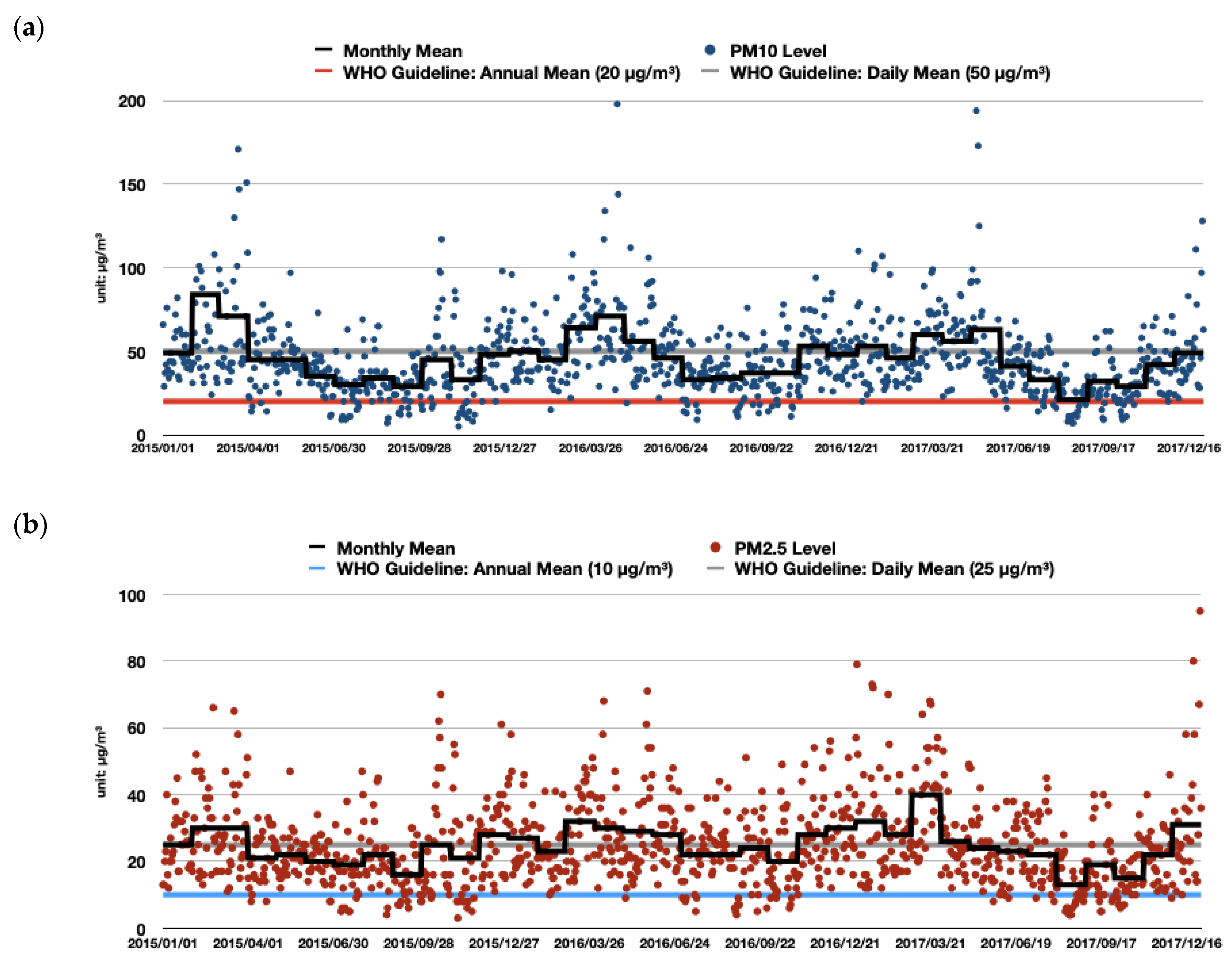
| Response variables | All seasons | Mean PM10 level (μg/m3) | 40.8 | 50.9 | 45.7 |
| Mean PM2.5 level (μg/m3) | 23.1 | 27.5 | 24.7 | ||
| High season a | Mean PM10 level (μg/m3) | 48.3 | 61.6 | 55.7 | |
| Mean PM2.5 level (μg/m3) | 26.2 | 31.9 | 28.3 | ||
| Low season b | Mean PM10 level (μg/m3) | 31.7 | 40.8 | 35.8 | |
| Mean PM2.5 level (μg/m3) | 19.1 | 23.9 | 21.1 | ||
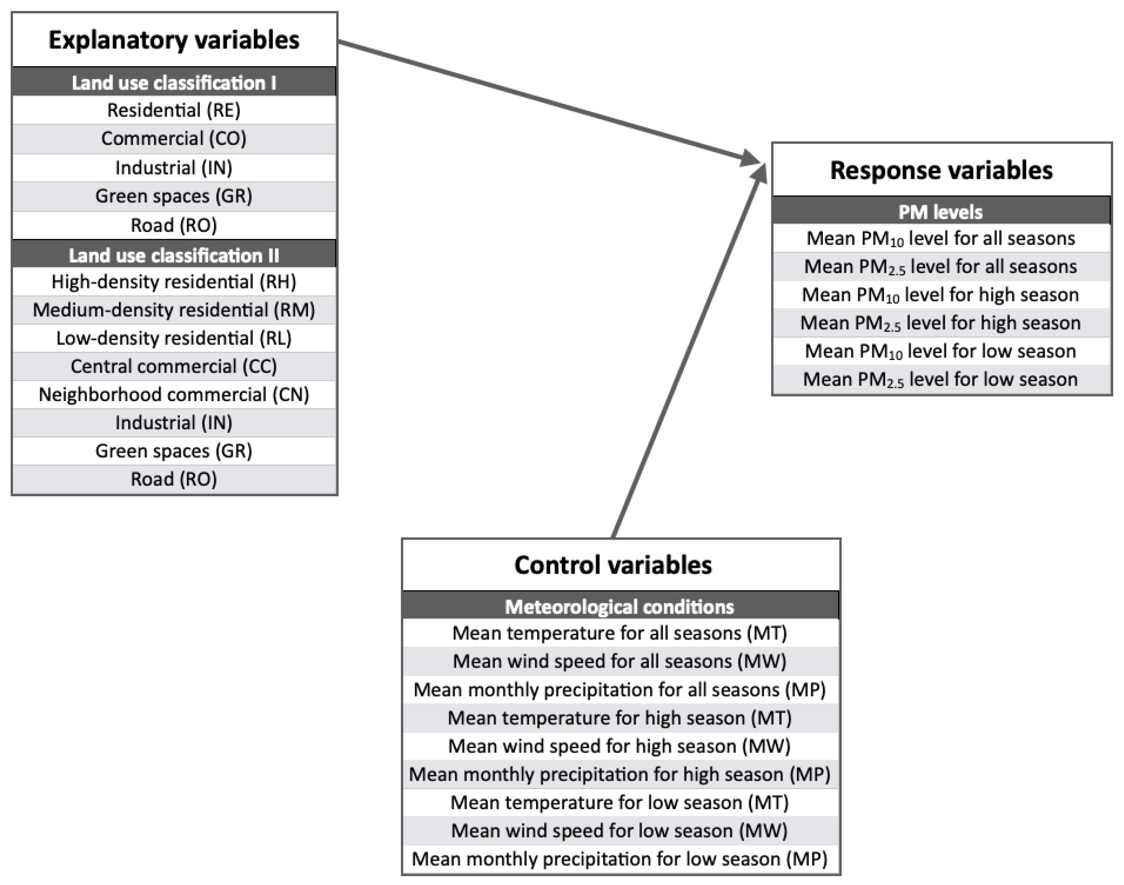
| Explanatory variables | Land use classification I | Residential (RE) (%) | 4.2 | 75.1 | 45.8 |
| Commercial (CO) (%) | 0.0 | 46.4 | 6.3 | ||
| Industrial (IN) (%) | 0.0 | 48.2 | 3.5 | ||
| Green spaces (GR) (%) | 0.0 | 55.6 | 9.1 | ||
| Road (RO) (%) | 21.0 | 49.9 | 35.3 | ||
| Land use classification II | High-density residential (RH) (%) | 3.7 | 42.3 | 17.8 | |
| Medium-density residential (RM) (%) | 0.0 | 38.8 | 20.6 | ||
| Low-density residential (RL) (%) | 0.0 | 35.6 | 6.5 | ||
| Central commercial (CC) (%) | 0.0 | 46.4 | 6.1 | ||
| Neighborhood commercial (CN) (%) | 0.0 | 1.6 | 0.1 | ||
| Industrial (IN) (%) | 0.0 | 48.2 | 3.5 | ||
| Green spaces (GR) (%) | 0.0 | 55.6 | 9.1 | ||
| Road (RO) (%) | 21.0 | 49.9 | 35.3 | ||
| Control variables | All seasons | Mean temperature (MT) (°C) | 12.0 | 14.4 | 13.6 |
| Mean wind speed (MW) (m/s) | 0.8 | 2.6 | 1.7 | ||
| Mean precipitation (MP) (mm) | 64.3 | 102.3 | 80.4 | ||
| High season a | Mean temperature (MT) (°C) | 4.8 | 7.7 | 6.8 | |
| Mean wind speed (MW) (m/s) | 0.9 | 2.7 | 1.8 | ||
| Mean precipitation (MP) (mm) | 30.3 | 43.5 | 37.8 | ||
| Low season b | Mean temperature (MT) (°C) | 18.8 | 21.1 | 20.3 | |
| Mean wind speed (MW) (m/s) | 0.8 | 2.4 | 1.6 | ||
| Mean precipitation (MP) (mm) | 98.3 | 161.1 | 123.0 | ||
| All Seasons | High Season | Low Season | |||||
|---|---|---|---|---|---|---|---|
| Coeff. | VIP | Coeff. | VIP | Coeff. | VIP | ||
| Land use types a | RE | −0.024 †† | 1.843 | −0.030 †† | 1.999 | −0.022 †† | 1.434 |
| CO | 0.000 | 0.051 | −0.001 | 0.090 | 0.000 | 0.038 | |
| IN | 0.012 †† | 1.627 | 0.010 †† | 1.202 | 0.017 †† | 1.943 | |
| GR | −0.004 | 0.692 | −0.002 | 0.337 | −0.008 †† | 1.333 | |
| RO | 0.005 | 0.139 | 0.004 | 0.090 | 0.005 | 0.120 | |
| Meteorological conditions b | MT | 0.152 †† | 1.009 | 0.070 † | 0.902 | 0.171 | 0.606 |
| MW | −0.020 | 0.632 | −0.036 | 0.951 | −0.013 | 0.338 | |
| MP | 0.018 | 0.196 | 0.107 † | 0.846 | −0.061 | 0.623 | |
| R2 | 0.277 | 0.259 | 0.305 | ||||
| All Seasons | High Season | Low Season | |||||
|---|---|---|---|---|---|---|---|
| Coeff. | VIP | Coeff. | VIP | Coeff. | VIP | ||
| Land use types a | RE | −0.002 | 0.119 | −0.003 | 0.257 | 0.000 | 0.313 |
| CO | 0.006 | 0.616 | 0.003 | 0.406 | 0.010 | 0.784 | |
| IN | 0.008 † | 0.893 | 0.004 | 0.617 | 0.012 †† | 1.084 | |
| GR | −0.005 | 0.768 | −0.003 | 0.606 | −0.009 † | 0.935 | |
| RO | −0.023 | 0.564 | −0.029 | 0.705 | −0.017 | 0.318 | |
| Meteorological conditions b | MT | 0.081 | 0.475 | 0.041 | 0.671 | 0.169 | 0.466 |
| MW | −0.074 †† | 2.097 | −0.072 †† | 2.376 | −0.089 †† | 1.867 | |
| MP | −0.116 †† | 1.131 | −0.032 | 0.323 | −0.155 †† | 1.238 | |
| R2 | 0.418 | 0.243 | 0.481 | ||||
| All Seasons | High Season | Low Season | |||||
|---|---|---|---|---|---|---|---|
| Coeff. | VIP | Coeff. | VIP | Coeff. | VIP | ||
| Land use types a | RH | −0.014 †† | 1.054 | −0.014 † | 0.975 | −0.013 † | 0.884 |
| RM | −0.014 †† | 1.615 | −0.017 †† | 1.853 | −0.013 †† | 1.324 | |
| RL | −0.010 †† | 1.539 | −0.011 †† | 1.530 | −0.011 †† | 1.443 | |
| CC | −0.001 | 0.162 | −0.002 | 0.194 | −0.001 | 0.122 | |
| CN | 0.028 †† | 1.015 | 0.029 † | 0.933 | 0.028 † | 0.872 | |
| IN | 0.010 †† | 1.488 | 0.008 †† | 1.102 | 0.014 †† | 1.885 | |
| GR | −0.003 | 0.639 | −0.002 | 0.315 | −0.007 †† | 1.106 | |
| RO | 0.004 | 0.126 | 0.003 | 0.084 | 0.004 | 0.111 | |
| Meteorological conditions b | MT | 0.118 † | 0.923 | 0.053 † | 0.827 | 0.140 | 0.588 |
| MW | −0.015 | 0.579 | −0.027 † | 0.872 | −0.010 | 0.328 | |
| MP | 0.014 | 0.179 | 0.080 | 0.776 | −0.050 | 0.605 | |
| R2 | 0.354 | 0.318 | 0.364 | ||||
| All Seasons | High Season | Low Season | |||||
|---|---|---|---|---|---|---|---|
| Coeff. | VIP | Coeff. | VIP | Coeff. | VIP | ||
| Land use types a | RH | −0.015 †† | 1.059 | −0.015 †† | 1.206 | −0.017 † | 0.882 |
| RM | 0.005 | 0.527 | 0.004 | 0.458 | 0.008 | 0.601 | |
| RL | −0.001 | 0.175 | −0.002 † | 0.928 | −0.002 | 0.192 | |
| CC | 0.005 | 0.587 | 0.002 | 0.279 | 0.009 † | 0.827 | |
| CN | 0.008 | 0.265 | 0.023 † | 0.831 | −0.004 | 0.088 | |
| IN | 0.007 † | 0.978 | 0.004 † | 0.842 | 0.011 †† | 1.204 | |
| GR | −0.005 † | 0.842 | −0.003 | 0.634 | −0.008 †† | 1.040 | |
| RO | −0.021 | 0.606 | −0.028 | 0.277 | −0.015 | 0.346 | |
| Meteorological conditions b | MT | 0.076 | 0.522 | 0.040 | 0.704 | 0.155 | 0.518 |
| MW | −0.069 †† | 2.304 | −0.070 †† | 2.491 | −0.081 †† | 2.077 | |
| MP | −0.108 †† | 1.242 | −0.031 | 0.339 | −0.142 †† | 1.378 | |
| R2 | 0.444 | 0.297 | 0.490 | ||||
© 2020 by the author. Licensee MDPI, Basel, Switzerland. This article is an open access article distributed under the terms and conditions of the Creative Commons Attribution (CC BY) license (http://creativecommons.org/licenses/by/4.0/).
Share and Cite
Kim, H. Land Use Impacts on Particulate Matter Levels in Seoul, South Korea: Comparing High and Low Seasons. Land 2020, 9, 142. https://doi.org/10.3390/land9050142
Kim H. Land Use Impacts on Particulate Matter Levels in Seoul, South Korea: Comparing High and Low Seasons. Land. 2020; 9(5):142. https://doi.org/10.3390/land9050142
Chicago/Turabian StyleKim, Hyungkyoo. 2020. "Land Use Impacts on Particulate Matter Levels in Seoul, South Korea: Comparing High and Low Seasons" Land 9, no. 5: 142. https://doi.org/10.3390/land9050142
APA StyleKim, H. (2020). Land Use Impacts on Particulate Matter Levels in Seoul, South Korea: Comparing High and Low Seasons. Land, 9(5), 142. https://doi.org/10.3390/land9050142