Soil Erosion Susceptibility Mapping in Kozetopraghi Catchment, Iran: A Mixed Approach Using Rainfall Simulator and Data Mining Techniques

 ,
, 
 and
and 
Abstract
1. Introduction
2. Materials and Methods
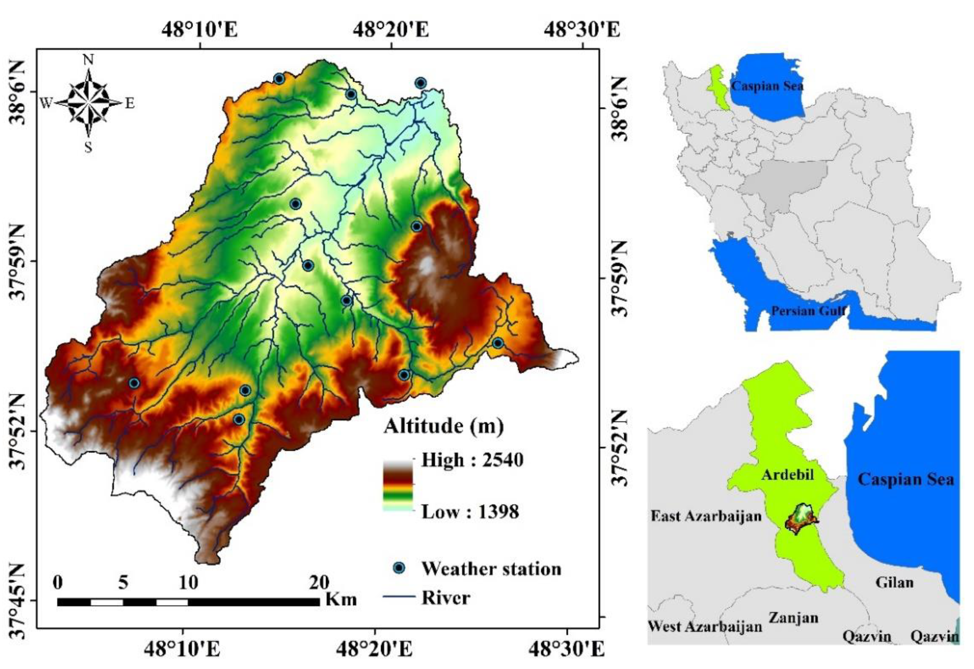
2.1. Study Area
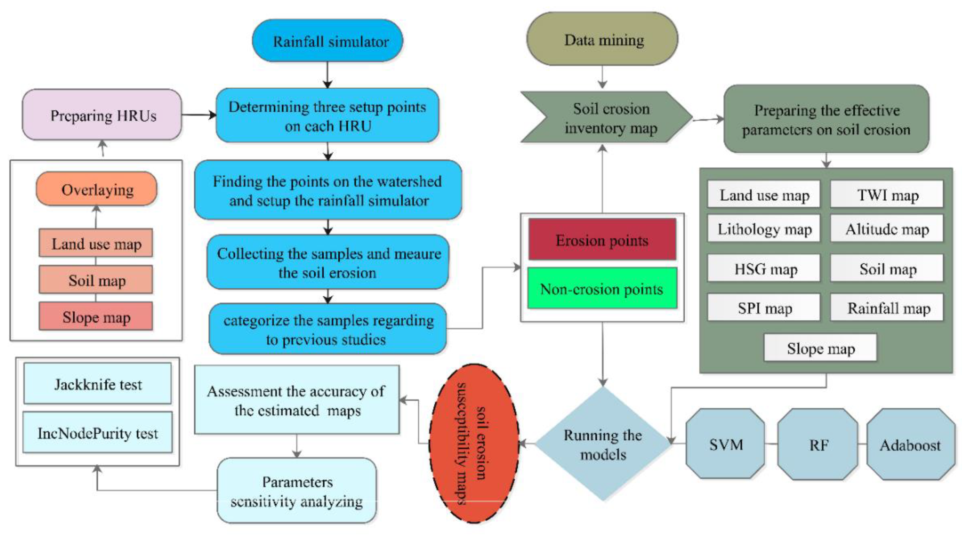
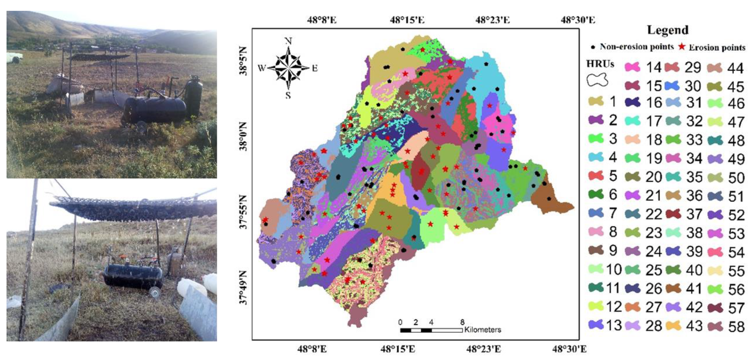
2.2. Methodology
2.3. Erosion Susceptibility Modeling
2.3.1. Support Vector Machine (SVM)
2.3.2. Random Forest (RF)
2.3.3. AdaBoost
2.4. Accuracy Assessment
2.5. Sensitivity Analysis
3. Results
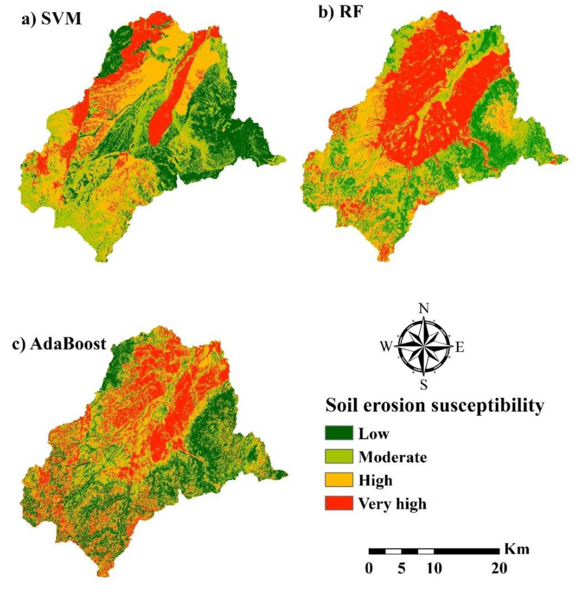
3.1. Erosion Susceptibility Mapping Results
3.2. Soil Erosion Susceptibility Classes Analyzes
3.3. Soil Erosion Plots Analysis
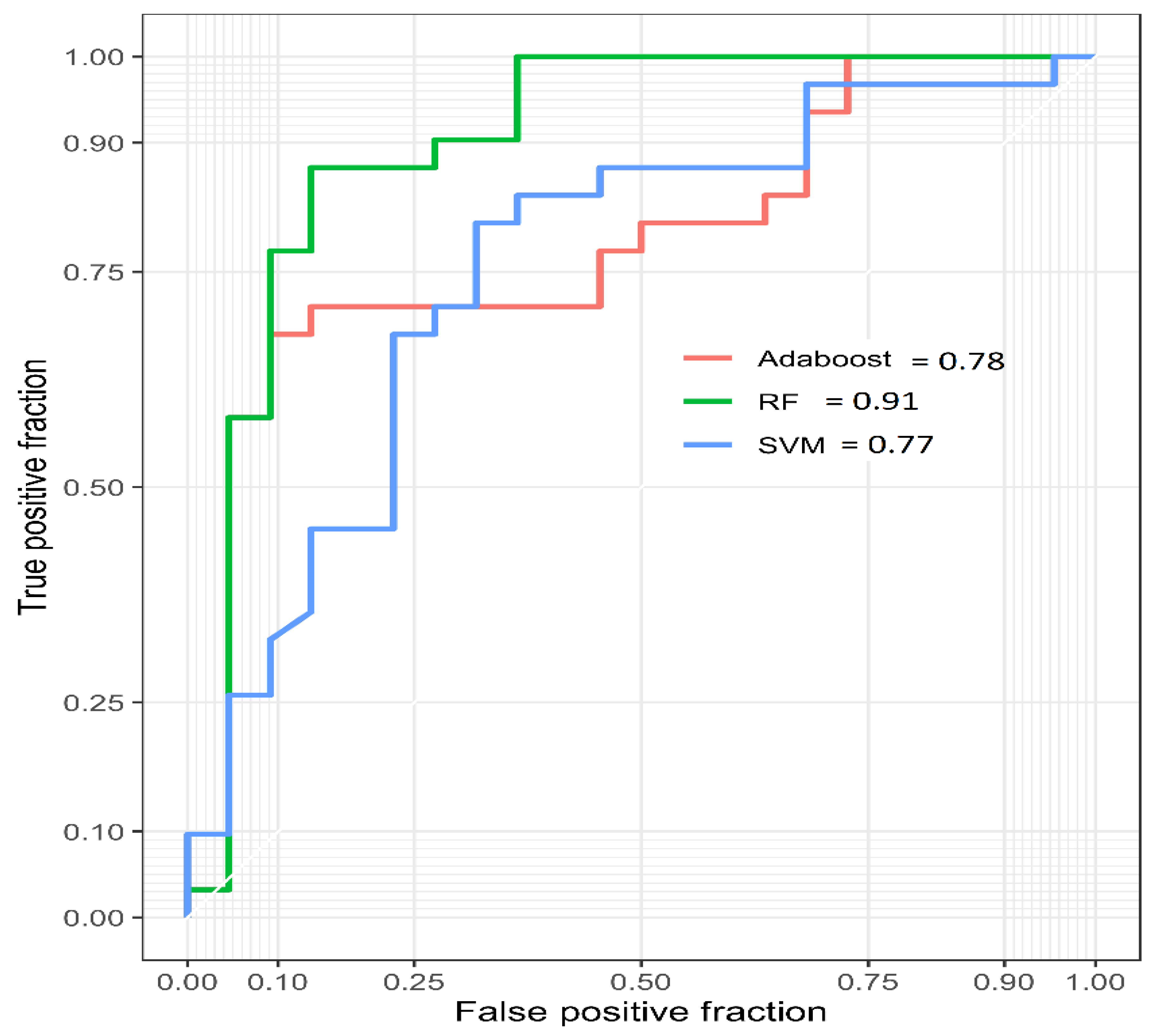
3.4. Validation of Soil Erosion Susceptibility Maps
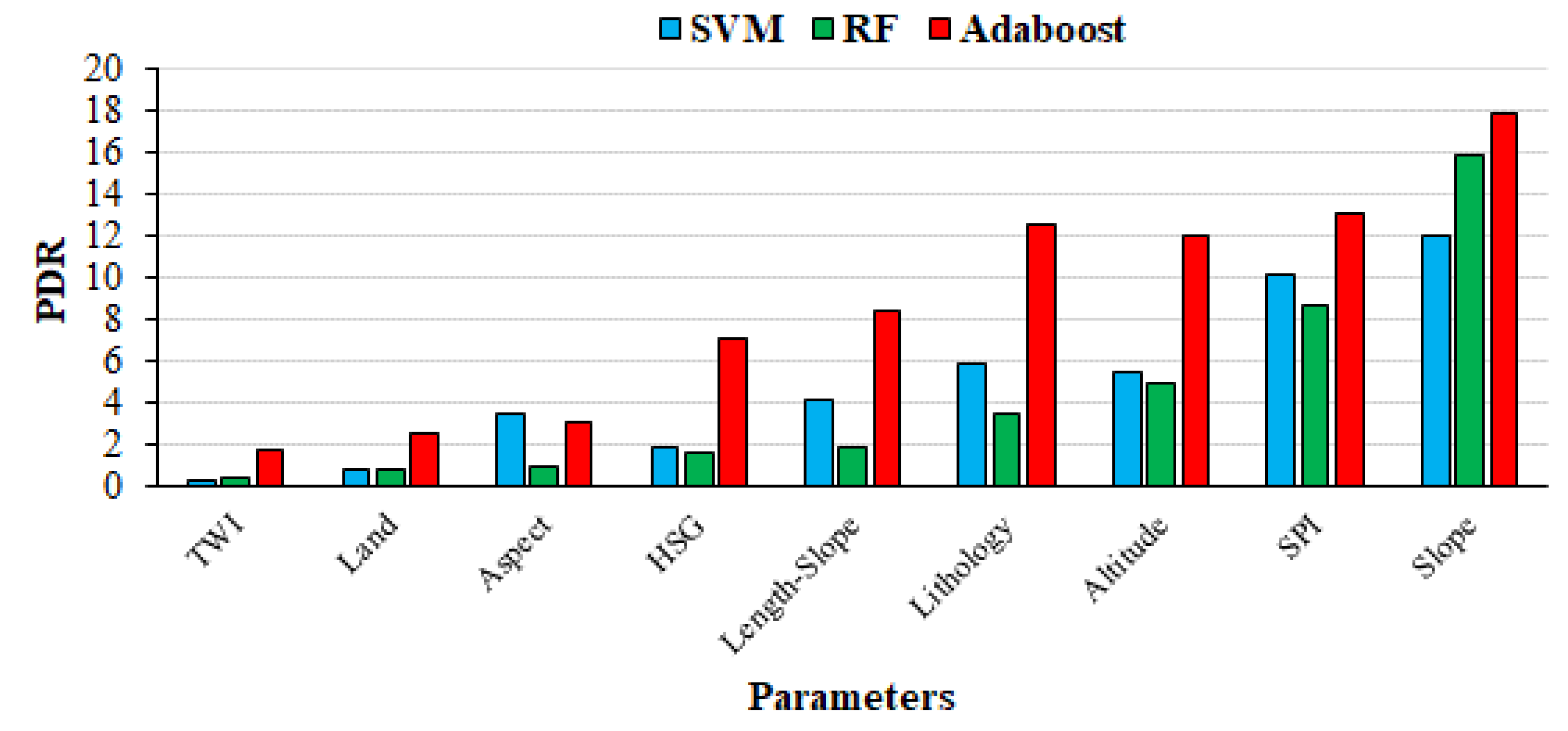
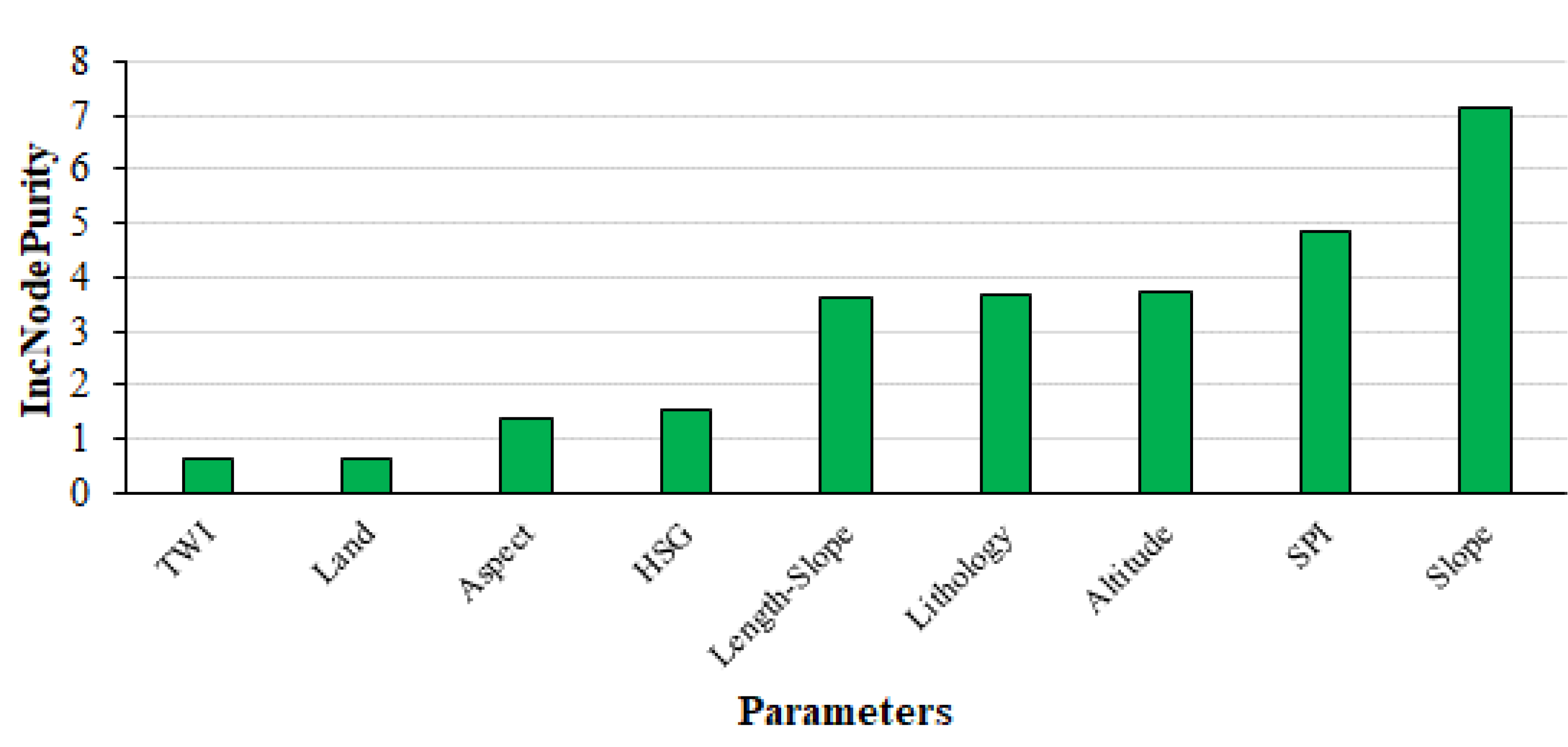
3.5. Parameters Sensitivity Analysis
4. Discussion
4.1. Spatial Variability of Soil Erosion
4.2. Soil Effect on Soil Erosion Rates
4.3. The Impact of Land Use Effect on Soil Erosion Rates
4.4. Model Outputs and Performance
4.5. Model Parameter Sensitivity
5. Conclusions
Author Contributions
Funding
Acknowledgments
Conflicts of Interest
References
- Clarke, M.L.; Rendell, H.M. Process--form relationships in Southern Italian badlands: Erosion rates and implications for landform evolution. Earth Surf. Process. Landf. J. Br. Geomorphol. Res. Gr. 2006, 31, 15–29. [Google Scholar] [CrossRef]
- Bonetti, S.; Richter, D.D.; Porporato, A. The effect of accelerated soil erosion on hillslope morphology. Earth Surf. Process. Landf. 2019, 44, 3007–3019. [Google Scholar] [CrossRef]
- Novara, A.; Stallone, G.; Cerdà, A.; Gristina, L. The effect of shallow tillage on soil erosion in a semi-arid vineyard. Agronomy 2019, 9, 257. [Google Scholar] [CrossRef]
- Cerdà, A.; Ackermann, O.; Terol, E.; Rodrigo-Comino, J. Impact of farmland abandonment on water resources and soil conservation in citrus plantations in eastern Spain. Water 2019, 11, 824. [Google Scholar] [CrossRef]
- Verity, G.E.; Anderson, D.W. Soil erosion effects on soil quality and yield. Can. J. Soil Sci. 1990, 70, 471–484. [Google Scholar] [CrossRef]
- Briassoulis, H. Combating land degradation and desertification: The land-use planning quandary. Land 2019, 8, 27. [Google Scholar] [CrossRef]
- Chalise, D.; Kumar, L.; Kristiansen, P. Land degradation by soil erosion in Nepal: A review. Soil Syst. 2019, 3, 12. [Google Scholar] [CrossRef]
- Gichenje, H.; Muñoz-Rojas, J.; Pinto-Correia, T. Opportunities and limitations for achieving land degradation-neutrality through the current land-use policy framework in Kenya. Land 2019, 8, 115. [Google Scholar] [CrossRef]
- Xie, H.; Zhang, Y.; Wu, Z.; Lv, T. A Bibliometric Analysis on Land Degradation: Current Status, Development, and Future Directions. Land 2020, 9, 28. [Google Scholar] [CrossRef]
- Keesstra, S.D. Impact of natural reforestation on floodplain sedimentation in the Dragonja basin, SW Slovenia. Earth Surf. Process. Landf. J. Br. Geomorphol. Res. Gr. 2007, 32, 49–65. [Google Scholar] [CrossRef]
- Ricci, G.F.; Jeong, J.; De Girolamo, A.M.; Gentile, F. Effectiveness and feasibility of different management practices to reduce soil erosion in an agricultural watershed. Land Use Policy 2020, 90, 104306. [Google Scholar] [CrossRef]
- Han, X.; Lv, P.; Zhao, S.; Sun, Y.; Yan, S.; Wang, M.; Han, X.; Wang, X. The Effect of the Gully Land Consolidation Project on Soil Erosion and Crop Production on a Typical Watershed in the Loess Plateau. Land 2018, 7, 113. [Google Scholar] [CrossRef]
- Woldemariam, G.W.; Iguala, A.D.; Tekalign, S.; Reddy, R.U. Spatial modeling of soil erosion risk and its implication for conservation planning: The case of the Gobele watershed, east Hararghe zone, Ethiopia. Land 2018, 7, 25. [Google Scholar] [CrossRef]
- Cerdà, A.; Keesstra, S.D.; Rodrigo-Comino, J.; Novara, A.; Pereira, P.; Brevik, E.; Giménez-Morera, A.; Fernández-Raga, M.; Pulido, M.; Di Prima, S.; et al. Runoff initiation, soil detachment and connectivity are enhanced as a consequence of vineyards plantations. J. Environ. Manag. 2017, 202, 268–275. [Google Scholar] [CrossRef]
- Khodadadi, M.; Mabit, L.; Zaman, M.; Porto, P.; Gorji, M. Using 137 Cs and 210 Pb ex measurements to explore the effectiveness of soil conservation measures in semi-arid lands: A case study in the Kouhin region of Iran. J. Soils Sediments 2019, 19, 2103–2113. [Google Scholar] [CrossRef]
- Sharpley, A.; Kleinman, P. Effect of rainfall simulator and plot scale on overland flow and phosphorus transport. J. Environ. Qual. 2003, 32, 2172–2179. [Google Scholar] [CrossRef]
- Arnaez, J.; Larrea, V.; Ortigosa, L. Surface runoff and soil erosion on unpaved forest roads from rainfall simulation tests in northeastern Spain. Catena 2004, 57, 1–14. [Google Scholar] [CrossRef]
- Wu, X.; Wei, Y.; Wang, J.; Xia, J.; Cai, C.; Wei, Z. Effects of soil type and rainfall intensity on sheet erosion processes and sediment characteristics along the climatic gradient in central-south China. Sci. Total Environ. 2018, 621, 54–66. [Google Scholar] [CrossRef]
- Keesstra, S.; Mol, G.; De Leeuw, J.; Okx, J.; De Cleen, M.; Visser, S. Soil-related sustainable development goals: Four concepts to make land degradation neutrality and restoration work. Land 2018, 7, 133. [Google Scholar] [CrossRef]
- Rodrigo-Comino, J.; Senciales González, J.M.; Cerdà Bolinches, A.; Brevik, E.C. The multidisciplinary origin of soil geography: A review. Earth Sci. Rev. 2018, 177, 114–123. [Google Scholar] [CrossRef]
- Rodrigo-Comino, J.; Davis, J.; Keesstra, S.D.; Cerdà, A. Updated measurements in vineyards improves accuracy of soil erosion rates. Agron. J. 2018, 110, 411–417. [Google Scholar] [CrossRef]
- Keesstra, S.; Pereira, P.; Novara, A.; Brevik, E.C.; Azorin-Molina, C.; Parras-Alcántara, L.; Jordán, A.; Cerdà, A. Effects of soil management techniques on soil water erosion in apricot orchards. Sci. Total Environ. 2016, 551, 357–366. [Google Scholar] [CrossRef] [PubMed]
- Kavzoglu, T.; Sahin, E.K.; Colkesen, I. Landslide susceptibility mapping using GIS-based multi-criteria decision analysis, support vector machines, and logistic regression. Landslides 2014, 11, 425–439. [Google Scholar] [CrossRef]
- Yang, R.-M.; Zhang, G.-L.; Liu, F.; Lu, Y.-Y.; Yang, F.; Yang, F.; Yang, M.; Zhao, Y.-G.; Li, D.-C. Comparison of boosted regression tree and random forest models for mapping topsoil organic carbon concentration in an alpine ecosystem. Ecol. Indic. 2016, 60, 870–878. [Google Scholar] [CrossRef]
- Moradi, H.R.; Avand, M.T.; Janizadeh, S. Landslide susceptibility survey using modeling methods. In Spatial Modeling in GIS and R for Earth and Environmental Sciences; Elsevier: Amsterdam, The Netherlands, 2019; pp. 259–276. [Google Scholar]
- Friedman, J.H. Multivariate adaptive regression splines. Ann. Stat. 1991, 19, 1–67. [Google Scholar] [CrossRef]
- Al-Abadi, A.M. Mapping flood susceptibility in an arid region of southern Iraq using ensemble machine learning classifiers: A comparative study. Arab. J. Geosci. 2018, 11, 218. [Google Scholar] [CrossRef]
- Nhu, V.-H.; Janizadeh, S.; Avand, M.; Chen, W.; Farzin, M.; Omidvar, E.; Shirzadi, A.; Shahabi, H.; Clague, J.J.; Jaafari, A.; et al. Gis-based gully erosion susceptibility mapping: A comparison of computational ensemble data mining models. Appl. Sci. 2020, 10, 2039. [Google Scholar] [CrossRef]
- Avand, M.; Janizadeh, S.; Naghibi, S.A.; Pourghasemi, H.R.; Khosrobeigi Bozchaloei, S.; Blaschke, T. A Comparative Assessment of Random Forest and k-Nearest Neighbor Classifiers for Gully Erosion Susceptibility Mapping. Water 2019, 11, 2076. [Google Scholar] [CrossRef]
- Gayen, A.; Pourghasemi, H.R.; Saha, S.; Keesstra, S.; Bai, S. Gully erosion susceptibility assessment and management of hazard-prone areas in India using different machine learning algorithms. Sci. Total Environ. 2019, 668, 124–138. [Google Scholar] [CrossRef]
- Arabameri, A.; Chen, W.; Loche, M.; Zhao, X.; Li, Y.; Lombardo, L.; Cerda, A.; Pradhan, B.; Bui, D.T. Comparison of machine learning models for gully erosion susceptibility mapping. Geosci. Front. 2019, 11, 1609–1620. [Google Scholar] [CrossRef]
- Arabameri, A.; Blaschke, T.; Pradhan, B.; Pourghasemi, H.R.; Tiefenbacher, J.P.; Bui, D.T. Evaluation of recent advanced soft computing techniques for gully erosion susceptibility mapping: A comparative study. Sensors 2020, 20, 335. [Google Scholar] [CrossRef] [PubMed]
- Pourghasemi, H.R.; Gayen, A.; Haque, S.M.; Bai, S. Gully Erosion Susceptibility Assessment Through the SVM Machine Learning Algorithm (SVM-MLA). In Gully Erosion Studies from India and Surrounding Regions; Springer: New York, NY, USA, 2020; pp. 415–425. [Google Scholar]
- Garosi, Y.; Sheklabadi, M.; Conoscenti, C.; Pourghasemi, H.R.; Van Oost, K. Assessing the performance of GIS-based machine learning models with different accuracy measures for determining susceptibility to gully erosion. Sci. Total Environ. 2019, 664, 1117–1132. [Google Scholar] [CrossRef] [PubMed]
- Hosseinalizadeh, M.; Kariminejad, N.; Alinejad, M. An application of different summary statistics for modelling piping collapses and gully headcuts to evaluate their geomorphological interactions in Golestan Province, Iran. Catena 2018, 171, 613–621. [Google Scholar] [CrossRef]
- Pereyra, M.A.; Fernández, D.S.; Marcial, E.R.; Puchulu, M.E. Agricultural land degradation by piping erosion in Chaco Plain, Northwestern Argentina. Catena 2020, 185, 104295. [Google Scholar] [CrossRef]
- Pourghasemi, H.R.; Kornejady, A.; Kerle, N.; Shabani, F. Investigating the effects of different landslide positioning techniques, landslide partitioning approaches, and presence-absence balances on landslide susceptibility mapping. Catena 2020, 187, 104364. [Google Scholar] [CrossRef]
- Ghasemain, B.; Asl, D.T.; Pham, B.T.; Avand, M.; Nguyen, H.D.; Janizadeh, S. Shallow landslide susceptibility mapping: A comparison between classification and regression tree and reduced error pruning tree algorithms. Vietnam J. Earth Sci. 2020, 42. [Google Scholar] [CrossRef]
- Van Dao, D.; Jaafari, A.; Bayat, M.; Mafi-Gholami, D.; Qi, C.; Moayedi, H.; Van Phong, T.; Ly, H.-B.; Le, T.-T.; Trinh, P.T.; et al. A spatially explicit deep learning neural network model for the prediction of landslide susceptibility. Catena 2020, 188, 104451. [Google Scholar]
- Modarres, R.; da Silva, V. de P.R. Rainfall trends in arid and semi-arid regions of Iran. J. Arid Environ. 2007, 70, 344–355. [Google Scholar] [CrossRef]
- Keshavarzi, A.; Kumar, V.; Bottega, E.L.; Rodrigo-Comino, J. Determining land management zones using pedo-geomorphological factors in potential degraded regions to achieve land degradation neutrality. Land 2019, 8, 92. [Google Scholar] [CrossRef]
- Vousoughi, F.D.; Dinpashoh, Y.; Aalami, M.T.; Jhajharia, D. Trend analysis of groundwater using non-parametric methods (case study: Ardabil plain). Stoch. Environ. Res. Risk Assess. 2013, 27, 547–559. [Google Scholar] [CrossRef]
- Kavian, A.; Golshan, M.; Abdollahi, Z. Flow discharge simulation based on land use change predictions. Environ. Earth Sci. 2017, 76, 588. [Google Scholar] [CrossRef]
- Rodrigo Comino, J.; Keesstra, S.D.; Cerdà, A. Connectivity assessment in Mediterranean vineyards using improved stock unearthing method, LiDAR and soil erosion field surveys. Earth Surf. Process. Landf. 2018, 43, 2193–2206. [Google Scholar] [CrossRef]
- Ding, Q.; Chen, W.; Hong, H. Application of frequency ratio, weights of evidence and evidential belief function models in landslide susceptibility mapping. Geocarto Int. 2017, 32, 619–639. [Google Scholar] [CrossRef]
- Choubin, B.; Moradi, E.; Golshan, M.; Adamowski, J.; Sajedi-Hosseini, F.; Mosavi, A. An ensemble prediction of flood susceptibility using multivariate discriminant analysis, classification and regression trees, and support vector machines. Sci. Total Environ. 2019, 651, 2087–2096. [Google Scholar] [CrossRef] [PubMed]
- Mathys, N.; Klotz, S.; Esteves, M.; Descroix, L.; Lapetite, J.-M. Runoff and erosion in the Black Marls of the French Alps: Observations and measurements at the plot scale. Catena 2005, 63, 261–281. [Google Scholar] [CrossRef]
- Naimi, B.; Araújo, M.B. Sdm: A reproducible and extensible R platform for species distribution modelling. Ecography 2016, 39, 368–375. [Google Scholar] [CrossRef]
- Benavides-Solorio, J.; MacDonald, L.H. Post-fire runoff and erosion from simulated rainfall on small plots, Colorado Front Range. Hydrol. Process. 2001, 15, 2931–2952. [Google Scholar] [CrossRef]
- Battany, M.C.; Grismer, M.E. Rainfall runoff and erosion in Napa Valley vineyards: Effects of slope, cover and surface roughness. Hydrol. Process. 2000, 14, 1289–1304. [Google Scholar] [CrossRef]
- Gril, J.J.; Canler, J.P.; Carsoulle, J. Benefit of permanent grass and mulching for limiting runoff and erosion in vineyards. Experimentations using rainfall-simulations in the Beaujolais. In Proceedings of the European Community Workshop on Soil Erosion Protection, Freising, Germany, 24–26 May 1988. [Google Scholar]
- Arnaez, J.; Lasanta, T.; Ruiz-Flaño, P.; Ortigosa, L. Factors affecting runoff and erosion under simulated rainfall in Mediterranean vineyards. Soil Tillage Res. 2007, 93, 324–334. [Google Scholar] [CrossRef]
- Wainwright, J. A comparison of the interrill infiltration, runoff and erosion characteristics of two contrasting badland areas in southern France. Z. Geomorphol. Suppl. 1996, 106, 183–198. [Google Scholar]
- Li, C.; Pan, C. The relative importance of different grass components in controlling runoff and erosion on a hillslope under simulated rainfall. J. Hydrol. 2018, 558, 90–103. [Google Scholar] [CrossRef]
- Dos Reis Castro, N.M.; Auzet, A.-V.; Chevallier, P.; Leprun, J.-C. Land use change effects on runoff and erosion from plot to catchment scale on the basaltic plateau of Southern Brazil. Hydrol. Process. 1999, 13, 1621–1628. [Google Scholar] [CrossRef]
- Eldridge, D.J.; Greene, R.S.B. Assessment of sediment yield by splash erosion on a semi-arid soil with varying cryptogam cover. J. Arid Environ. 1994, 26, 221–232. [Google Scholar] [CrossRef]
- Conforti, M.; Pascale, S.; Robustelli, G.; Sdao, F. Evaluation of prediction capability of the artificial neural networks for mapping landslide susceptibility in the Turbolo River catchment (northern Calabria, Italy). Catena 2014, 113, 236–250. [Google Scholar] [CrossRef]
- Sajedi-Hosseini, F.; Choubin, B.; Solaimani, K.; Cerdà, A.; Kavian, A. Spatial prediction of soil erosion susceptibility using a fuzzy analytical network process: Application of the fuzzy decision making trial and evaluation laboratory approach. L. Degrad. Dev. 2018, 29, 3092–3103. [Google Scholar] [CrossRef]
- Rachman, A.; Anderson, S.H.; Gantzer, C.J.; Thompson, A.L. Influence of long-term cropping systems on soil physical properties related to soil erodibility. Soil Sci. Soc. Am. J. 2003, 67, 637–644. [Google Scholar] [CrossRef]
- Hosseinalizadeh, M.; Kariminejad, N.; Chen, W.; Pourghasemi, H.R.; Alinejad, M.; Mohammadian Behbahani, A.; Tiefenbacher, J.P. Spatial modelling of gully headcuts using UAV data and four best-first decision classifier ensembles (BFTree, Bag-BFTree, RS-BFTree, and RF-BFTree). Geomorphology 2019, 329, 184–193. [Google Scholar] [CrossRef]
- Lucà, F.; Conforti, M.; Robustelli, G. Geomorphology Comparison of GIS-based gullying susceptibility mapping using bivariate and multivariate statistics: Northern Calabria, South Italy. Geomorphology 2011, 134, 297–308. [Google Scholar] [CrossRef]
- Mundetia, N.; Sharma, D.; Dubey, S.K. Morphometric assessment and sub-watershed prioritization of Khari River basin in semi-arid region of Rajasthan, India. Arab. J. Geosci. 2018, 11, 530. [Google Scholar] [CrossRef]
- Jahanshahi, A.; Golshan, M.; Afzali, A. Simulation of the catchments hydrological processes in arid, semi-arid and semi-humid areas. Desert 2017, 22, 1–10. [Google Scholar]
- Darabi, H.; Choubin, B.; Rahmati, O.; Haghighi, A.T.; Pradhan, B.; Kløve, B. Urban flood risk mapping using the GARP and QUEST models: A comparative study of machine learning techniques. J. Hydrol. 2019, 569, 142–154. [Google Scholar] [CrossRef]
- Olatomiwa, L.; Mekhilef, S.; Shamshirband, S.; Mohammadi, K.; Petković, D.; Sudheer, C. A support vector machine--firefly algorithm-based model for global solar radiation prediction. Sol. Energy 2015, 115, 632–644. [Google Scholar] [CrossRef]
- Breiman, L. Random Forests. Mach. Learn. 2001, 45, 5–32. [Google Scholar] [CrossRef]
- Duffy, N.; Helmbold, D. Boosting methods for regression. Mach. Learn. 2002, 47, 153–200. [Google Scholar] [CrossRef]
- Xiao, L.; Dong, Y.; Dong, Y. An improved combination approach based on Adaboost algorithm for wind speed time series forecasting. Energy Convers. Manag. 2018, 160, 273–288. [Google Scholar] [CrossRef]
- Remondo, J.; González, A.; De Terán, J.R.D.; Cendrero, A.; Fabbri, A.; Chung, C.-J.F. Validation of landslide susceptibility maps; examples and applications from a case study in Northern Spain. Nat. Hazards 2003, 30, 437–449. [Google Scholar] [CrossRef]
- Falaschi, F.; Giacomelli, F.; Federici, P.R.; Puccinelli, A.; Avanzi, G.; Pochini, A.; Ribolini, A. Logistic regression versus artificial neural networks: Landslide susceptibility evaluation in a sample area of the Serchio River valley, Italy. Nat. Hazards 2009, 50, 551–569. [Google Scholar] [CrossRef]
- Yariyan, P.; Janizadeh, S.; Van Phong, T.; Nguyen, H.D.; Costache, R.; Van Le, H.; Pham, B.T.; Pradhan, B.; Tiefenbacher, J.P. Improvement of Best First Decision Trees Using Bagging and Dagging Ensembles for Flood Probability Mapping. Water Resour. Manag. 2020, 34, 3037–3053. [Google Scholar] [CrossRef]
- Yesilnacar, E.; Topal, T. Landslide susceptibility mapping: A comparison of logistic regression and neural networks methods in a medium scale study, Hendek region (Turkey). Eng. Geol. 2005, 79, 251–266. [Google Scholar] [CrossRef]
- Falah, F.; Rahmati, O.; Rostami, M.; Ahmadisharaf, E.; Daliakopoulos, I.N.; Pourghasemi, H.R. Artificial neural networks for flood susceptibility mapping in data-scarce urban areas. In Spatial Modeling in GIS and R for Earth and Environmental Sciences; Elsevier: Amsterdam, The Netherlands, 2019; pp. 323–336. [Google Scholar]
- Nguyen, T.A.; Min, D.; Park, J.S. A comprehensive sensitivity analysis of a data center network with server virtualization for business continuity. Math. Probl. Eng. 2015, 2015. [Google Scholar] [CrossRef]
- Kaur, H.; Malhi, A.K. Ensemble Classifier to Enhance Computer Aided Diagnosis of Parkinson Disease. In Proceedings of the 2018 9th International Conference on Computing, Communication and Networking Technologies (ICCCNT), Bengaluru, India, 10–12 July 2018; pp. 1–6. [Google Scholar]
- Choubin, B.; Rahmati, O.; Tahmasebipour, N.; Feizizadeh, B.; Pourghasemi, H.R. Application of Fuzzy Analytical Network Process Model for Analyzing the Gully Erosion Susceptibility. In Natural Hazards GIS-Based Spatial Modeling Using Data Mining Techniques; Springer: New York, NY, USA, 2019; pp. 105–125. [Google Scholar]
- Wu, H. Watershed prioritization in the upper Han River basin for soil and water conservation in the South-to-North Water Transfer Project (middle route) of China. Environ. Sci. Pollut. Res. 2018, 25, 2231–2238. [Google Scholar] [CrossRef] [PubMed]
- Torabzadeh, H.; Moradi, M.; Fatehi, P. Estimating aboveground biomass in zagros forest, Iran, using sentinel-2 data. Int. Arch. Photogramm. Remote Sens. Spat. Inf. Sci. 2019, XLII-5/W2, 1059–1063. [Google Scholar] [CrossRef]
- Vahabi, J.; Nikkami, D. Assessing dominant factors affecting soil erosion using a portable rainfall simulator. Int. J. Sediment. Res. 2008, 23, 376–386. [Google Scholar] [CrossRef]
- Zhao, L.; Hou, R.; Wu, F.; Keesstra, S. Effect of soil surface roughness on infiltration water, ponding and runoff on tilled soils under rainfall simulation experiments. Soil Tillage Res. 2018, 179, 47–53. [Google Scholar] [CrossRef]
- Keesstra, S.D.; Rodrigo-Comino, J.; Novara, A.; Giménez-Morera, A.; Pulido, M.; Di Prima, S.; Cerdà, A. Straw mulch as a sustainable solution to decrease runoff and erosion in glyphosate-treated clementine plantations in Eastern Spain. An assessment using rainfall simulation experiments. Catena 2019, 174, 95–103. [Google Scholar] [CrossRef]
- Rahmati, O.; Choubin, B.; Fathabadi, A.; Coulon, F.; Soltani, E.; Shahabi, H.; Mollaefar, E.; Tiefenbacher, J.; Cipullo, S.; Ahmad, B.B.; et al. Predicting uncertainty of machine learning models for modelling nitrate pollution of groundwater using quantile regression and uneec methods. Sci. Total Environ. 2019, 688, 855–866. [Google Scholar] [CrossRef] [PubMed]
- Barrena-González, J.; Rodrigo-Comino, J.; Gyasi-Agyei, Y.; Pulido, M.; Cerdá, A. Applying the RUSLE and ISUM in the Tierra de Barros Vineyards (Extremadura, Spain) to Estimate Soil Mobilisation Rates. Land 2020, 9, 93. [Google Scholar] [CrossRef]
- Cerdà, A.; Rodrigo-Comino, J. Is the hillslope position relevant for runoff and soil loss activation under high rainfall conditions in vineyards? Ecohydrol. Hydrobiol. 2020, 20, 59–72. [Google Scholar] [CrossRef]
- Rodrigo-Comino, J.; Ponsoda-Carreres, M.; Salesa, D.; Terol, E.; Gyasi-Agyei, Y.; Cerdà, A. Soil erosion processes in subtropical plantations (Diospyros kaki) managed under flood irrigation in Eastern Spain. Singap. J. Trop. Geogr. 2020, 41, 120–135. [Google Scholar] [CrossRef]
- Cheng, Z.; Lu, D.; Li, G.; Huang, J.; Sinha, N.; Zhi, J.; Li, S. A random forest-based approach to map soil erosion risk distribution in Hickory Plantations in western Zhejiang Province, China. Remote Sens. 2018, 10, 1899. [Google Scholar] [CrossRef]
- Paul, A.; Furmanchuk, A.; Liao, W.; Choudhary, A.; Agrawal, A. Property prediction of organic donor molecules for photovoltaic applications using extremely randomized trees. Mol. Inform. 2019, 38, 1900038. [Google Scholar] [CrossRef] [PubMed]


| Region | Paper | Land Use | Slope (%) | Rainfall mm h−1 | Erosion g m−2 min−1 |
|---|---|---|---|---|---|
| Northeastern Spain | Arnáez et al. [17] | Forest roads | 5–6 | 75 | 0.4–0.5 |
| South China | Wu et al. [18] | Grass | 17.6 | 45–90 | 23.9 |
| Colorado Front Range | Benavides-Solorio & MacDonald [49] | Grass | 21 | 47 | 2 |
| Napa Valley (USA) | Battany & Grismer [50] | Range | 5.7 | 60 | 4.4 |
| Beaujolais (French) | Gril et al. [51] | Bare | 9.6 | 60 | 1.87 |
| La Rioja (Spain) | Arnaez et al. [52] | Bare | 3.4 | 70 | 0.46 |
| La Rioja (Spain) | Arnaez et al. [52] | Bare | 5 | 104 | 1.56 |
| Black Marls (French) | Mathys et al. [47] | Bare | 28.5 | 20 1 | 0.2 |
| Black Marls (French) | Mathys et al. [47] | Bare | 28.5 | 100 | 11 |
| Southeastern (French) | Wainwright [53] | Range-poor | 7.8 | 100 | 25 |
| Southeastern (French) | Wainwright [53] | Range-Good | 6.8 | 100 | 5 |
| Northern China | Li and Pan [54] | Bare | 25 | 60 | 50 |
| Northern China | Li and Pan [54] | Range | 25 | 60 | 16 |
| Southern Brazil | Dos Reis Castro et al. [55] | Agriculture | 9 | 70 | 3.2 |
| Yathong-Australia | Eldridge and Greene [56] | Range | 3 | 45 | 5.35 |
| Pennsylvania | Sharpley and Kleinman [16] | Agriculture | 0.003 | 75 | 2.64 |
| Models | Low | Moderate | High | Very High |
|---|---|---|---|---|
| Support Vector Machine (SVM) | 191 | 237 | 217 | 123 |
| Random Forest (RF) | 130 | 182 | 202 | 255 |
| Adaptive boosting (AdaBoost) | 194 | 175 | 197 | 202 |
| Models | Low | Moderate | High | Very High |
|---|---|---|---|---|
| SVM | 18 | 25 | 28 | 21 |
| RF | 5 | 20 | 27 | 40 |
| Adaboost | 11 | 23 | 25 | 33 |
| Models | Stage | Evaluation Parameters | |||||
|---|---|---|---|---|---|---|---|
| Sensitivity | Specificity | PPV | NPV | AUC | MSE | ||
| SVM | Training | 0.78 | 0.83 | 0.84 | 0.76 | 0.82 | 0.12 |
| Validation | 0.71 | 0.72 | 0.78 | 0.64 | 0.77 | 0.14 | |
| AdaBoost | Training | 0.80 | 0.86 | 0.87 | 0.79 | 0.86 | 0.11 |
| Validation | 0.71 | 0.82 | 0.85 | 0.67 | 0.78 | 0.13 | |
| RF | Training | 0.98 | 0.83 | 0.82 | 0.96 | 0.95 | 0.06 |
| Validation | 0.96 | 0.64 | 0.79 | 0.93 | 0.91 | 0.09 | |
© 2020 by the authors. Licensee MDPI, Basel, Switzerland. This article is an open access article distributed under the terms and conditions of the Creative Commons Attribution (CC BY) license (http://creativecommons.org/licenses/by/4.0/).
Share and Cite
Esmali Ouri, A.; Golshan, M.; Janizadeh, S.; Cerdà, A.; Melesse, A.M. Soil Erosion Susceptibility Mapping in Kozetopraghi Catchment, Iran: A Mixed Approach Using Rainfall Simulator and Data Mining Techniques. Land 2020, 9, 368. https://doi.org/10.3390/land9100368
Esmali Ouri A, Golshan M, Janizadeh S, Cerdà A, Melesse AM. Soil Erosion Susceptibility Mapping in Kozetopraghi Catchment, Iran: A Mixed Approach Using Rainfall Simulator and Data Mining Techniques. Land. 2020; 9(10):368. https://doi.org/10.3390/land9100368
Chicago/Turabian StyleEsmali Ouri, Abazar, Mohammad Golshan, Saeid Janizadeh, Artemi Cerdà, and Assefa M. Melesse. 2020. "Soil Erosion Susceptibility Mapping in Kozetopraghi Catchment, Iran: A Mixed Approach Using Rainfall Simulator and Data Mining Techniques" Land 9, no. 10: 368. https://doi.org/10.3390/land9100368
APA StyleEsmali Ouri, A., Golshan, M., Janizadeh, S., Cerdà, A., & Melesse, A. M. (2020). Soil Erosion Susceptibility Mapping in Kozetopraghi Catchment, Iran: A Mixed Approach Using Rainfall Simulator and Data Mining Techniques. Land, 9(10), 368. https://doi.org/10.3390/land9100368