Assessing Stormwater Nutrient and Heavy Metal Plant Uptake in an Experimental Bioretention Pond

Abstract

With the purpose to study a solution based on Sustainable Urban Drainage Systems (SUDS) to reduce and treat stormwater runoff in urban areas, a bioretention pond (BP) was realized in the Agripolis campus of the University of Padova, Italy. The BP collected overflow water volumes of the rainwater drainage system of a 2270 m² drainage area consisting almost entirely of impervious surfaces. Sixty-six Tech-IA^® floating elements, supporting four plants each, were laid on the water surface. Eleven species of herbaceous perennial helophyte plants, with ornamental features, were used and tested. The early growth results of the BP functioning showed that nearly 50% of the total inflow water volume was stored or evapotranspirated, reducing the peak discharge on the urban drainage system. Among plants, Alisma parviflora, Caltha palustris, Iris ‘Black Gamecock’, Lysimachia punctata ‘Alexander’, Oenanthe javanica ‘Flamingo’, Mentha aquatica, Phalaris arundinacea ‘Picta’, and Typha laxmannii had the best survival and growth performances. A. parviflora and M. aquatica appeared interesting also for pollutant reduction in runoff water.

1. Introduction

The high rate of urbanization has resulted in a large increase of impervious coverage in the landscape which can reach a very high percentage of the urban surface. Impervious surfaces decrease rainfall infiltration into the soil increasing runoff in terms of both peak flow and volume [1,2]. Rainwater in the urban landscape is therefore mainly directed into the municipal drainage system, creating serious problems in case of heavy rains, such as local floods, river inundations, etc., and reducing water availability and quality [3]. Urban runoff can be and often is a significant source of water pollution, causing a decline of fisheries, swimming areas, and other beneficial attributes of water resources [4]. At the same time, climate changes are causing the intensification and concentration of rainfall events, exacerbating the problem [5,6].

To reduce the problem, some environmentally sustainable approaches to urban development have been proposed as an alternative to the traditional ones to better manage the runoff in urban areas [7,8,9,10]. A stormwater best management practice (BMP) is a technique, measure, or structural control that is used to manage the quantity and improve the quality of stormwater runoff in the most cost-effective manner [11,12]. BMPs include stormwater planting, open channels, porous pavements, etc., in addition to a set of overall site design strategies and highly localized, small-scale, decentralized source control techniques, also known as Low-Impact Development (LID) systems in the USA [13,14] or Water-Sensitive Urban Design (WSUD) in Australia [15,16]. To describe stormwater technologies, such as bioretentions (including rain gardens), tree box filters, and green roofs, the term Sustainable Urban Drainage Systems (SUDS) was also coined [12,17]. SUDS may be easily integrated into buildings, infrastructure, or landscape design, taking a decentralized approach to disperse flows and manage runoff closer to where it originates, rather than controlling it downstream in a large stormwater management facility [18,19,20]. Landscape designers have the opportunity to contribute to the mitigation of the stormwater management problem, by incorporating these solutions in the design of residential gardens, corporate and institutional landscapes, and public green spaces, in order to combine aesthetic quality objectives with functional gains for the development of a more sustainable landscape [21].

More recently [22], the term Blue-Green Infrastructure (BGI) has been used to define a planned network of natural and semi-natural areas that utilize natural processes to improve water quality and manage water quantity by restoring the hydrological function of the urban landscape and managing stormwater. In particular, bioretention structures are BGIs that mimic the hydrologic function of a natural landscape providing both flood control and water quality benefits [23].

An experimental project was conducted in the Agripolis Campus of the University of Padova (Italy) in order to evaluate the efficiency in runoff reduction and water quality improvement of two bioretention solutions characterized by different scale and slightly different functions.

One solution is a rain garden system, already investigated in other environmental conditions (e.g., [24,25,26,27,28,29,30,31,32,33,34,35,36]) but not in Italy, whose research results were recently published [37,38].

The other solution is a new proposal, i.e., a bioretention pond (BP) with impervious walls to store and treat stormwater runoff as in floating treatment wetland (FTW) systems [39,40] with living ornamental plants. The BP is intended for green areas within blocks, mall centers, etc., to create a setting with aesthetic features and also able to intercept and retain stormwater runoff, reducing the peak discharge into the drainage system or main stream network, decreasing pollutants in the overflow water, and eventually working as a water reservoir for sustainable supplemental irrigation of beddings or other plant settings during drought periods. Specifically, the objective of this paper was the evaluation of the capacity of the BP to manage stormwater runoff and of the plants response in terms of growth, aesthetic quality, and potential phytoremediation. The results related to the early growth period (first two vegetative seasons) are reported.

2. Materials and Methods

The bioretention pond was set in the Agripolis Campus of the University of Padova (Figure 1), in Legnaro (45°35′ N; 11°96′ E). The area has an annual average temperature of 12.3 °C and an average minimum and maximum temperatures of −5.5 and 32.8 °C. The average annual rainfall is 811 mm, mostly distributed during the growing season, from April to November.

During Spring 2011, in proximity of a building and a parking lot of the campus, a soil area of about 70 m² was dug up to a depth of about 165 cm. With the excavation, a storage basin of about 44.5 m³ (8.10 × 5.23 m wide and 1.05 m deep) was obtained, and the entire basin was lined with a 1.5 mm thick polyolefin film.

The BP was designed to collect the overflow volumes of the existing rainwater drainage system of an area of 2270 m² consisting almost entirely of impervious surfaces (an asphalted road, sidewalks, and a building roof) (Figure 2). In fact, this drainage system has a good capacity to store and slowly let infiltrate into the soil all the runoff volumes from this area except during heavy or frequent rainfall events. The overflow volumes, which were previously discharged in a channel of the urban rainwater drainage system, were collected in a concrete sump and pumped into the BP. Water exceeding the storage capacity of the pond flowed into another sump from where it was pumped out in the channel of the local urban surface drainage system.

On July 2011, when the pond was almost full of water (102.5 mm in depth), 66 self-floating elements (Tech-IA^®, Padova, Italy), supporting four plants each, were laid down on the water surface. Tech-IA^® is a rectangular panel (0.50 × 0.90 m) produced in ethylene-vinil acetate (EVA), with eight gridded windows in which plants can be anchored. Its mass is 1732 g, and it may support a load capacity up to 20 kg [41,42]. The single elements were linked to each other, covering more than 70% of the storage basin surface (Figure 3).

The following 11 herbaceous perennial helophyte plants, with ornamental features, were used: Alisma parviflora Pursh., Bacopa caroliniana (Walt.) B.L. Robins, Caltha palustris L., Canna indica L., Iris ‘Black Gamecock’ (Louisiana Iris group), Lysimachia punctata L. ‘Alexander’, Mentha aquatica L., Oenanthe javanica Blume (DC.) ‘Flamingo’, Phalaris arundinacea L. ‘Picta’, Sagittaria sagittifolia L., and Typha laxmannii Lepech. (hereafter also called ALSSU, BAOCA, CTAPA, CNNIN, IRISS, LYSPU, MENAQ, OENJA, PHAAP, SAGSA and TYHLX, respectively according to their EPPO codes (see http://eppt.eppo.org/). For each species, six floating elements were adopted; the plants were set with the root system free in the water in three of these elements, while, in the others, the plants were set with roots confined in about 0.4 L of expanded clay, contained in plastic nets settled in place of the grids (Figure 4), through which roots could grow and reach the water.

Data collection considered the capacity of the BP in managing the overflow volumes from the existing rainwater drainage system subtracted to the canal of the urban drainage system. The inflow and outflow volumes were calculated on the basis of the operating time of the two drainage pumps (inflow pump and outflow pump) (Submersible pump MC/50-70, Pedrollo S.p.A., San Bonifacio, Italy), knowing their flow rate (1600 L min⁻¹).

The average daily actual evapotranspiration of the system was estimated in order to evaluate the capacity of the pond to ensure an adequate reservoir of water especially during dry periods. The values were calculated by measuring with a water level sensor (Levelogger Edge, Solinist Ltd., Georgetown, ON, Canada) the lowering of the water level in the pond during dry periods in different seasons. The values were compared with the average daily reference evapotranspiration ET₀ values calculated by the Penman–Monteith formula [43] using the data of the local weather station.

Samples of water were collected in the inflow and in the outflow sumps whenever the corresponding hour-counter revealed that pumps had operated. In these occasions, also three samples of water were collected from the pond at 20 cm of depth. Furthermore, samples of the BP water were collected every three weeks with no rainfall event. Water samples were analyzed for the concentration of nutrients and other ions (i.e., Cl⁻, NO³⁻, PO₄³⁻, SO₄²⁻, Na⁺, NH₄⁺, K⁺, Ca⁺, and Mg⁺), salinity, and dissolved heavy metals (i.e., Cu, Cb, Zn, and Pb). Nutrients were evaluated by means of ionic chromatography (ICS-900, Dionex, Sunnyvale, CA, USA); salinity, pH and heavy metal were determined with ICP SPECTRO CirOS Vision EOP (SPECTRO Analytical Instruments GmbH & Co., Kleve, Germany).

The plant characteristics at planting (i.e., height, leaf number, root length, dry weight) were determined in a sample of four plants per species. On November 2011, plant growth was evaluated by recording only in vivo parameters such as stem and leaf number, height, plant survival. The root growth was evaluated by means of its length and a visual rating (root visual rating RVR; 1–9 scale) based on root number and overall root growth. Furthermore, a visual rating was also adopted to evaluate the aesthetic values of the plants (aesthetic visual rating AVR; 1–9 scale) based on their potential growth in conventional condition. At the end of the second vegetative season (November 2012), the plants were evaluated as previously and, in addition, on a half of the plants, the dry weight of above-ground plant organs (AGPO) and below-ground plant organs (BGPO), comprehensive of rhizomes and stolons when present, was determined. For plants grown on substrate, the concentrations of Cd, Cu, Pb, and Zn in the dry matter were also determined, adopting [44] procedure for mineralization and ICP procedure for reading. The data were also used to calculate heavy metal content in both AGPO and BGPO, multiplying the concentrations by their respective dry weights.

The data were analyzed by mean of the analysis of variance. Statgraphics Centurion XVI software program (Statpoint Technologies, Inc., Warrenton, VA, USA) was used for data analysis. The data from the analysis of water collected in the BP were averaged before statistical analysis. The data on plant survival were analyzed by mean of the chi-square test. Non-linear regression (SigmaPlot for Windows 11.0; Systat Software, Inc., Chicago, IL, USA) was used to describe changes in nutrient concentration over time.

3. Results and Discussion

3.1. Hydrological Behaviour of the BP

During the period April 2011–November 2012, 121 rainfall events were recorded (a total of 944 mm of rain), but only 14 events generated overflow volumes from the rainwater drainage system. The total inflow volume in the BP was 245 m³, and the water volume leaving the pond as outflow was 126 m³, corresponding to 119 m³ (nearly 50% of the total inflow volume) collected or evapotranspired by the BP system. This volume was therefore subtracted from the urban stormwater drainage system, reducing the peak flow rates in the canal during rainy periods. However, it is interesting to note that only 10% of the total potential runoff volume (about 2140 m³ calculated by multiplying the drainage area for the rainfall) gave rise to overflow volume, because during the examined period the events were mostly of medium-low amount, perfectly managed by the existing rainwater drainage system.

In these occasions, the average daily evapotranspiration, calculated in no rainfall periods, was of 1.01 mm d⁻¹ during wintertime (1 December 2011–28 February 2012), 3.03 mm d⁻¹ in springtime (1 April 2012–20 May 2012), and 3.32 mm d⁻¹ in summertime (15 June 2012–25 August 2012). In the same periods, the average daily reference evapotranspiration ET₀ values calculated by the Penman–Monteith formula [43] were 0.95, 3.31, and 5.21 mm d⁻¹, respectively. The values of the actual evapotranspiration were relatively high if we consider the low transpiration of newly established plants: this was probably offset by the evaporation from the water surface left free by the floating elements (about 30% of the pond surface) and from the gridded windows without plants.

The BP was meant to guarantee a sufficient water depth for plant growth also in high-drought condition. However, even if rainfall events during the analyzed period were not frequent, the water depth in BP was high (over 100 cm deep) for most part of the experimental time. Only during summer 2012, the water level reached the lowest level (0.83 m) on 31 August. Nevertheless, as the average daily reference evapotranspiration ET₀ value during that summer was equal to 5.21 mm d⁻¹, considering a crop coefficient Kc equal to 1.2, as set for reed swamp [43] with a good plant growth, the actual ET of the system during the driest summer period could be up to 450 mm compared to the actual 285 mm that we observed. The hypothetical higher evapotranspiration would have resulted in lower depth of the storage water (about 0.60 m), which would have allowed the survival of the plants, demonstrating an adequate sizing of the BP.

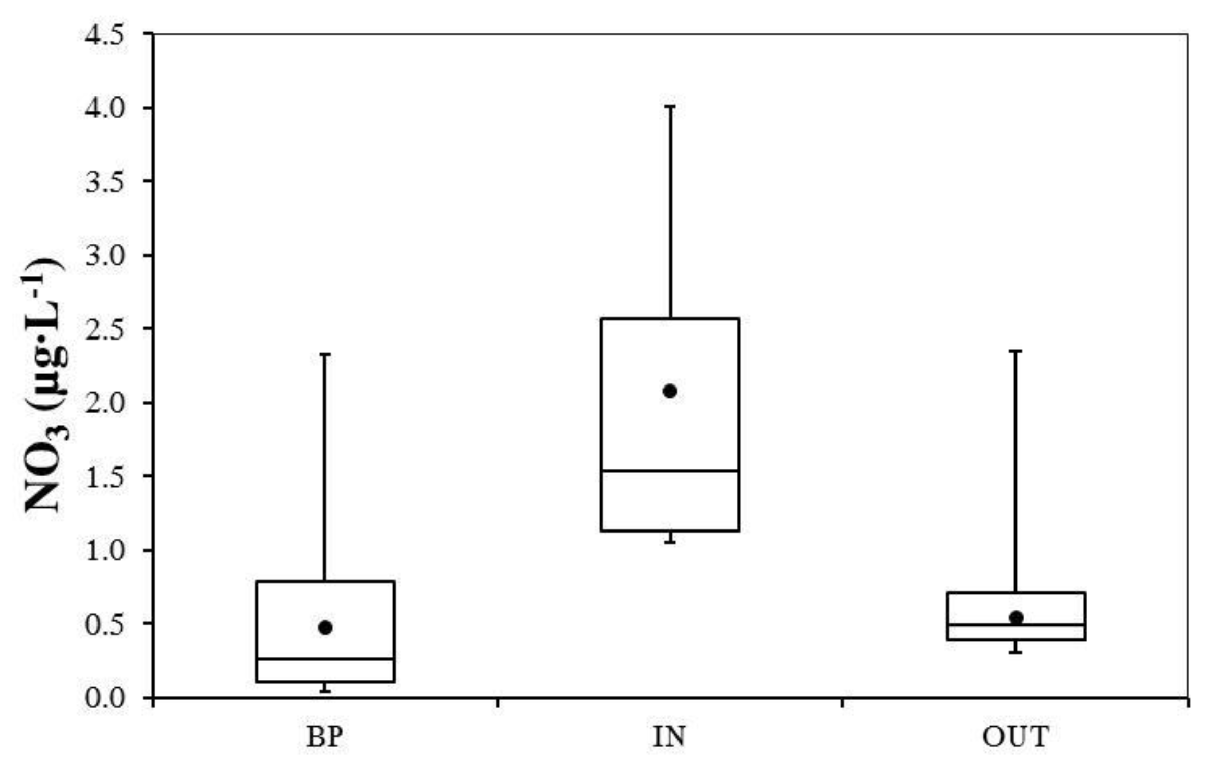
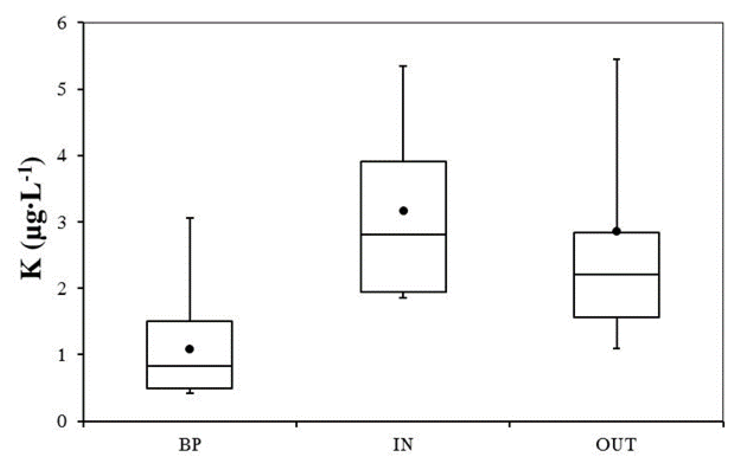
3.2. Nutrient and Heavy Metal Concentration in Stormwater

The concentrations of nutrients and other ions in the BP inflow and outflow water were in general very low. Cl⁻, Na⁺, Mg⁺, and Ca⁺ concentrations in the BP water did not change over time (on average, 0.59, 12.4, 1.30, and 11.2 mg L⁻¹, respectively), and no difference between inflow and outflow water was found.

NO₃⁻ concentration in the BP water was relatively high before plant establishment (1.53 mg L⁻¹ on average until July 2011) and, after plant establishment, it was significantly lower (on average 0.355 mg L⁻¹). From April 2012, the values were sometimes lower than the limit of instrument detection (<0.02 mg L⁻¹). Figure 5, reporting the box and whisker diagrams of nitrate concentration in the BP inflow and outflow water throughout the experimental period, highlights that the outflow water had, as expected, the same concentration as in the BP water but much lower than in the inflow water.

PO₄³⁻ concentration in water samples collected during the first growing season was low, on average 1.22 mg L⁻¹, and not always detected. In the second growing season, all samples had lower concentration values than detectable (actual sensibility of the instrument >1.0 mg L⁻¹). In contrast to what reported for NO₃⁻, no differences were noted among inflow, outflow, and BP water samples. SO₄²⁻, NH₄⁺, and K⁺ concentrations had the same pattern described for NO₃⁻, but differences resulted significant only for K⁺. As reported in Figure 6, K⁺ concentrations in inflow water were higher than those in the BP, while outflow water had intermediate values. These low values of nutrients and other ions are more comparable with those of rainwater and runoff from roofs than with those of the runoff from trafficked areas [45].

Salinity takes into account the presence of all ions in water. Salinity values did not change over time and not even differed in inflow and outflow waters (ranging from 44.7 to 89.0 µS cm⁻¹ in BP water, from 44.0 to 115 µS cm⁻¹ in inflow water, and from 54.0 to 89.0 µS cm⁻¹ in outflow water).

The water pH also did not change over time, and the values (ranging from 7.02 to 7.62) were similar to those of rainwater [45,46].

The concentrations of dissolved heavy metals in the water were in general very low and, in the case of Cd and Pb, the values were below the sensibility of the instrument (<0.001 and <0.005 mg L⁻¹, respectively). Concentrations of Cu and Zn did not apparently change over time or in inflow or outflow waters and averaged 0.007 mg L⁻¹ (range 0.002–0.012 mg L⁻¹) and 0.004 mg L⁻¹ (range 0.001–0.028 mg L⁻¹), respectively. As seen for ions, the concentrations of heavy metals were more comparable with those of rainwater and runoff from roofs than with those of the runoff from trafficked areas [45,47] or at the outlet of storm sewers [46].

The FTWs have proven to be efficient in ameliorating stormwater quality both at mesocorm experiment level [48] and at field level [41,42,49,50], leading to improvements as high as 14% for NO₃–N, 65–75% for Cu, and 40% for Zn after seven days of treatment. In the present study, the apparently low or no effect was probably due to the low concentrations of both nutrients and heavy metals in the inlet water, little surface coverage, and growth stage of the plants.

3.3. Plant Growth and Heavy Metal Accumulation

The characteristics of the plants at planting and their performance at the end of the first and second year are reported in

Table 1. Dry weight of above-ground plant organs (AGPO), below-ground plant organs (BGPO), and whole plant (WP) at the beginning and at the end of the experiment (g plant⁻¹ ± sd).

	Beginning of the Experiment	End of the Experiment			Beginning of the Experiment	End of the Experiment
		Substrate				Substrate
		No	Yes	Sig ^		No	Yes	Sig ^
	Alisma parviflora (ALSSU)				Mentha aquatic (MENAQ)
AGPO	5.37 ± 1.81	2.96	6.78	*	4.66 ± 2.12	12.8	38.6	*
BGPO	0.801 ± 0.22	2.50	4.52	*	0.633 ± 0.22	23	47.1	*
WP	6.17 ± 1.51	5.46	11.3	*	5.29 ± 2.21	35.8	85.7	*
	Bacopa caroliniana (BAOCA)				Oenanthe javanica ‘Flamingo’ (OENJA)
AGPO	0.257 ± 0.22	-	0.288		3.13 ± 0.37	-	6.32
BGPO	1.36 ± 0.32	-	0.260		0.290 ± 0.35	-	11.4
WP	1.62 ± 0.53	-	0.548		3.42 ± 0.36	-	17.7
	Canna indica (CNNIN)				Phalaris arundinacea ‘Picta’ (PHAAP)
AGPO	1.49 ± 0.57				3.05 ± 0.12	0.80	3.68	*
BGPO	1.11 ± 0.21				1.75 ± 0.14	1.32	8.77	***
WP	2.60 ± 0.66				4.80 ± 0.23	2.12	12.4	**
	Caltha palustris (CTAPA)				Sagittaria sagittifolia (SAGSA)
AGPO	4.79 ± 1.00	5.77	11.41	ns	0.501 ± 0.21	-	0.297
BGPO	9.67 ± 3.51	13.4	31.4	*	0.440 ± 0.15	-	0.548
WP	14.5 ± 3.83	19.1	42.8	*	0.941 ± 0.43	-	0.844
	Iris ‘Black Gamecock’ (IRISS)				Typha laxmannii (TYHLX)
AGPO	0.91 ± 0.19	2.34	3.65	ns	1.26 ± 0.35	4.13	11.8	*
BGPO	2.91 ± 0.96	9.38	14.8	ns	1.93 ± 1.20	2.07	11.7	*
WP	3.82 ± 1.14	11.7	18.4	ns	3.19 ± 1.55	6.2	23.5	**
	Lysimachia punctata ‘Alexander’ (LYSPU)
AGPO	1.94 ± 1.57	8.24	11.3	ns
BGPO	1.05 ± 0.94	7.18	10.9	ns
WP	2.99 ± 0.63	15.4	22.2	ns

^ ***, ** and *: significant at p ≤ 0.001, 0.01 and 0.05, respectively. ns = non-significant.

,

Table 2. Plants characteristics at the beginning of the experiment, at the end of the first year, and at the end of the second year (RVR = root visual score; AVR = aesthetic visual score).

	Beginning of the Experiment	End of the First Year			End of the Second Year
		Substrate			Substrate
		No	Yes	Sig ^	No	Yes	Sig ^
A.parviflora (ALSSU)
Stem number	1.00 ± 0.0	1.13	1.13	ns	2.27	1.75	ns
Plant height (cm)	22.4 ± 4.87	24	20.2	ns	11.6	13.4	ns
Leaf number	4.75 ± 1.86	6.1	7.2	ns	20.3	17.7	ns
Root length (cm)	3.92 ± 1.16	41.3	46.4	ns	70.4	63.2	ns
RVR (1–9 scale)		1.5	1.67	ns	4.36	2.75	ns
AVR (1–9 scale)		2.08	1.75	ns	3	2.42	ns
Mortality (%)					8.33	0.0	ns
B. caroliniana (BAOCA)
Stem number	5.96 ± 1.46	3.75	3.92	ns	-	5.25
Plant height (cm)	15.7 ± 4.6	8.08	8.92	ns	-	6.63
Root length (cm)	6.50 ± 1.93	25.0	15.3	**	-	16.1
Bud number		7.00	13.3	***
RVR (1–9 scale)		2.08	2.58	ns	-	1.38
AVR (1–9 scale)		2.58	5.10	**	-	1.38
Survival (%)		100	100	ns	0.0	66.7	***
C. indica (CNNIN)
Stem number	1.00 ± 0.0	1.17	1.67	ns
Plant height (cm)	27.9 ± 6.96	21.2	24.3	ns
Leaf number	4.17 ± 1.19	6.67	8.83	ns
Root length (cm)	6.33 ± 1.03	67.5	48.8	*
RVR (1–9 scale)		2.00	3.67	*
AVR (1–9 scale)		2.50	3.50	ns
Survival (%)		100	100	ns	0.0	0.0	ns
C. palustris (CTAPA)
Stem number	3.10 ± 1.41	2.33	3.58	**	4.50	7.75	ns
Plant height (cm)	14.2 ± 1.56	4.58	11.0	***	30.5	65.5	*
Leaf number	4.2 ± 1.92	2.50	6.58	***	10.2	16.9	ns
Root length (cm)	11.7 ± 1.10	28.7	20.7	***	50.9	68.6	*
RVR (1–9 scale)		3.50	4.50	*	4.40	7.75	ns
AVR (1–9 scale)		1.92	4.08	**	3.20	5.25	*
Survival (%)		100	100	ns	83.3	100	*

^ ***, ** and *: significant at p ≤ 0.001, 0.01 and 0.05, respectively. ns = non-significant.

,

Table 3. Plants characteristics at the beginning of the experiment, at the end of the first year, and at the end of the second year.

	Beginning of the Experiment	End of the First Year			End of the Second Year
		Substrate			Substrate
		No	Yes	Sig ^	No	Yes	Sig ^
Iris ‘Black Gamecock’ (IRISS)
Stem number	1.08 ± 0.28	1.92	1.67	ns	2.30	2.42	***
Plant height (cm)	29.1 ± 4.02	13.0	18.3	*	32.6	36.3	**
Leaf number	4.25 ± 1.54	11.8	11.1	ns	15.3	16.7	ns
Root length (cm)	5.25 ± 0.89	23.1	29.3	**	33.7	38.0	ns
RVR (1–9 scale)		2.33	5.25	***	2.30	2.75	*
AVR (1–9 scale)		1.92	2.17	ns	2.83	2.58	**
Survival (%)		100	100	ns	100	100	ns
L. punctata ‘Alexander’ (LYSPU)
Stem number	1.79 ± 0.72	2.17	3.75	*	4.00	7.83	*
Plant height (cm)	33.7 ± 6.05	7.33	8.17	ns	23.3	26.3	ns
Root length (cm)	4.67 ± 1.23	24.8	21.5	ns	48.8	52.5	ns
New shoot number		0.83	1.83	ns
RVR (1–9 scale)		2.58	3.08	ns	3.50	4.58	ns
AVR (1–9 scale)		2.42	3.33	ns	3.00	4.75	*
Survival (%)		100	100	ns	100	100	ns
Mentha aquatica (MENAQ)
Stem number	6.54 ± 2.08	8.42	9.00	ns	5.67	23.8	*
Plant height (cm)	24.7 ± 3.62	36.0	39.5	ns	38.0	64.3	***
Root length (cm)	6.31 ± 4.25	30.4	37.7	*	79.4	100.8	**
New shoot number		0.83	3.50	**
RVR (1–9 scale)		7.75	8.17	ns	5.78	8.33	*
AVR (1–9 scale)		3.25	5.08	**	4.11	7.67	*
Survival (%)		100	100	ns	75	100	**
Oenanthe javanica ‘Flamingo’ (OENJA)
Stem number	5.88 ± 1.08	7.5	16.1	***	-	24.8
Plant height (cm)	29.4 ± 4.05	8.58	10.2	*	-	25.6
Root length (cm)	6.17 ± 2.04	20.8	35.8	***	-	57.9
New shoot number		1.92	9.92	***
RVR (1–9 scale)		2.33	7.58	***	-	6.67
AVR (1–9 scale)		2.42	4.92	**	-	3.92
Survival (%)		100	100	ns	0.0	100	***

^ ***, ** and *: significant at p ≤ 0.001, 0.01 and 0.05, respectively, ns = non-significant.

and

Table 4. Plants characteristics at the beginning of the experiment, at the end of the first year, and at the end of the second year.

	Beginning of the Experiment	End of the First Year			End of the Second Year
		Substrate			Substrate
		No	Yes	Sig ^	No	Yes	Sig ^
Phalaris arundinacea ‘Picta’ (PHAAP)
Stem number	1.54 ± 0.59	5.00	7.08	*	2.50	9.92	*
Plant height (cm)	45.8 ± 13.9	21.7	21.1	ns	14.8	31.4	*
Root length (cm)	6.00 ± 2.17	37.5	35.8	ns	20.2	38.8	*
RVR (1–9 scale)		4.83	5.92	*	2.00	3.75	*
AVR (1–9 scale)		2.75	4.67	**	1.33	3.92	*
Survival (%)		100	100	ns	50	100	***
Sagittaria sagittifolia (SAGSA)
Stem number	1.00 ± 0.0	1.40	1.00	ns	-	1.09
Plant heigh (cm)	12.3 ± 2.07	13.2	15.6	*	-	14.1
Leaf number	3.91 ± 2.66	5.13	7.14	*	-	16.6
Root length (cm)	7.00 ± 3.30	32.0	33.1	ns	-	42.6
RVR (1–9 scale)		2.70	2.58	ns	-	1.64
AVR (1–9 scale)		2.42	3.33	*	-	1.55
Survival (%)		83.3	100	*	0.0	91.7	***
Typha laxmannii (TYHLX)
Stem number	1.13 ± 0.34	1.75	2.92	*	2.14	4.82	*
Plant height (cm)	44.3 ± 3.68	14.8	35.2	ns	46.3	62.6	*
Leaf number	5.83 ± 1.63	7.17	13.58	***	16.1	37.2	*
Root length (cm)	3.44 ± 2.22	12.3	14.9	ns	33.6	45.5	ns
RVR (1–9 scale)		1.25	2.50	**	2.14	4.36	*
AVR (1–9 scale)		1.92	3.17	**	1.57	4.00	**
Survival (%)		100	100	ns	58.3	91.7	**

^ ***, ** and *: significant at p ≤ 0.001, 0.01 and 0.05, respectively, ns = non-significant.

. A. parviflora (ALSSU) plant material used for transplant arrived from a traditional cultivation in soil. Nevertheless, all plants were alive at the end of the first year, and a small growth occurred, without any difference among treatments. At the end of the experiment, differences were found only for the biomass of AGPO and BGPO and, of course, of the whole plant (WP) (Table 1). The presence of the substrate improved ALSSU growth and, in fact, the related values were almost doubled (Table 1).

The plant material utilized for the transplant of B. caroliniana (BAOCA) was merely stem cutting with preformed roots. The presence of a substrate facilitated plant establishment. Furthermore, the plants had 90% more developed buds and a better overall appearance (Table 2). The plants of BAOCA grown without substrate died during winter, while two-thirds of plants cultivated in the substrate remained alive. However, the biomass data collected at the end of the second year indicate that growth was very poor (Table 1).

All plants of C. palustris (CTAPA) survived and, at the end of the first year, the plants grown with substrate showed better parameters, with the only exception of root length (Table 2). At the end of the experiment, the improvement shown by CTAPA grown with substrate was less evident (Table 1 and Table 2).

Rhizome cuttings with shoot and poor root system were used for C. indica (CNNIN). At the end of the first year, the plants grown with substrate differed from those without it only in the root system features: the former had shorter but more numerous roots (Table 2). Despite the American Horticultural Society considers CNNIN quite hardy for our winter temperature (www.ahs.org), the plants did not survive through the winter (minimum temperature registered −7.4 °C).

The plant material used for Iris (IRISS) and L. punctata (LYSPU) transplant was not adapted to the floating system, but no death was observed for both species (Table 3). Some parameters were significantly higher in plants grown with substrate (e.g., plant height of IRISS and stem number of LYSPU), but no differences were observed in biomass accumulation (Table 1).

The plants of M. aquatica (MENAQ) and P. arundinacea (PHAAP) showed a better growth with substrate already at the end of the first year, with significant higher values for all the observed parameters (see Table 1, Table 3 and Table 4). These species responded similarly also in plant survival, with 75 and a 50% of death for the two species, occurred only in absence of substrate.

Plants of O. javanica (OENJA) had also better performance in the presence of substrate (Table 3), and, at the end of the experiment, only the plants grown with the substrate were still alive.

The same behavior was observed for S. sagittifolia (SAGSA) and T. laxmannii (THYLX) plants. During the first year, a 16.7% of SAGSA plants growth without substrate died, and the remaining did not survive winter. However, a very poor growth was observed also for plants grown in the substrate (Table 1 and Table 4). Regarding TYHLX, 91.7% of plants grown with the substrate survived, while only 58.3% of those grown without the substrate died (Table 4). The growth of the remaining plants was greatly improved by the substrate and, with the only exception of root length, all parameters showed values increased by over 100% (Table 1 and Table 4).

From these results, it is clear that both survival and growth of plants in the Tech_IA^® elements were promoted by the presence of a substrate (Figure 7). This was probably due to a better root environment (e.g., humidity around the collar point) which initially favoured rooting and promoted plant establishment. Apart from that, plants like SAGSA, with clumping habit and weak structures, need a suitable anchorage for their growth. On the contrary, the attitude to produce stolons or rhizomes (e.g., Mentha and Iris) favours anchorage to Tech-IA^® elements.

When evaluating species survival to winter, it appeared that C. indica is not useful in our environment, as well as Bacopa and Sagittaria, whose poor growth indicates their poor adaptability to the employed BP system.

In order to evaluate the ability of the selected plants to improve water quality, the accumulation of heavy metal was also measured. The evaluation considered only the species with good growth results and high plant survival, cultivated with the substrate. As reported in Table 3, the heavy metal with the highest concentration was Zn followed by Cu, Pb, and Cd. Furthermore, in general, higher concentrations were found in the AGPO than in the BGPO.

Among plants species, A. parviflora had the highest values of all heavy metals. On the contrary, Iris had the lowest values of Cu, Pb, and Zn. Mentha, Phalaris, and Typha had the overall lowest values of Cd. The concentration of Zn found in this research is higher than those found by another study [51] in P. arundinacea and other species grown in normal condition, or comparable with those found in plants grown with nutrient solutions. Furthermore, according to reference [52], the concentrations of heavy metals are within normal levels even if the values found in water are relatively low.

If we consider the heavy metals accumulated on a mass basis, the highest values were found in C. palustris and M. aquatica. It is worth noting that ALSSU, as well as MENAQ, CTAPA, LYSPU, and OENJA had a good accumulation of these elements in the AGPO (

Table 5. Heavy metal concentration and content (mean ± standard deviation) in the dry matter of AGPO, BGPO, and WP of the species cultivated with the substrate.

	Heavy Metal Concentration (µg g−1 Dry Matter)				Heavy Metal Content (µg Plant−1)
	Cd	Cu	Pb	Zn	Cd	Cu	Pb	Zn
	Alisma parviflora (ALSSU)
AGPO	0.454 ± 0.338	51.5 ± 19.9	1.55 ± 1.80	309 ± 108	2.09 ± 0.61	288 ± 94	6.2 ± 5.4	1739 ± 568
BGPO	0.490 ± 0.270	97.6 ± 38.6	9.97 ± 6.04	413 ±130	1.56 ± 0.34	359 ± 160	30.6 ± 5.9	1553 ± 745
WP					3.66 ± 0.28	647 ± 244	36.8 ± 2.8	3292 ± 1053
	Caltha palustris (CTAPA)
AGPO	0.076 ± 0.026	29.6 ± 3.1	0.60 ± 0.01	105 ± 28	0.83 ± 0.20	339 ± 103	6.8 ± 1.7	1163 ± 220
BGPO	0.330 ± 0.049	70.2 ± 4.5	2.54 ± 0.61	248 ± 24	10.32 ± 1.18	2199 ± 58	80.0 ± 20.5	7761 ± 373
WP					11.15 ± 1.00	2538 ± 54	86.9 ± 19.2	8924 ± 562
	Iris ‘Black Gamecock’ (IRISS)
AGPO	0.269 ± 0.119	14.0 ± 1.6	0.37 ± 0.14	102 ± 14	0.93 ± 0.21	51 ± 8	1.4 ± 0.6	372 ± 99
BGPO	0.120 ± 0.026	16.9 ± 2.5	0.63 ± 0.56	59 ± 10	1.74 ± 0.59	254 ± 100	10.3 ± 10.1	902 ± 395
WP					2.67 ± 0.40	304 ± 107	11.7 ± 10.7	1274 ± 480
	Lysimachia punctata ‘Alexander’ (LYSPU)
AGPO	0.168 ± 0.113	20.4 ± 6.1	1.27 ± 0.99	94 ± 16	1.01 ± 0.38	206 ± 86	10.1 ± 2.2	1060 ± 662
BGPO	0.229 ± 0.160	51.9 ± 3.1	2.87 ± 0.74	182 ± 38	2.48 ± 2.45	562 ± 556	30.8 ± 31.0	1959 ± 1964
WP					3.49 ± 2.13	768 ± 585	40.9 ± 33.1	3019 ± 2066
	Mentha aquatica (MENAQ)
AGPO	0.060 ± 0.026	12.6 ± 1.3	0.21 ± 0.07	44 ± 11	2.58 ± 2.22	495 ± 254	8.5 ± 6.0	1787 ± 1219
BGPO	0.154 ± 0.106	41.3 ± 7.6	2.15 ± 0.40	133 ± 18	7.03 ± 4.54	2023 ± 1042	104.1 ± 48.9	6193 ± 1898
WP					9.61 ± 4.89	2518 ± 1285	112.6 ± 53.8	7980 ± 2958
	Oenanthe javanica ‘Flamingo’ (OENJA)
AGPO	0.121 ± 0.027	31.0 ± 1.1	0.44 ± 0.18	193 ± 10	0.79 ± 0.40	197 ± 75	3.0 ± 2.3	1208 ± 386
BGPO	0.481 ± 0.133	57.4 ± 4.9	2.34 ± 0.75	339 ± 57	4.97 ± 1.86	637 ± 304	25.9 ± 17.0	3649 ± 1541
WP					5.76 ± 1.66	834 ± 240	28.9 ± 15.6	4857 ± 1196
	Phalaris arundinacea ‘Picta’ (PHAAP)
AGPO	0.150 ± 0.105	21.6 ± 2.4	0.51 ±0.15	220 ± 18	0.55 ± 0.38	79 ± 5	1.9 ± 0.5	807 ± 43
BGPO	0.077 ± 0.051	61.7 ± 7.1	1.66 ± 0.12	270 ± 44	0.67 ± 0.42	540 ± 51	14.6 ± 1.1	2357 ± 325
WP					1.22 ± 0.59	619 ± 56	16.5 ± 0.8	3164 ± 346
	Typha laxmannii (TYHLX)
AGPO	0.075 ± 0.052	13.9 ± 1.0	0.27 ± 0.12	62 ± 7	0.92 ± 0.72	164 ± 25	3.2 ± 1.5	741 ± 156
BGPO	0.146 ± 0.006	48.1 ± 8.9	3.27 ± 1.14	190 ± 35	1.71 ± 0.33	571 ±186	39.8 ± 20.2	2194 ± 343
WP					2.63 ± 0.75	735 ± 208	42.9 ± 21.6	2935 ± 496

).

As the management of the BP includes an annual cleaning of Tech-IA elements with the removal of the aerial part of plants, the content of heavy metals in AGPO can be the most important factor to consider if the plant selection is done on the basis of its phytoremediation ability. In fact, the heavy metals are removed with the removal of the aerial part of plants, while they remain in BGPO and, because of the decay of the root system, they can be released in the water of the pond.

A last consideration has to be made. In a sustainable approach to manage storm water in an urban context, no nutritional elements were provided to the plants. As the water arriving at the pond was very poor in nutrients, plant growth of all species was poorer than in normal nutritional conditions, as evidenced by the nutritional deficiency symptoms that were observed in all species (Figure 8). It is possible that, if a controlled-release fertilizer was applied on the substrate during active plant growth (i.e., in springtime), the surface growth and aesthetic appearance of the plants could be improved.

4. Conclusions

The results of the early growth period demonstrate that the BP system can be an interesting approach, among the SUDS solutions, to increase sustainable stormwater management in urban areas, because of its capacity to storage runoff volumes (encouraging alternative uses such as irrigation of flower beds) and to subtract them to the urban drainage system, ths reducing the peak discharge during heavy rainfall periods.

Some of the evaluated species (i.e., A. parviflora, C. palustris, Iris ‘Black Gamecock’, L. punctata ‘Alexander’, O. javanica ‘Flamingo’, M. aquatica, P.arundinacea ‘Picta’, and T. laxmannii) seem to be adaptable to this particular growing system, especially if a substrate is adopted. In particular, the highest biomass production was obtained with M. aquatica and C. palustris, with 85.7 and 42.8 g plant⁻¹ dry weight and 7.67 and 5.25 aesthetic visual score, respectively. A. parviflora appeared interesting for heavy metal concentration in plant tissue, but the higher biomass production makes M. aquatica and C. palustris interesting for pollutant reduction (e.g., 2.5 and about 8.0 mg plant⁻¹ of Cu and Zn for both species) of stormwater as well.

Further research is needed to evaluate the opportunity to add slow-release nutrients to improve plant growth and appearance in order to obtain an aesthetically and hydrologically functional green infrastructure for urban landscapes, also reducing pollutant loads.

References

1. Jennings, D.B.; Jarnagin, S.T. Changes in anthropogenic impervious surfaces, precipitation and daily streamflow discharge: A historical perspective in a mid-Atlantic subwatershed. Landscape Ecol. 2002, 17, 471–489. [Google Scholar] [CrossRef]
2. Dietz, M.E.; Clausen, J.C. Stormwater runoff and export changes with development in a traditional and low impact subdivision. J. Environ. Manag. 2008, 87, 560–566. [Google Scholar] [CrossRef] [PubMed]
3. Deletic, A.; Maksumovic, C.T. Evaluation of water quality factors in storm runoff from paved areas. J. Environ. Eng. 1998, 124, 869–879. [Google Scholar] [CrossRef]
4. US EPA. Handbook—Urban Runoff Pollution Prevention and Control Planning; EPA 625-R-93-004; U.S. Environmental Protection Agency: Washington, DC, USA, 1993.
5. Bronstert, A.; Niehoff, D.; Bürger, G. Effects of climate and land-use change on storm runoff generation: Present knowledge and modelling capabilities. Hydrol. Process. 2002, 16, 509–529. [Google Scholar] [CrossRef]
6. Sofia, G.; Roder, G.; Dalla Fontana, G.; Tarolli, P. Flood dynamics in urbanised landscapes: 100 years of climate and humans’ interaction. Sci. Rep. 2017, 7, 40527. [Google Scholar] [CrossRef] [PubMed] [Green Version]
7. D’Arcy, B.; Frost, A. The role of best management practices in alleviating water quality problems associated with diffuse pollution. Sci. Total Environ. 2001, 265, 359–367. [Google Scholar] [CrossRef]
8. Lloyd, S.D. Water Sensitive Urban Design in the Australian Context; Technical Report No. 01/7; Cooperative Research Centre for Catchment Hydrology: Melbourne, Australia, 2001. [Google Scholar]
9. Prince George’s County. Bioretention Manual; PGC: Landover, MD, USA, 2007. [Google Scholar]
10. Woods-Ballard, B.; Kellagher, R.; Martin, P.; Jefferies, C.; Bray, R.; Shaffer, P. The SUDS Manual; CIRIA C697: London, UK, 2007. [Google Scholar]
11. Field, R.; Tafuri, A.N.; Muthukrishnan, S.; Acquisto, B.A.; Selvakumar, A. (Eds.) The Use of Best Management Practices (BMPs) in Urban Watersheds; DEStech Publications Inc.: Lancaster, PA, USA, 2006. [Google Scholar]
12. Fletcher, T.D.; Shuster, W.; Hunt, W.F.; Ashley, R.; Butler, D.; Arthur, S.; Trowsdale, S.; Barraud, S.; Semadeni-Davies, A.; Bertrand-Krajewski, J.; et al. SUDS, LID, BMPs, WSUD and more–The evolution and application of terminology surrounding urban drainage. Urban Water J. 2015, 12, 525–542. [Google Scholar] [CrossRef]
13. Prince George’s County. Low-Impact Development Design Strategies: An Integrated Design Approach; MD Department of Environmental Resources: Largo, MD, USA, 2000. [Google Scholar]
14. US EPA. National Management Measures to Control Nonpoint Source Pollution from Urban Areas; EPA 841-B-05-004; U.S. Environmental Protection Agency: Washington, DC, USA, 2005. [Google Scholar]
15. Coutts, A.M.; Tapper, N.J.; Beringer, J.; Loughnan, M.; Demuzere, M. Watering our cities: The capacity for Water Sensitive Urban Design to support urban cooling and improve human thermal comfort in the Australian context. Prog. Phys. Geogr. 2013, 37, 2–28. [Google Scholar] [CrossRef]
16. Melbourne Water. WSUD Engineering Procedures: Stormwater; CSIRO Publishing: Melbourne, Australia, 2005. [Google Scholar]
17. CIRIA. Sustainable Urban Drainage Systems: Design Manual for Scotland and Northern Ireland; CIRIA C521; Construction Industry Research and Information Association: London, UK, 2000. [Google Scholar]
18. Dietz, M.E. Low impact development practices: A review of current research and recommendations for future directions. Water Air Soil Pollut. 2007, 186, 351–363. [Google Scholar] [CrossRef]
19. Chang, N.B. Hydrological connections between low-impact development, watershed best management practices, and sustainable development. J. Hydrol. Eng. 2010, 15, 384–385. [Google Scholar] [CrossRef]
20. Roy-Poirier, A.; Champagne, P.; Filion, Y. Review of bioretention system research and design: Past, present, and future. J. Environ. Eng. 2010, 136, 878–889. [Google Scholar] [CrossRef]
21. Bortolini, L.; Semenzato, P. Low impact development techniques for urban sustainable design: A rain garden case study. Acta Hortic. 2010, 881, 327–330. [Google Scholar] [CrossRef]
22. Brears, R.C. Blue-Green Infrastructure in Managing Urban Water Resources. In Blue and Green Cities; Palgrave Macmillan Ed.: London, UK, 2018; pp. 43–61. [Google Scholar]
23. DeBusk, K.M.; Hunt, W.F.; Line, D.E. Bioretention outflow: Does it mimic nonurban watershed shallow interflow? J. Hydrol. Eng. 2010, 16, 274–279. [Google Scholar] [CrossRef]
24. Dietz, M.E.; Clausen, J.C. A field evaluation of rain garden flow and pollutant treatment. Water Air Soil Pollut. 2005, 167, 123–138. [Google Scholar] [CrossRef]
25. Hunt, W.F.; Jarrett, A.R.; Smith, J.T.; Sharkey, J.L. Evaluating bioretention hydrology and nutrient removal at three field sites in North Carolina. J. Irrig. Drain. Eng. 2006, 132, 600–608. [Google Scholar] [CrossRef]
26. Muthanna, T.M.; Viklander, M.; Blecken, G.T.; Thorolfsson, S.T. Snowmelt pollutant removal in bioretention areas. Water Res. 2007, 41, 4061–4072. [Google Scholar] [CrossRef] [PubMed]
27. Davis, A.P. Field performance of bioretention: Hydrology impacts. J. Hydrol. Eng. 2008, 13, 90–95. [Google Scholar] [CrossRef]
28. Stander, E.K.; Borst, M.; O’Connor, T.P.; Rowe, A.A. The effects of rain garden size on hydrological performance. In Proceedings of the IECA Northeast Chapter Conference and Trade Show, Hartford, CT, USA, 27–29 October 2009. [Google Scholar]
29. Guo, J.C.Y. Cap-orifice as a flow regulator for rain garden design. J. Irrig. Drain. Eng. 2012, 138, 198–202. [Google Scholar] [CrossRef]
30. Sidek, L.M.; Muha, N.E.; Noor, N.A.M.; Basri, H. Constructed rain garden systems for stormwater quality control under tropical climates. IOP Conf. Ser. Earth Environ. Sci. 2013, 16, 012020. [Google Scholar] [CrossRef]
31. Yergeau, S.E.; Obropta, C.C. Preliminary field evaluation of soil compaction in rain gardens. J. Environ. Eng. 2013, 139, 625–634. [Google Scholar] [CrossRef]
32. Turk, R.L.; Kraus, H.T.; Bilderback, T.E.; Hunt, W.F.; Fonteno, W.C. Rain garden filter bed substrates affect stormwater nutrient remediation. HortScience 2014, 49, 645–652. [Google Scholar]
33. Richards, P.J.; Farrell, C.; Tom, M.; Williams, N.S.; Fletcher, T.D. Vegetable raingardens can produce food and reduce stormwater runoff. Urban For. Urban Green. 2015, 14, 646–654. [Google Scholar] [CrossRef]
34. Mehring, A.S.; Hatt, B.E.; Kraikittikun, D.; Orelo, B.D.; Rippy, M.A.; Grant, S.B.; Gonzales, J.P.; Jiang, S.C.; Ambrose, R.F.; Levin, L.A. Soil invertebrates in Australian rain gardens and their potential roles in storage and processing of nitrogen. Ecol. Eng. 2016, 97, 138–143. [Google Scholar] [CrossRef]
35. Tang, S.; Luo, W.; Jia, Z.; Liu, W.; Li, S.; Wu, Y. Evaluating retention capacity of infiltration rain gardens and their potential effect on urban stormwater management in the Sub-humid Loess Region of China. Water Res. Manag. 2016, 30, 983–1000. [Google Scholar] [CrossRef]
36. Ishimatsu, K.; Ito, K.; Mitani, Y.; Tanaka, Y.; Sugahara, T.; Naka, Y. Use of rain gardens for stormwater management in urban design and planning. Landsc. Ecol. Eng. 2017, 13, 205–212. [Google Scholar] [CrossRef]
37. Bortolini, L.; Zanin, G. The experimental and educational rain gardens of the Agripolis Campus (north-east Italy): Preliminary results on hydrological and plant behavior. Acta Hortic. 2017, 1189, 531–536. [Google Scholar] [CrossRef]
38. Bortolini, L.; Zanin, G. Hydrological behaviour of rain gardens and plant suitability: A study in the Veneto plain (north-eastern Italy) conditions. Urban For. Urban Green 2018, 34, 121–133. [Google Scholar] [CrossRef]
39. Headley, T.R.; Tanner, C.C. Applications of Floating Wetlands for Enhanced Stormwater Treatment: A Review; Auckland Regional Council, Technical Publication: Auckland, New Zealand, 2006. [Google Scholar]
40. Ge, Z.; Feng, C.; Wang, X.; Zhang, J. Seasonal applicability of three vegetation constructed floating treatment wetlands for nutrient removal and harvesting strategy in urban stormwater retention ponds. Int. Biodeter. Biodegrad. 2016, 112, 80–87. [Google Scholar] [CrossRef]
41. De Stefani, G.; Tocchetto, D.; Salvato, M.; Borin, M. Performance of a floating treatment wetland for in-stream water amelioration in NE Italy. Hydrobiologia 2011, 674, 157–167. [Google Scholar] [CrossRef]
42. Mietto, A.; Borin, M.; Salvato, M.; Ronco, P.; Tadiello, N. Tech-IA floating system introduced in urban wastewater treatment plants in the Veneto region—Italy. Water Sci. Technol. 2013, 68, 1144–1150. [Google Scholar] [CrossRef]
43. Allen, R.G.; Pereira, L.S.; Raes, D.; Smith, M. Crop Evapotranspiration. Guidelines for Computing Crop Water Requirements; FAO Irrigation and Drainage Paper n. 56; Food and Agriculture Organisation of the United Nations: Rome, Italy, 1998. [Google Scholar]
44. Zancan, S.; Cesco, S.; Ghisi, R. Effect of UV-B radiation on iron content and distribution in maize plants. Environ. Exp. Bot. 2006, 55, 266–272. [Google Scholar] [CrossRef]
45. Göbel, P.; Dierkers, C.; Coldewey, W.G. Storm water runoff concentration matrix for urban areas. J. Contam. Hydrol. 2007, 91, 26–42. [Google Scholar] [CrossRef] [PubMed]
46. Zgheib, S.; Moilleron, R.; Chebbo, G. Priority pollutants in urban stormwater: Part 1—Case of separate storm sewers. Water Res. 2012, 46, 6683–6692. [Google Scholar] [CrossRef] [PubMed]
47. Gnecco, I.; Beretta, C.; Lanza, L.G.; La Barbera, P. Storm water pollution in the urban environment of Genoa, Italy. Atmos. Res. 2005, 77, 60–73. [Google Scholar] [CrossRef]
48. Tanner, C.C.; Headley, T.R. Components of floating emergent macrophyte treatment wetlands influencing removal of stormwater pollutants. Ecol. Eng. 2011, 37, 474–486. [Google Scholar] [CrossRef]
49. Van De Moortel, A.M.K.; Meers, E.; De Pauw, N.; Tack, F.M.G. Effects of vegetation, season and temperature on the removal of pollutants in experimental floating treatment wetlands. Water Air Soil Pollut. 2010, 212, 281–297. [Google Scholar] [CrossRef] [Green Version]
50. Borne, K.E.; Fassman, E.A.; Tanner, C.C. Floating treatment wetland retrofit to improve stormwater pond performance for suspended solids, copper and zinc. Ecol. Eng. 2013, 54, 173–182. [Google Scholar] [CrossRef]
51. Matthews, D.J.; Moran, B.M.; Otte, M.L. Screening the wetland plant species Alisma plantago-aquatica, Carex rostrata and Phalaris arundinacea for innate tolerance to zinc and comparison with Eriophorum angustifolium and Festuca rubra Merlin. Environ. Pollut. 2005, 134, 343–351. [Google Scholar] [CrossRef]
52. Reeves, R.D.; Baker, A.J.M. Phytoremediation of Toxic Metals: Using Plants to Clean up the Environment; Raskin, I., Ensley, B.D., Eds.; John Wiley and Sons Inc.: New York, NY, USA, 2000. [Google Scholar]
Figure 1. A Google Maps view of the Agripolis Campus of the University of Padova and the experimental area in which the two bioretention solutions (bioretention pond and rain garden system) are located.
Land 07 00150 g001
Figure 2. Plan of the experimental area with the position of the bioretention pond (BP) and the sumps where the water samples were collected (BP, IN, OUT). The rainwater drainage system with the path of water from storm drains is also reported. The overflow water was collected in the inflow sump (IN) and pumped in the BP; from the outflow sump (OUT), the water was pumped in a channel of the urban surface drainage system.
Land 07 00150 g002
Figure 3. The bioretention pond at the end of the first growing season of the experiment.
Land 07 00150 g003
Figure 4. Particular of two TECH-IA® elements in which the plants were set with (above) or without (below) the substrate of expanded clay.
Land 07 00150 g004
Figure 5. Concentration of nitrate (NO3) in the BP (n = 18 samples), inflow water (IN) (n = 14 samples) and outflow water (OUT) (n = 6 samples). Each box shows the median and range between first and third quartile of all samples, while the whiskers show the minimum and maximum values. The mean (●) is also shown.
Land 07 00150 g005
Figure 6. Concentration of potassium (K) in the BP (n = 18 samples), IN (n = 14 samples) and OUT (n = 6 samples) waters. Each box shows the median and range between first and third quartile of all samples, while the whiskers show the minimum and maximum values. The mean (●) is also shown.
Land 07 00150 g006
Figure 7. Different plant growth of M. aquatica with (a) or without (b) the substrate.
Land 07 00150 g007
Figure 8. Nutritional deficiency symptoms were observed in all species: the example of Iris cultivated with (a) and without (b) substrate is reported.
Land 07 00150 g008