How Do Spring Birdsong Soundscapes Vary Across Landscape Microhabitats on an Urban Campus? Spatiotemporal Patterns and Implications for Landscape Planning

Abstract

Urban campuses represent complex landscapes comprising buildings, roads, water bodies, and vegetation patches. Differences in spatial structures among landscape microhabitats and levels of human disturbance may influence avian acoustic activity and birdsong soundscape characteristics. However, continuous spatiotemporal dynamics of birdsong soundscapes and differences in acoustic community composition at the campus scale remain insufficiently explored. To address this gap, this study integrates 24 h continuous passive acoustic monitoring across replicated landscape microhabitats with field-validated deep learning-based birdsong identification, enabling diel, spatial, and acoustic-community patterns to be evaluated within a unified fine-scale campus framework. Using the Qingdao Agricultural University campus as a case study, we established 25 monitoring sites from March to May 2026 across five landscape microhabitat types: streamside, lakeshore, green space, building, and edge. Twelve days of 24 h continuous passive acoustic monitoring were conducted, and target bird species were identified using MFCC–based acoustic features combined with the EfficientNet–B0 multi-label classification model, whose field applicability was further evaluated using an independently selected and manually annotated subset of the campus recordings. The results revealed that birdsong soundscapes across different landscape microhabitats exhibited consistent diel rhythms, with the highest avian acoustic activity occurring during the early-morning period. Spatially, avian acoustic activity and the number of detected target bird species were generally higher in streamside-type, lakeshore-type, and green space-type microhabitats than in building-type and edge-type microhabitats. Significant differences in birdsong acoustic community composition were observed among different landscape microhabitats and fixed clock-time periods, showing species-specific spatiotemporal responses. These findings demonstrate the value of species-resolved birdsong soundscape monitoring as a complementary approach for fine-scale ecological assessment and provide site-specific evidence for landscape microhabitat management and bird-friendly planning on urban campuses.

1. Introduction

Urban natural habitats are typically embedded within artificial built environments as fragmented patches, and their ecological functions are jointly influenced by multiple factors, including vegetation structure, spatial connectivity, vegetation composition, and human disturbance [1,2]. Existing urban bird ecology studies have mainly focused on continuous green spaces such as urban parks and urban forests, while fine-scale ecological responses within multifunctional urban green spaces such as campuses remain relatively underexplored. Urban campuses integrate educational, residential, service, and ecological functions, forming complex landscapes composed of buildings, roads, water bodies, and vegetation patches. Different landscape units vary in vegetation structure, water conditions, openness, and levels of human activity, thereby forming microhabitat types with distinct environmental characteristics. The central research problem is therefore whether fine-scale landscape microhabitats within an urban campus are associated with distinct spatiotemporal patterns of avian acoustic activity. Addressing this problem can help identify differences in the ecological functions of campus landscape spaces and provide a basis for fine-scale ecological assessment and refined landscape planning.

The development of soundscape ecology has provided a new perspective for evaluating urban ecological processes [3]. As an important component of urban biophonic soundscapes, the spatiotemporal variation of birdsong can reflect the relationship between avian acoustic activity and environmental conditions [4,5]. In this study, the term “birdsong soundscape” specifically refers to the biophonic component of the overall campus soundscape generated by avian vocal activities, characterized primarily by birdsong detection frequency, the number of detected target bird species, and birdsong acoustic community composition, rather than a comprehensive assessment of the overall acoustic environment or human soundscape perception. Compared with traditional spatial structure surveys and short-term manual bird observations, birdsong soundscapes provide information on continuous temporal variation and fine-scale spatial responses, offering a complementary perspective for the ecological assessment of urban green spaces [6]. Therefore, comparing different landscape microhabitats from the perspective of birdsong soundscapes can further reveal the relationship between campus landscape spaces and avian acoustic activity.

In recent years, passive acoustic monitoring (PAM) has emerged as an effective approach for continuously monitoring avian acoustic activity. Long-term acoustic recordings can capture dynamic changes in biological activities and support ecological monitoring in complex urban environments [7,8,9]. With advances in automated identification technologies, deep learning has increasingly been applied to large-scale analysis of birdsong data [10]. Approaches such as BirdNET, multi-scale convolutional neural networks, transfer learning, and lightweight networks have further improved the automated identification of bird sounds [11,12,13,14]. However, existing studies have mainly focused on model classification performance, while systematic research remains limited regarding how automated identification results can be further applied to the spatiotemporal evaluation of birdsong soundscapes at the landscape microhabitat scale and how these results can be translated into ecological information for campus landscape planning. Taken together, the literature reviewed above defines the scope of this study around three closely related aspects: fine-scale birdsong soundscape responses across campus landscape microhabitats, continuous species-resolved acoustic monitoring using passive acoustic monitoring and automated identification, and the potential application of these ecoacoustic patterns to campus ecological assessment and landscape planning.

In summary, current research on urban campus birdsong soundscapes has several limitations: (1) previous studies have mainly focused on large green spaces, with insufficient attention to landscape microhabitats formed by water bodies, green spaces, buildings, and edge spaces within campuses; (2) existing birdsong studies have often relied on comprehensive acoustic indices or short-term surveys, while integrated analyses of avian acoustic activity, spatial distribution, and birdsong acoustic community composition over continuous temporal scales remain limited; and (3) the application of birdsong soundscape information derived from automated identification to landscape microhabitat evaluation and planning requires further exploration. Therefore, this study conducted 24 h continuous passive acoustic monitoring during spring, classified the campus into five landscape microhabitat types, and combined EfficientNet-B0-based birdsong identification to analyze birdsong soundscape characteristics from three perspectives: diel variation, spatial distribution, and acoustic community composition. Accordingly, this study addressed three research questions: (RQ1) How does spring birdsong acoustic activity vary across fixed clock-time periods, and are diel patterns consistent among different landscape microhabitats? (RQ2) How do avian acoustic activity levels and the number of detected target bird species differ among the five landscape microhabitat types? (RQ3) How does birdsong acoustic community composition vary across landscape microhabitats and fixed clock-time periods? The planning implications of these spatiotemporal patterns for landscape microhabitat management and bird-friendly campus landscape design were further discussed.

2. Materials and Methods

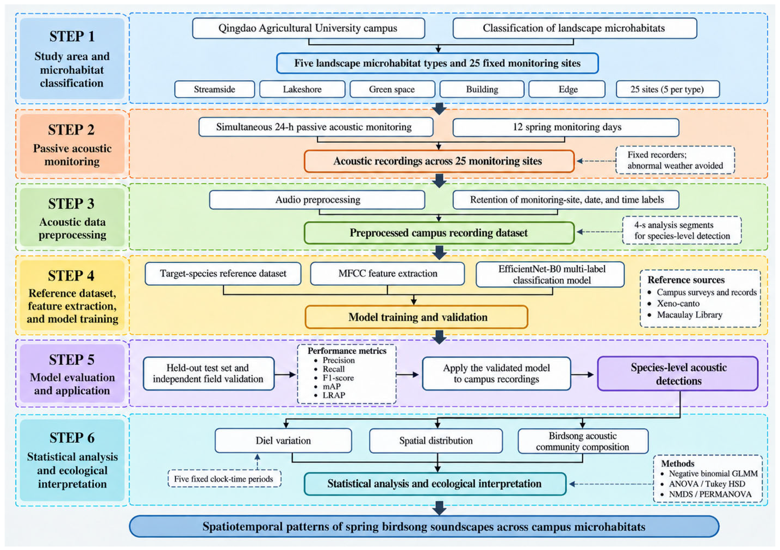
The research design consisted of six sequential steps: (1) classification of the Qingdao Agricultural University campus into five landscape microhabitat types—streamside, lakeshore, green space, building, and edge—and establishment of 25 fixed monitoring sites; (2) simultaneous 24 h passive acoustic monitoring at all sites during 12 spring monitoring days; (3) preprocessing of acoustic recordings while retaining monitoring-site, date, and time labels for subsequent analysis; (4) construction of the target-species reference dataset, extraction of Mel-frequency cepstral coefficient (MFCC) features, and training and validation of the EfficientNet-B0 multi-label classification model; (5) evaluation of model performance using the held-out test set and independent field validation, followed by application of the validated model to campus recordings to generate species-level acoustic detections; and (6) statistical analyses of diel variation, spatial distribution, and birdsong acoustic community composition. Diel variation was evaluated across five fixed clock-time periods, while spatial and community-level patterns were examined using corresponding univariate and multivariate statistical approaches (Figure 1).

2.1. Study Area and Classification of Landscape Microhabitats

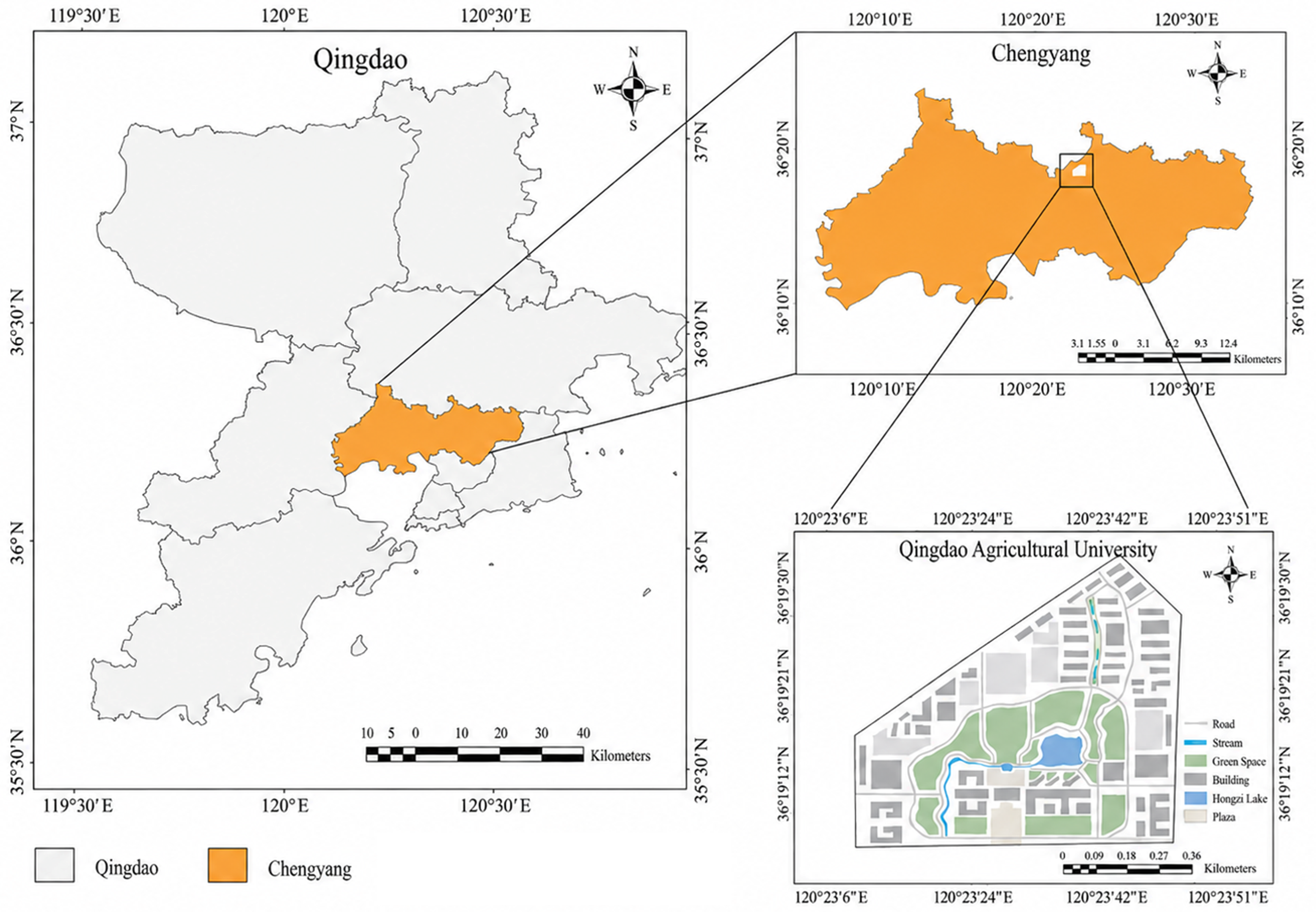
This study focused on an urban campus, with the Qingdao Agricultural University campus selected as a representative case study area. The study area is located in Chengyang District, Qingdao City, Shandong Province, China, central coordinates 36°19′14.4″ N, 120°23′30.8″ E, and has a temperate monsoon climate (Figure 2). The campus covers an area of approximately 95 hm² and consists of teaching buildings, road systems, water bodies, artificial green spaces, and semi-natural vegetation patches. Due to the limited spatial scale of the campus and the close integration of built and ecological spaces, different landscape areas differ in vegetation structure, water conditions, and levels of human disturbance, making the campus a suitable study area for investigating the relationship between micro-scale spatial characteristics and birdsong soundscape responses.

Previous studies have shown that urban avian activity is jointly influenced by vegetation structure, water availability, spatial connectivity, and human disturbance, and that different landscape units exhibit distinct patterns of avian habitat use [15]. Based on the established understanding of the relationship between spatial scales and bioacoustic responses in urban soundscape ecology [16,17], this study comprehensively considered vegetation structure, water proximity level, building disturbance level, and urban road influence level. Based on field surveys and analysis of spatial characteristics, the campus was classified into five landscape microhabitat types (

Table 1. Five landscape microhabitat types and environmental characteristics in the urban campus.

Microhabitat Type	Main Spatial Characteristics	Vegetation Structure Characteristics	Water Proximity Level	Building Disturbance Level	Urban Road Influence Level	Integrated Ecological Interpretation
Streamside	Distributed as a belt along campus streams	Continuous green corridor formed by riparian trees, shrubs, and herbaceous plants; relatively rich vertical vegetation structure	• High; adjacent to linear water bodies, providing stable water sources and moist microenvironments	• Low–moderate–high; locally influenced by surrounding buildings	• Low; far from urban roads, with weak traffic disturbance	The water–land ecotone promotes plant growth; relatively continuous vegetation provides shelter, nesting, and foraging spaces, while relatively limited human activity favors avian activity
Lakeshore	Distributed around artificial lakes and riparian buffer zones	Mainly composed of lakeshore trees and shrubs, herbaceous cover, and some aquatic plants; open toward the water surface	• High; adjacent to open water bodies with abundant aquatic resources	• Low–moderate–high; locally influenced by surrounding buildings and recreational activities	• Low; far from urban roads, with weak traffic disturbance	Water bodies and vegetation jointly form an ecological buffer zone; relatively high human activity may coexist with habitat conditions suitable for birds dependent on aquatic resources and edge environments
Green space	Located in large green–space patches within the campus	Usually composed of tree, shrub, and herbaceous layers, with high vegetation volume and good spatial continuity	• Low; far from major water bodies and dependent solely on rainfall and artificial irrigation	• Low–moderate; locally influenced by surrounding buildings	• Low; far from urban roads, with weak traffic disturbance	Multilayer vegetation increases habitat complexity; relatively limited human activity provides stable shelter and food resources for urban birds
Building	Located in open spaces around teaching buildings, dormitories, and other buildings	Mainly fragmented artificial vegetation around buildings; relatively simple planting configuration and weak continuity	• Low; far from major water bodies	• High; high building density and frequent human activity	• Low–moderate; locally influenced by urban roads	The high proportion of built space limits vegetation development; limited ecological resources and substantial noise disturbance constrain avian habitat availability
Edge	Located along the campus boundary and adjacent to urban roads	Usually composed of campus landscaping, roadside green belts, and surrounding urban vegetation; spatial continuity varies considerably	• Low; far from major water bodies	• High; jointly influenced by campus buildings and surrounding urban spaces	• High; adjacent to urban roads, with strong traffic disturbance	Strong edge effects; vegetation resources and anthropogenic disturbance jointly form a relatively complex but less stable ecological transition zone

). Streamside-type and lakeshore-type microhabitats were mainly characterized by water bodies and riparian vegetation spaces, while green space-type microhabitats were mainly characterized by continuous vegetation spaces. Building-type and edge-type microhabitats represented areas with high levels of human disturbance and campus–urban transition zones, respectively. This classification established spatial analytical units consistent with the monitoring scale of birdsong soundscapes, providing a foundation for comparing avian acoustic activity and species composition among different landscape microhabitats.

2.2. Acoustic Monitoring, Data Collection, and Preprocessing

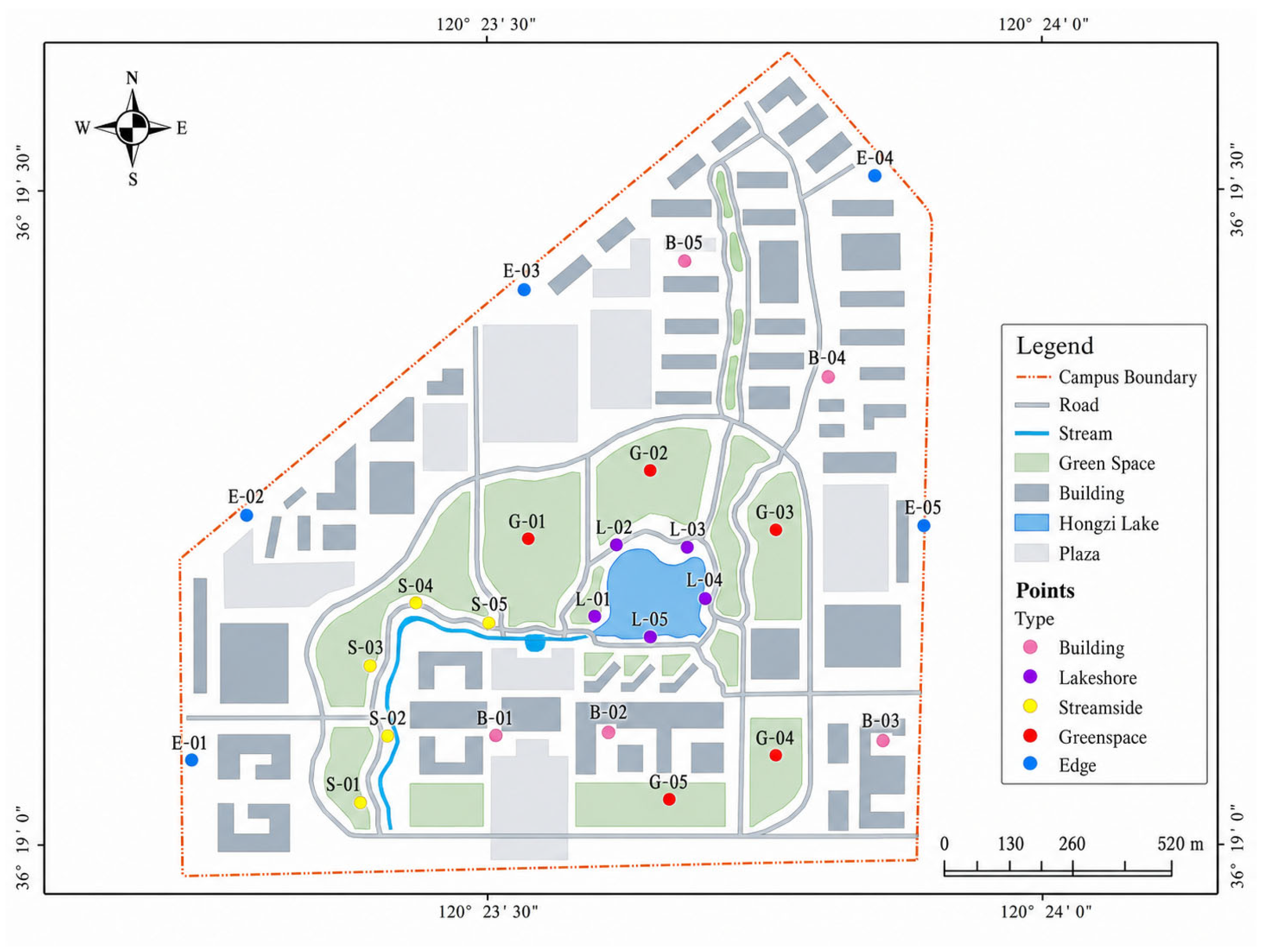
To obtain continuous dynamic information on urban campus birdsong soundscapes, passive acoustic monitoring (PAM) was used to collect spring birdsong data [18,19,20]. Acoustic monitoring was conducted on 12 days from March to May 2026 (March: 12, 13, 14, 15; April: 15, 16, 17, 18; May: 14, 15, 16, 17). Five fixed monitoring sites were established within each of the five landscape microhabitat types, resulting in 25 monitoring sites (

Table 2. Specific environmental characteristics of 25 monitoring sites across five landscape microhabitat types in the urban campus.

Microhabitat Type	Monitoring Site	Coordinates	Vegetation Structure and Cover Characteristics	Water Body Proximity	Building Interference Level	Urban Road Influence Level
Streamside	S–01	36°19′4.14″N; 120°23′38.76″E	High cover/riparian multilayer vegetation	High (<20 m)	Low (>40 m)	Low (>40 m)
	S–02	36°19′5.24″N; 120°23′21.42″E	High cover/riparian multilayer vegetation	High (<20 m)	High (<20 m)	Low (>40 m)
	S–03	36°19′8.26″N; 120°23′19.22″E	High cover/riparian multilayer vegetation	High (<20 m)	Low (>40 m)	Low (>40 m)
	S–04	36°19′11.68″N; 120°23′21.43″E	High cover/riparian multilayer vegetation	High (<20 m)	Low (>40 m)	Low (>40 m)
	S–05	36°19′11.43″N; 120°23′24.87″E	High cover/riparian multilayer vegetation	High (<20 m)	Moderate (20–40 m)	Low (>40 m)
Lakeshore	L–01	36°19′11.95″N; 120°23′32.18″E	Moderate–high cover/continuous shore–edge vegetation	High (<20 m)	Moderate (20–40 m)	Low (>40 m)
	L–02	36°19′14.68″N; 120°23′32.99″E	Moderate–high cover/continuous shore–edge vegetation	High (<20 m)	Low (>40 m)	Low (>40 m)
	L–03	36°19′14.58″N; 120°23′37.63″E	Moderate–high cover/continuous shore–edge vegetation	High (<20 m)	Low (>40 m)	Low (>40 m)
	L–04	36°19′12.25″N; 120°23′38.68″E	Moderate–high cover/continuous shore–edge vegetation	High (<20 m)	Low (>40 m)	Low (>40 m)
	L–05	36°19′10.72″N; 120°23′35.01″E	Moderate–high cover/continuous shore–edge vegetation	High (<20 m)	High (<20 m)	Low (>40 m)
Green space	G–01	36°19′15.48″N; 120°23′29.03″E	High cover/tree–shrub–herb composite green space	Low (>40 m)	Low (>40 m)	Low (>40 m)
	G–02	36°19′18.46″N; 120°23′34.71″E	High cover/tree–shrub–herb composite green space	Low (>40 m)	Low (>40 m)	Low (>40 m)
	G–03	36°19′16.78″N; 120°23′41.40″E	High cover/tree–shrub–herb composite green space	Low (>40 m)	Low (>40 m)	Low (>40 m)
	G–04	36°19′5.74″N; 120°23′41.97″E	High cover/tree–shrub–herb composite green space	Low (>40 m)	Moderate (20–40 m)	Low (>40 m)
	G–05	36°19′3.62″N; 120°23′35.52″E	High cover/tree–shrub–herb composite green space	Low (>40 m)	Moderate (20–40 m)	Low (>40 m)
Building	B–01	36°19′6.25″N; 120°23′26.30″E	Low–moderate cover/fragmented artificial vegetation structure	Low (>40 m)	High (<20 m)	Low (>40 m)
	B–02	36°19′6.91″N; 120°23′32.58″E	Low–moderate cover/fragmented artificial vegetation structure	Low (>40 m)	High (<20 m)	Low (>40 m)
	B–03	36°19′6.38″N; 120°23′47.36″E	Low–moderate cover/fragmented artificial vegetation structure	Low (>40 m)	High (<20 m)	High (<20 m)
	B–04	36°19′21.90″N; 120°23′44.63″E	Low–moderate cover/fragmented artificial vegetation structure	Low (>40 m)	High (<20 m)	Moderate (20–40 m)
	B–05	36°19′27.04″N; 120°23′38.49″E	Low–moderate cover/fragmented artificial vegetation structure	Low (>40 m)	High (<20 m)	Moderate (20–40 m)
Edge	E–01	36°19′5.43″N; 120°23′10.44″E	Moderate cover/edge–transition vegetation	Low (>40 m)	High (<20 m)	High (<20 m)
	E–02	36°19′13.98″N; 120°23′13.44″E	Moderate cover/edge–transition vegetation	Low (>40 m)	High (<20 m)	High (<20 m)
	E–03	36°19′25.30″N; 120°23′32.63″E	Moderate cover/edge–transition vegetation	Low (>40 m)	High (<20 m)	High (<20 m)
	E–04	36°19′31.42″N; 120°23′45.58″E	Moderate cover/edge–transition vegetation	Low (>40 m)	High (<20 m)	High (<20 m)
	E–05	36°19′15.30″N; 120°23′49.56″E	Moderate cover/edge–transition vegetation	Low (>40 m)	High (<20 m)	High (<20 m)

; Figure 3). All 25 monitoring sites were recorded simultaneously on the same 12 monitoring days, with continuous 24 h recording conducted at each site on each monitoring day. Thus, all sites had the same nominal temporal coverage and recording effort, allowing direct comparisons among monitoring sites and microhabitat types. Automatic recording devices (LY–S–01, Luyin, China) were used for continuous recording, with a sampling frequency of 32 kHz and a bit depth of 16 bits.

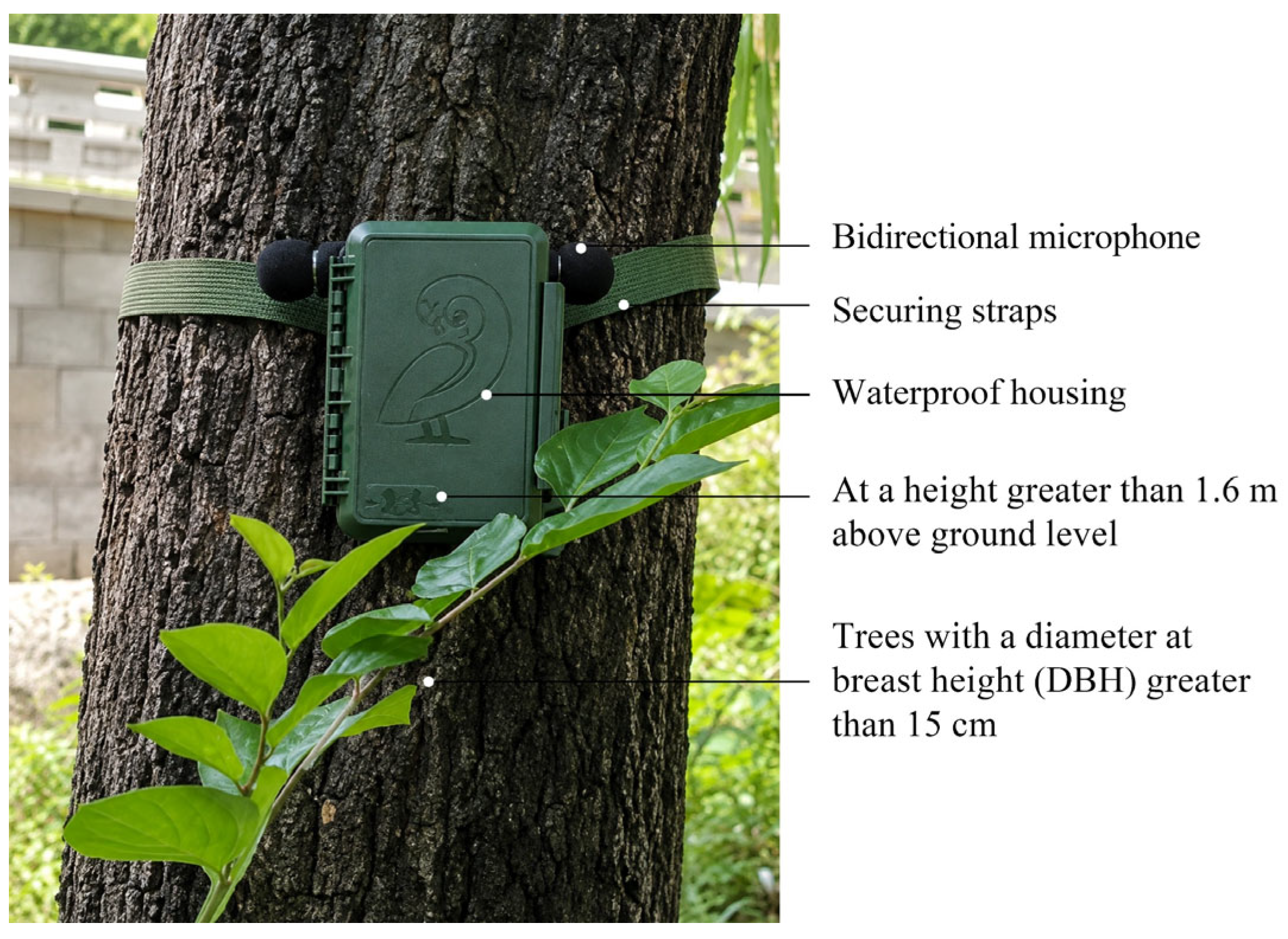
During monitoring, devices were kept fixed in place, and rainfall, strong winds, and other abnormal weather conditions were avoided to reduce the influence of abiotic environmental factors on recording quality (Figure 4). The effective recording range of each device was approximately 40 m. To reduce overlap among recording ranges, the distance between devices was maintained at more than 50 m. Recorded audio data were preprocessed following a standardized workflow, including format conversion, noise removal, removal of abnormal segments, and time-label matching, to establish a standardized acoustic dataset.

To ensure the accuracy of subsequent birdsong identification and soundscape analysis, a species-level detection was defined as one positive prediction for one target bird species within a 4 s audio segment. Because a multi-label classification strategy was used, more than one target species could be detected within the same 4 s segment; therefore, a single audio segment could contribute multiple species-level detections. All detections retained the corresponding monitoring-site, date, and time labels for subsequent aggregation and statistical analysis.

2.3. Dataset Construction

To achieve automatic bird sound identification in complex campus sound environments, an acoustic dataset for the target bird species was constructed. Target bird species were determined based on bird resource records in Qingdao, historical campus observations, and actual detections during spring monitoring. A total of 70 representative target bird species were selected as target species for identification. Therefore, the subsequent number of detected target bird species refers specifically to the number of acoustically detected species among these 70 target bird species. The complete list of the 70 target bird species, together with their migratory type, campus detection status, and species-specific classification performance, is provided in Supplementary Table S1.

Audio data for model training were mainly obtained from public bird sound databases, including Xeno–canto and the Macaulay Library. Considering differences in recording environments, signal-to-noise ratios, and acoustic characteristics among audio sources, original audio data were uniformly preprocessed, including format conversion, sampling rate standardization, selection of valid vocalization segments, and manual quality inspection, to construct standardized training samples [21,22,23,24]. The final reference dataset comprised 8400 standardized 4 s audio samples (560 min in total), with 120 samples (8.0 min) retained for each of the 70 target species. Thus, the dataset was class-balanced, with equal representation of all target species. The dataset was divided into training, validation, and held-out test sets using a class-stratified 8:1:1 split, yielding 6720, 840, and 840 samples, respectively (96, 12, and 12 samples per species). The training, validation, and test sets described above were constructed from the standardized reference recordings and were used for model development and internal performance evaluation. To independently assess the transferability of the trained model to real campus acoustic conditions, an additional field validation was subsequently conducted using manually annotated recordings collected from the study campus.

Considering the frequent occurrence of simultaneous multi-species vocalizations and background noise interference in campus environments, a multi-label classification strategy was adopted, enabling the model to identify multiple target bird species within the same audio segment. The identification results obtained from the trained model were used to calculate birdsong detection frequencies across different monitoring periods and microhabitats and to further analyze the temporal variation, spatial distribution, and species composition of birdsong soundscapes.

2.4. Acoustic Feature Extraction

To effectively characterize birdsong signals in complex campus acoustic environments, acoustic features were extracted from the preprocessed audio data. Previous studies have demonstrated that bird sounds contain rich spectral structural information, which can reflect acoustic differences among species and provide an important basis for automated identification and ecoacoustic assessment [25].

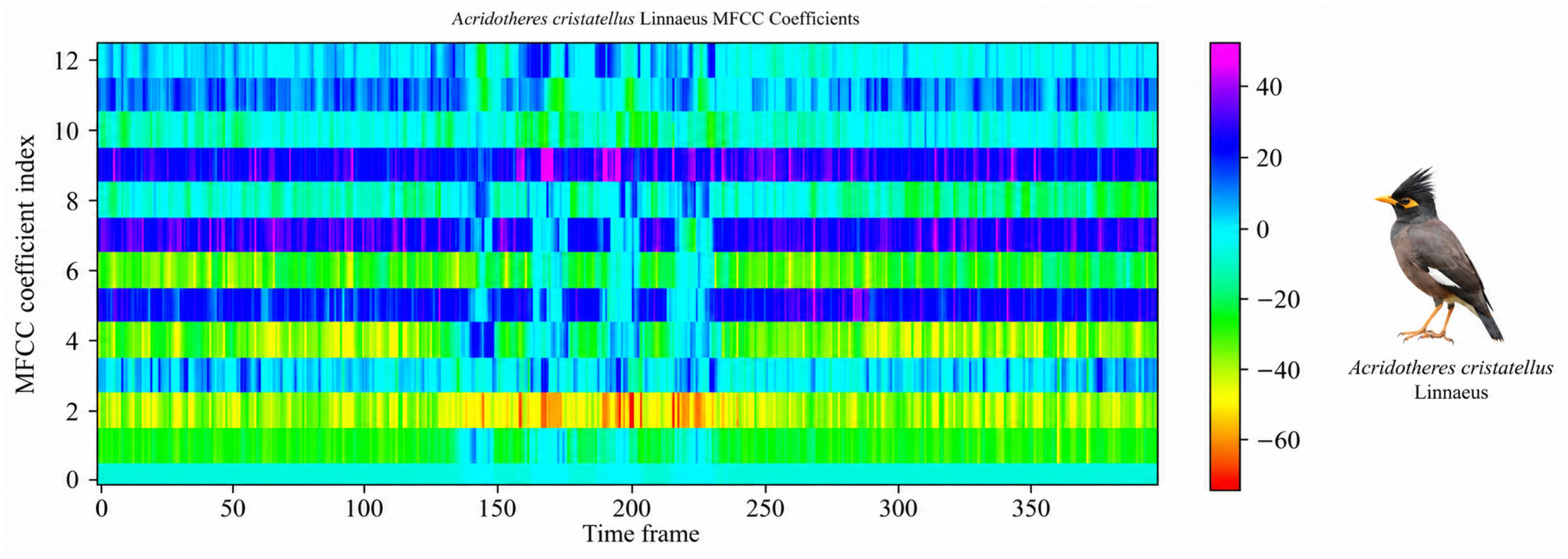
In this study, Mel-frequency cepstral coefficients (MFCC) were selected as the primary acoustic features (Figure 5). MFCC simulate human auditory perception, effectively extract spectral envelope features, and have been widely applied in bird sound identification and ecoacoustic research [26]. During processing, continuous audio signals were transformed into time–frequency representations. MFCC feature parameters were obtained through pre-emphasis, framing, windowing, fast Fourier transform (FFT), and Mel filtering. Parameter settings were as follows: sampling rate: 32 kHz; FFT window length: 2048; hop length: 512; number of Mel filters: 128; MFCC dimensionality: 13. All MFCC feature extraction was performed in Python 3.11. The extracted acoustic feature matrices were used as inputs to the deep learning model to learn acoustic differences among bird species. MFCC provide compact representations of the spectral envelope characteristics of birdsong signals, facilitating the extraction of discriminative acoustic information among bird species in complex campus sound environments and providing a data basis for subsequent birdsong identification and analysis of soundscape characteristics [27,28].

2.5. Model Construction and Training

To achieve automatic bird sound identification in complex campus acoustic environments, the EfficientNet-B0 deep learning model was used for birdsong classification. Based on a convolutional neural network architecture, this model improves classification performance in complex acoustic environments through multi-scale feature extraction and parameter optimization, making it suitable for large-scale acoustic data processing and automated identification tasks [29,30,31]. The model consists mainly of an initial convolutional layer, multiple Mobile Inverted Bottleneck Convolution (MBConv) modules, and a classification layer (Figure 6). The network structure parameters of each stage of EfficientNet-B0 are shown in

Table 3. Stage-wise network architecture and feature extraction parameters of EfficientNet-B0.

Stage i	Operator ${\widehat{\mathit{F}}}_{\mathit{i}}$	Resolution ${\widehat{\mathit{H}}}_{\mathit{i}}\times {\widehat{\mathit{W}}}_{\mathit{i}}$	#Channels ${\widehat{\mathit{C}}}_{\mathit{i}}$	#Layers ${\widehat{\mathit{L}}}_{\mathit{i}}$
1	Conv3 × 3	224 × 224	32	1
2	MBConv1, k3 × 3	112 × 112	16	1
3	MBConv6, k3 × 3	112 × 112	24	2
4	MBConv6, k5 × 5	56 × 56	40	2
5	MBConv6, k3 × 3	28 × 28	80	3
6	MBConv6, k5 × 5	14 × 14	112	3
7	MBConv6, k5 × 5	14 × 14	192	4
8	MBConv6, k3 × 3	7 × 7	320	1
9	Conv1 × 1 & Pooling & FC	7 × 7	1280	1

.

Considering the characteristics of simultaneous multi-species vocalizations in campus environments, a multi-label classification strategy was adopted, enabling the model to identify multiple target bird species within the same audio segment. The output layer used the Sigmoid activation function to independently calculate occurrence probabilities for each bird species category. Binary Cross Entropy (BCE) was used as the loss function during training, and its calculation is given as follows:

$$L=-{\displaystyle \frac{1}{N}}\sum _{i=1}^N\left[y_i\log \left(p_i\right)+\left(1 |-|y_i\right)\log \left(1 |-|p_i\right)\right]$$

(1)

where $N$ denotes the number of samples, $y_i$ denotes the true label value, and $p_i$ denotes the model-predicted probability. The BCE loss function effectively measures the difference between the predicted probabilities and the true species labels. A transfer learning strategy was adopted during model training. The EfficientNet-B0 backbone was initialized with pretrained weights from BirdCLEF2023 and subsequently fine-tuned using the birdsong training set. Model optimization was performed using the AdamW optimizer with an initial learning rate of 1 × 10⁻⁴, a batch size of 32, and a weight decay of 1 × 10⁻⁴. The model was trained for a maximum of 50 epochs, with early stopping applied when the validation loss failed to improve for eight consecutive epochs. No additional data augmentation was applied beyond the standardized preprocessing procedures described in Section 2.3.

2.6. Model Performance Evaluation

To evaluate the classification performance of the EfficientNet-B0 model on the held–out test set, micro-averaged Precision, Recall, and F1 score were used as the primary overall evaluation metrics. Overall Precision, Recall, and F1 score were calculated by pooling predictions across all target species, whereas species-specific Precision, Recall, and F1 score were calculated separately for each of the 70 target species. Precision measures the accuracy of the bird species predicted by the model, Recall evaluates the model’s ability to identify the true bird species, and F1 score reflects the balance between model accuracy and identification completeness.

Considering the multi-label classification characteristics of campus recordings involving simultaneous vocalizations from multiple bird species, mean Average Precision (mAP) and Label Ranking Average Precision (LRAP) were further used to evaluate the model’s ability to identify birdsong signals from multiple bird species. Among these metrics, mAP measures the overall identification precision of the model across different bird species categories. Its calculation is given as follows:

$$mAP={\displaystyle \frac{1}{C}}\sum _{c=1}^{C}A{P}_c$$

(2)

where C denotes the total number of target bird species (70 in this study), and $A{P}_c$ denotes the average precision for the Cth bird species. An mAP value closer to 1 indicates stronger identification performance of the model across different bird species categories.

LRAP was used to evaluate the consistency between the ranking of model output probabilities and the set of true labels. Its calculation is given as follows:

$$LRAP={\displaystyle \frac{1}{N}}\sum _{i=1}^N{\displaystyle \frac{1}{\left|Y_i\right|}}\sum _{y\in Y_i}{\displaystyle \frac{\left|\{y^{\prime }\in Y_i:\mathrm{ran}{k}_i\left(y^{\prime }\right)\le ran{k}_i\left(y\right)\}\right|}{ran{k}_i\left(y\right)}}$$

(3)

where $N$ denotes the total number of test samples; $Y_i$ denotes the set of true bird species labels corresponding to the ith sample; $\left|Y_i\right|$ denotes the number of true bird species in that sample; and $ran{k}_i\left(y\right)$ denotes the ranking position of the probability assigned to bird species y in the model predictions. An LRAP value closer to 1 indicates that the model can more accurately distinguish the probability ranking relationships among multiple simultaneously occurring bird species.

To further evaluate the applicability of the trained model under real campus acoustic conditions, an independent field validation was conducted using recordings collected during the campus monitoring campaign. A total of 1250 non-overlapping 4 s audio segments were randomly selected from the original monitoring recordings using a stratified sampling procedure, with samples distributed across all five landscape microhabitat types, five fixed clock-time periods, 25 monitoring sites, and 12 monitoring days to reduce potential spatial and temporal sampling bias. The field-validation recordings were completely independent of the reference recordings used for model development and were not included in model training, validation, parameter tuning, internal testing, or threshold selection. Two researchers familiar with local bird vocalizations independently reviewed each selected audio segment and annotated the presence or absence of the target bird species. Disagreements between the two annotators were resolved through joint re-examination and consensus, and the resulting annotations were used as reference labels. Model output probabilities were converted into binary species detections using a fixed probability threshold of 0.50. The same threshold was applied consistently, without re-optimization, to the held-out test set, the independent field-validation dataset, and the complete campus monitoring dataset. Precision, Recall, F1 score, and mean Average Precision (mAP) were subsequently calculated by comparing model predictions with the manually annotated reference labels to assess the transfer performance of the trained model under real campus recording conditions.

2.7. Statistical Analysis

Based on the birdsong identification results, this study analyzed the birdsong soundscape characteristics of different landscape microhabitat types from three aspects: diel variation, spatial distribution, and species composition. All statistical analyses were conducted using R 4.3 software, with the significance level set at α = 0.05.

For diel analysis, the 24 h continuous monitoring data were divided into five standardized fixed clock-time periods: Late night (00:00–04:00), Early morning (04:00–06:00), Daytime (06:00–17:00), Evening (17:00–19:00), and Night (19:00–24:00). These categories were used to maintain a consistent temporal classification across all monitoring dates and sites; therefore, “Early morning” and “Evening” refer to fixed clock-time periods rather than the exact astronomical sunrise and sunset times on individual monitoring dates. For diel variation analysis, the site × monitoring date × fixed clock-time period was used as the basic analytical unit, and the total number of species-level birdsong detections was calculated for each analytical unit. A negative binomial generalized linear mixed-effects model (GLMM) was used to account for the non-independence of repeated observations from the same monitoring sites and to accommodate the count nature of the response variable. Landscape microhabitat type, fixed clock-time period, and their interaction were included as fixed effects, whereas monitoring site and monitoring date were included as crossed random intercepts. To account for differences in recording duration among the five fixed clock-time periods, the logarithm of recording duration (h) was included as an offset term. Pairwise comparisons were subsequently performed using estimated marginal means with Tukey adjustment when significant fixed effects were detected. For descriptive summaries of diel variation, species-level detection rates were calculated for each site × monitoring date × fixed clock-time period as the number of species-level detections divided by the corresponding recording duration (h). These unit-level rates were then summarized within each microhabitat × period combination using the mean and its 95% confidence interval. The resulting descriptive means, expressed as detections per site–hour, and their 95% confidence intervals were used to visualize overall diel patterns in Figure 7A and were not treated as independent observations in the GLMM.

For each monitoring site, birdsong detection count was calculated as the cumulative number of species-level detections obtained across the 12 monitoring days; because all sites were monitored simultaneously for the same duration, these cumulative counts were directly comparable among sites. The individual monitoring site was used as the independent analytical unit for the spatial analysis, resulting in 25 site-level observations (n = 5 sites per microhabitat type). One-way analysis of variance (one-way ANOVA) was conducted to compare differences in birdsong detection count and the number of detected target bird species among the five landscape microhabitat types. Effect size was quantified using eta-squared (η²), and 95% confidence intervals for η² were estimated based on the noncentral F distribution. Descriptive statistical analysis was also performed to characterize variation patterns among different spatial units. In addition, Spearman correlation analysis was used to evaluate the consistency between avian acoustic activity levels and species detection characteristics.

For species composition analysis, a species composition matrix was constructed based on birdsong detection frequency of target bird species across different landscape microhabitats and fixed clock-time periods. Non-metric multidimensional scaling (NMDS) based on Bray–Curtis dissimilarity was used to visualize differences in birdsong acoustic community composition among groups. Permutational multivariate analysis of variance (PERMANOVA) was applied to test the effects of landscape microhabitat type, fixed clock-time period, and their interaction on community composition, with R² reported as the corresponding effect size. Homogeneity of multivariate dispersion was additionally assessed using PERMDISP for microhabitat types and fixed clock-time periods. Because significant differences in dispersion can contribute to PERMANOVA significance, PERMANOVA results were interpreted together with the corresponding PERMDISP results.

For species-level analyses, the same site × monitoring date × fixed clock-time period analytical structure and negative binomial GLMM framework described above were applied separately to each of the 65 detected target bird species. Landscape microhabitat type, fixed clock-time period, and their interaction were included as fixed effects, with monitoring site and monitoring date as crossed random intercepts and recording duration included as an offset. To account for multiple testing across species, p values for each effect were adjusted using the Benjamini–Hochberg false discovery rate (FDR) procedure, with an adjusted p < 0.05 considered significant.

3. Results

3.1. Model Performance and Field Validation

The EfficientNet-B0 model showed good classification performance on the held-out test set (

Table 4. Classification performance of the EfficientNet-B0 birdsong identification model on the held-out test set.

Model	Total Number of Reference Samples	Total Sample Duration (min)	Micro-Precision	Micro-Recall	Micro-F1 Score	mAP	LRAP
EfficientNet-B0 birdsong identification model	8400	560	0.850	0.830	0.840	0.925	0.936

). The training and validation losses gradually decreased and stabilized during training, indicating stable model convergence. Species-specific Precision, Recall, and F1-score for all 70 target bird species on the held-out test set are reported in Supplementary Table S1.

The independent field validation showed that the model retained generally good classification performance when applied to complex campus recordings, achieving a micro-Precision of 0.830, micro-Recall of 0.800, micro-F1 score of 0.815, and mAP of 0.880. Species-specific field-validation results, including the number of manually confirmed positive clips and the corresponding Precision, Recall, and F1-score for each target species represented in the validation dataset, are provided in Supplementary Table S1. Although these values were slightly lower than those obtained from the held-out test set, the field-validation results supported the applicability of the trained model for characterizing relative patterns of avian acoustic activity across the campus. Nevertheless, because automated acoustic identification cannot completely eliminate false-positive and false-negative detections, the subsequent results are interpreted as model-assisted patterns of acoustic detections rather than direct estimates of bird abundance or population size.

3.2. Diel Variation Characteristics of Birdsong Soundscapes Among Different Landscape Microhabitat Types

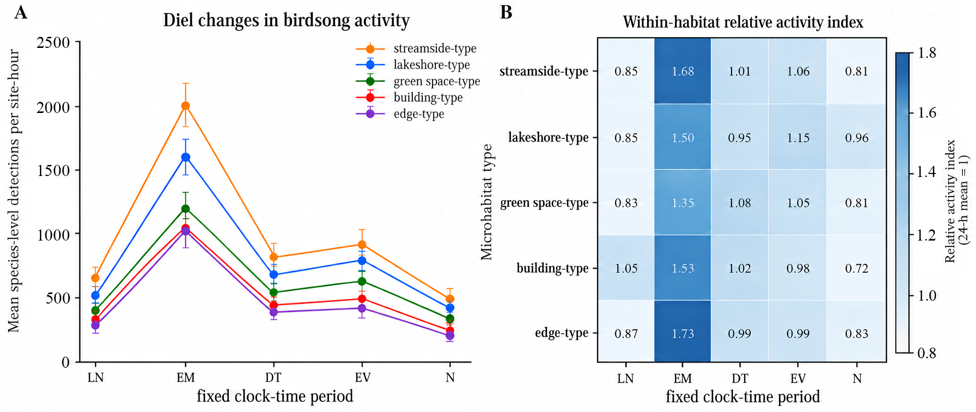
Birdsong soundscapes across the five landscape microhabitat types exhibited clear diel rhythms (Figure 7). The negative binomial GLMM showed significant effects of landscape microhabitat type (χ²₄ = 118.72, p < 0.001) and fixed clock-time period (χ²₄ = 84.36, p < 0.001) on birdsong detection rates, whereas their interaction was not significant (χ²₁₆ = 24.60, p = 0.077). Thus, after accounting for repeated observations from the same monitoring sites, variation among monitoring dates, and differences in recording duration among periods, the five landscape microhabitat types generally retained similar diel variation patterns while differing in their overall levels of avian acoustic activity.

Figure 7A shows that avian acoustic activity remained relatively low during the Late night period. During Early morning, avian acoustic activity increased rapidly and reached the main peak of the day. The mean species-level detection rates were 2004.5, 1616.3, 1192.8, 1048.2, and 1028.2 detections per site-hour for streamside-type, lakeshore-type, green space-type, building-type, and edge-type microhabitats, respectively. Based on the estimated marginal means of the fixed clock-time period effect, birdsong detection rates during Early morning were significantly higher than those during all other fixed clock-time periods (Tukey-adjusted pairwise comparisons, all p < 0.05). During Evening, the mean species-level detection rates in streamside-type and lakeshore-type microhabitats increased to 1262.1 and 1241.4 detections per site-hour, respectively, forming a clear secondary evening peak, whereas green space-type microhabitats showed relatively gradual changes. Building-type and edge-type microhabitats did not show obvious increases. During Night, avian acoustic activity decreased again, with particularly low values observed in building-type and edge-type microhabitats.

Relative activity indices were calculated by normalizing the 24 h mean hourly pooled birdsong detection count of each microhabitat type to 1. Figure 7B shows that the relative activity indices of all five microhabitat types were substantially higher than their respective 24 h mean levels during Early morning. The highest index was observed in edge-type microhabitats (1.73), followed by streamside-type microhabitats (1.68), indicating that although edge-type microhabitats had lower absolute avian acoustic activity levels, they showed the greatest increase relative to their own background activity during Early morning. During Evening, the relative indices of streamside-type, lakeshore-type, and green space-type microhabitats were approximately 1.06, 1.15, and 1.05, respectively, whereas those of building-type and edge-type microhabitats were close to 1. During Night, avian acoustic activity in all microhabitat types decreased to relatively low levels. Overall, the five landscape microhabitat types shared a common diel pattern characterized by low activity during Late night, a rapid increase to the main peak during Early morning, a decline to moderate levels during Daytime, secondary evening peaks in some microhabitats, and a further decrease during Night.

3.3. Spatial Distribution Characteristics of Birdsong Soundscapes Among Different Landscape Microhabitat Types

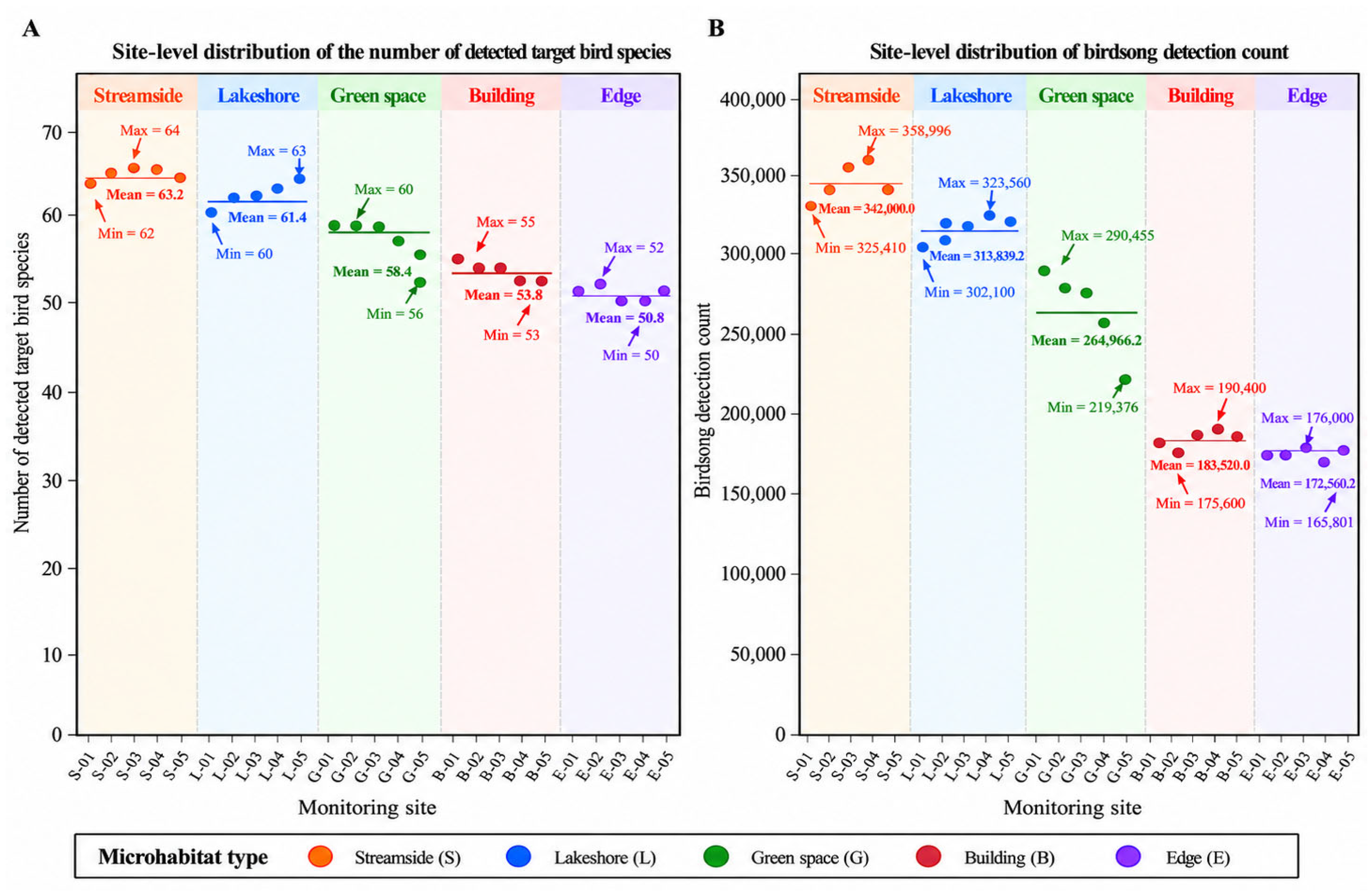
The number of detected target bird species and birdsong detection count across the 25 monitoring sites showed clear spatial differentiation (Figure 8). The number of detected target bird species differed significantly among the five landscape microhabitat types (F₄,₂₀ = 92. 96, p < 0.001, η² = 0.949,95% CI [0.869, 0.963]). Streamside-type and lakeshore-type microhabitats had the highest numbers of detected target bird species (63.2 ± 0. 84 and 61.4 ± 0.89 species, respectively), followed by green space-type microhabitats (58.4 ± 1. 82 species), whereas building-type and edge-type microhabitats showed lower values (53.8 ± 1.30 and 50.8 ± 0.84 species, respectively). No significant difference was observed between streamside-type and lakeshore-type microhabitats (p = 0.164), whereas all other pairwise comparisons were significant. Birdsong detection count also differed significantly among the five landscape microhabitat types (F₄,₂₀ = 106.09, p < 0.001, η² = 0.955, 95% CI [0.885, 0. 967]), ranking as follows: streamside-type > lakeshore-type > green space-type > building-type > edge-type. Only building-type and edge-type microhabitats showed no significant difference (p = 0.118). At the monitoring-site scale, S–03 and S–04 each detected 64 target bird species, with S–04 showing the highest cumulative birdsong detection count over the 12 monitoring days (358,996 detections). E–03 and E–04 each detected 50 target bird species, with E–04 showing the lowest cumulative detection count (165,801 detections). Lakeshore-type microhabitats exhibited relatively small variation among sites, whereas green space-type microhabitats showed the greatest internal heterogeneity. From G–01 to G–05, the number of detected target bird species decreased from 60 to 56, while birdsong detection count decreased from 290,455 to 219,376 detections. The coefficient of variation of birdsong detection count was highest in green space-type microhabitats (10.58%). Edge-type microhabitats showed the most concentrated spatial distribution, with a coefficient of variation of only 2.36%. A very strong positive correlation was observed between the number of detected target bird species and birdsong detection count across the 25 monitoring sites (Spearman ρ = 0.996, p < 0.001), indicating a highly consistent spatial variation pattern between the two indicators.

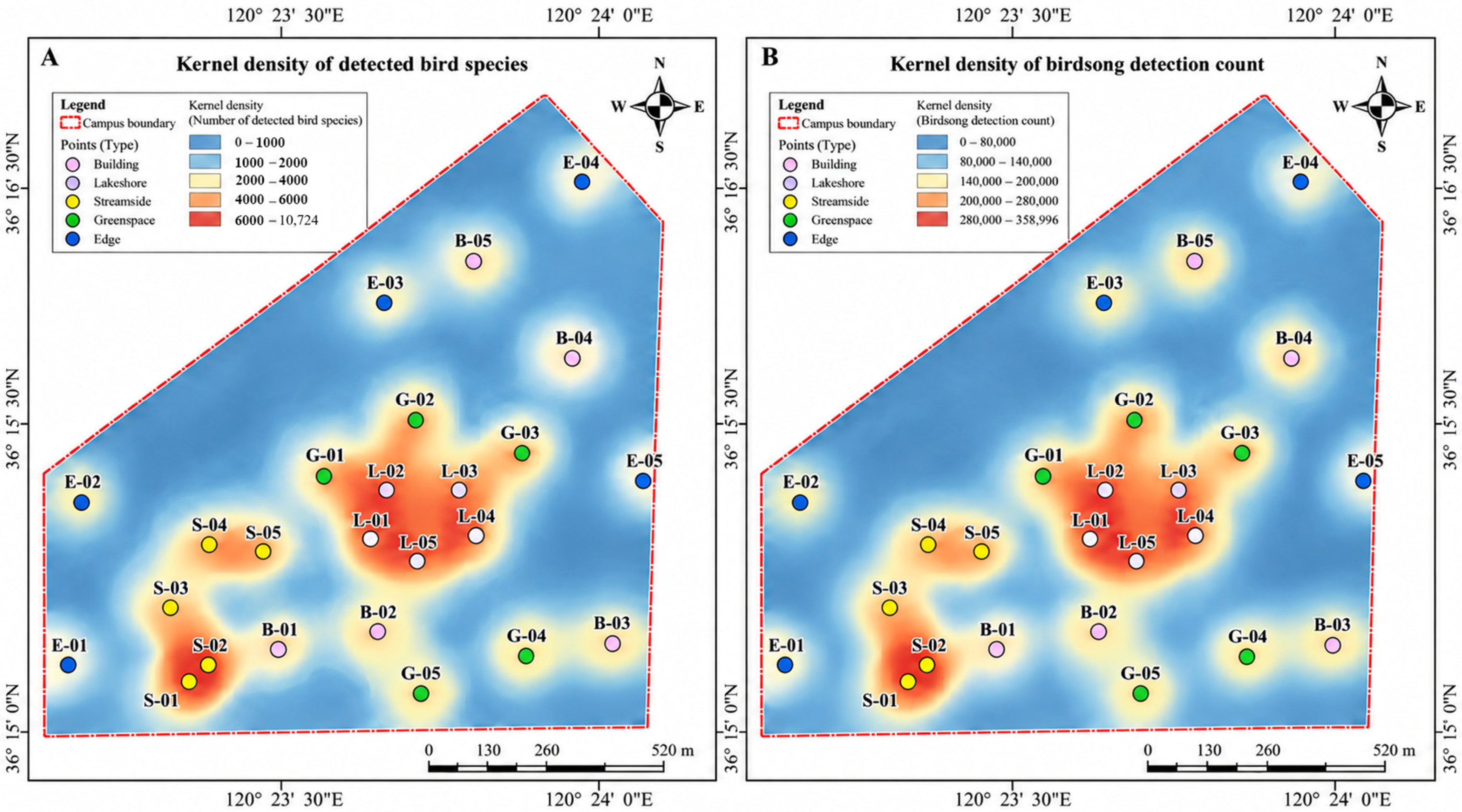
Overall, a decreasing spatial gradient was observed from riparian habitats to green spaces, buildings, and campus edge areas (Figure 9). Notably, a higher cumulative birdsong detection count may increase the probability of detecting target bird species; therefore, the correlation between the two indicators primarily reflects the consistency of their spatial variation patterns.

3.4. Characteristics of Birdsong Acoustic Community Composition Among Different Landscape Microhabitat Types

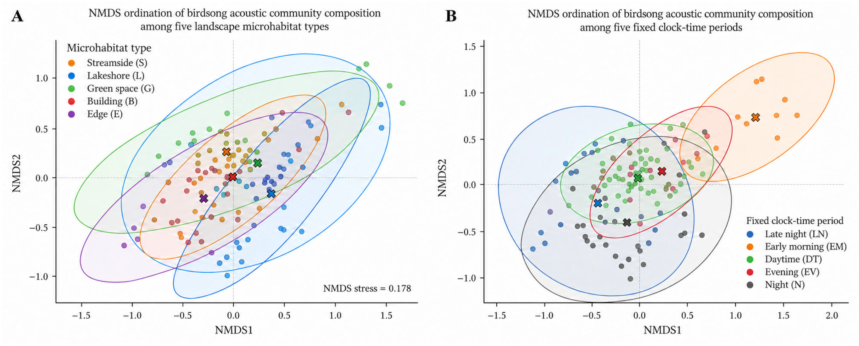
Among the 70 target bird species, 65 species were detected during the monitoring period, whereas five species were not detected. The complete species inventory, including the identities of the 65 detected and five undetected target species, is provided in Supplementary Table S1. PERMANOVA based on Bray–Curtis distance showed that landscape microhabitat type (pseudo-F₄,₉₅ = 16. 64, R² = 0. 223, p < 0.001), fixed clock-time period (pseudo–F₄,₉₅ = 22. 81, R² = 0. 306, p < 0.001), and the interaction between landscape microhabitat type and fixed clock-time period (pseudo-F₁₆,₉₅ = 2.85, R² = 0.153, p < 0.001) all significantly influenced birdsong acoustic community composition, collectively explaining 68.2% of the variation in community composition. NMDS ordination yielded a stress value of 0.178, indicating a moderate but acceptable two-dimensional representation of the multivariate dissimilarity structure. Accordingly, the ordination was used primarily to interpret broad patterns of group separation rather than fine–scale distances among individual samples (Figure 10).

Pairwise comparisons among landscape microhabitat types were all significant (Holm-adjusted p ≤ 0.0022), and all pairwise comparisons among fixed clock-time periods were also significant. Early morning showed pronounced differentiation from Late night and Night, whereas Daytime and Evening were the most similar (adjusted p = 0.035).

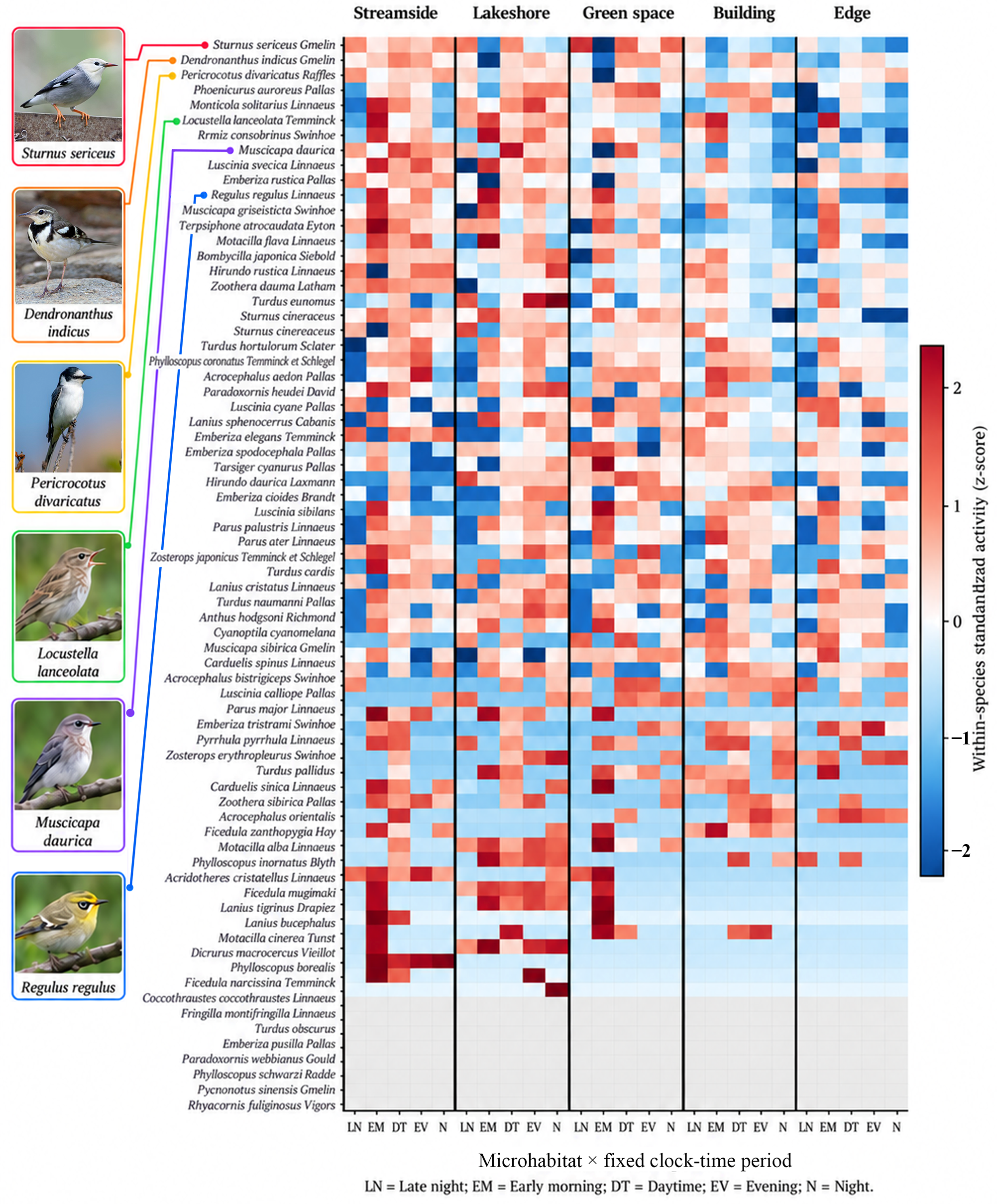
Species-level analysis further showed that, after Benjamini–Hochberg FDR correction, 46 of the 65 detected bird species exhibited significant microhabitat effects, 55 species exhibited significant fixed clock-time period effects, and 31 species showed significant microhabitat × fixed clock-time period interactions. These results indicate that the birdsong soundscape activity of most species exhibited pronounced spatial and temporal differences, and that the diel activity patterns of some species varied among microhabitats. Sturnus sericeus had the highest overall detection frequency and showed relatively high activity in green space-type microhabitats. Dendronanthus indicus and Pericrocotus divaricatus were generally associated with streamside-type microhabitats, whereas Locustella lanceolata and Regulus regulus were relatively active in lakeshore-type microhabitats and during Early morning. Muscicapa dauurica was particularly prominent in lakeshore-type microhabitats during Daytime. Figure 11 further showed distinct combinations of birdsong soundscape activity among different bird species across the five landscape microhabitat types and five fixed clock-time periods. PERMDISP showed no significant difference in multivariate dispersion among microhabitat types (p = 0.453), supporting the interpretation that the PERMANOVA differences among microhabitats primarily reflected differences in community composition rather than unequal within-group dispersion. In contrast, multivariate dispersion differed significantly among fixed clock-time periods (p = 0.001). Therefore, the significant PERMANOVA effect of fixed clock-time period may reflect both differences in group centroids and differences in within-period dispersion and should not be interpreted solely as a shift in community centroid. Overall, the multivariate analyses indicated clear spatiotemporal structuring of birdsong acoustic community composition, although the temporal differences were interpreted with appropriate caution because of the significant PERMDISP result.

4. Discussion

4.1. Diel Rhythms of Spring Birdsong Soundscapes in Urban Campuses and Their Implications for Dynamic Assessment

Urban campuses are complex landscapes comprising buildings, roads, water bodies, and vegetation patches. Their birdsong soundscapes are jointly influenced by avian activity rhythms, spatial environmental conditions, and human activity cycles, resulting in dynamic variation. This study found that birdsong soundscapes across the five landscape microhabitat types exhibited relatively consistent diel variation patterns, characterized by low activity during Late night, a rapid rise to peak activity during Early morning, continued fluctuations during Daytime, and gradual decreases during Night. The pronounced diel pattern observed in this study is consistent with previous reports of periodic variation in avian acoustic activity [32], showing that similar temporal organization can also be detected across multiple fine-scale landscape microhabitats within a single urban campus.

Spring is an active period for breeding and migration activities of birds in temperate regions, and avian vocalization is often concentrated during the early morning because of territorial competition, individual communication, and reproductive activities [33]. In this study, all landscape microhabitat types showed a marked increase in avian acoustic activity during the fixed Early morning period, indicating a pronounced morning peak in birdsong activity. Meanwhile, the absolute levels of avian acoustic activity during the morning peak differed among landscape microhabitat types, with streamside-type, lakeshore-type, and green space-type microhabitats showing higher birdsong detection levels, whereas building-type and edge-type microhabitats showed relatively lower levels. These differences may be associated with spatial environmental factors such as vegetation structure, water conditions, and human disturbance levels.

Beyond natural behavioral rhythms, human activity cycles also shape urban biophonic soundscapes. Previous studies have suggested that anthropogenic noise may reduce birdsong signal detectability through frequency masking and temporal interference, and may affect soundscape structure in urban environments [34]. In this study, different landscape microhabitat types continued to exhibit a certain degree of fluctuation in birdsong activity during the Daytime period, potentially reflecting a dynamic association between campus space-use rhythms and natural acoustic activity. However, because traffic flow, human activity intensity, and environmental noise indicators were not simultaneously collected, the specific mechanisms by which human disturbance affects birdsong variation could not be further analyzed.

The similarities and differences in temporal variation patterns among different landscape microhabitat types reflect the influence of campus spatial structure on birdsong soundscape characteristics. Previous studies have indicated that small-scale spatial structures can influence the propagation of biological sounds, and that different combinations of green spaces, water bodies, and buildings can form distinct soundscape units [35]. Therefore, the temporal rhythms of spring birdsong soundscapes not only reflect natural cycles of avian activity but also provide a basis for assessing ecoacoustic responses across different spatial units within the campus. Future campus landscape optimization could incorporate the temporal characteristics of birdsong soundscapes, strengthen the protection and improvement of riparian spaces, continuous green spaces, and low-disturbance areas, and use continuous acoustic monitoring to evaluate the effects of spatial adjustments on the campus ecoacoustic environment.

4.2. Differences Among Landscape Microhabitats in Urban Campuses and Spatial Differentiation of Birdsong Soundscapes

Although urban campuses are limited in spatial scale, different spatial units vary in water availability, vegetation structure, building disturbance, and openness, forming landscape microhabitat types with distinct environmental characteristics. Based on birdsong acoustic monitoring across the five campus landscape microhabitats, this study found spatial differentiation in avian acoustic activity levels and species composition among different landscape microhabitats. Overall, streamside-type, lakeshore-type, and green space-type microhabitats showed higher levels, whereas building-type and edge-type microhabitats showed relatively lower levels. These results indicate a correspondence between micro-scale landscape spatial structure and birdsong soundscape characteristics, suggesting that landscape microhabitat types can serve as important spatial units for assessing differences in campus ecoacoustic environments.

Consistent with previous studies showing that urban bird distributions are associated with green-space heterogeneity, structural complexity, vegetation composition, and surrounding disturbance [36], the present study found higher levels of avian acoustic activity and higher numbers of detected target bird species in streamside-type and lakeshore-type microhabitats. This correspondence indicates that the fine-scale ecoacoustic differences observed within the campus are broadly aligned with existing evidence on habitat heterogeneity in urban bird communities. The continuous spatial interfaces formed by water bodies and vegetation provide diverse environmental conditions for avian activity and influence the propagation and detection of birdsong signals. Notably this study evaluated avian acoustic activity levels rather than directly reflecting bird abundance or population size. Therefore, differences among habitats should be interpreted as differences in acoustic responses.

Green space-type microhabitats showed advantages in avian acoustic activity and species composition, reflecting the supporting role of continuous vegetation spaces in campus birdsong diversity. Compared with single-layer vegetation, green spaces with multilayered vegetation structures comprising trees, shrubs, and herbaceous plants can provide more diverse spatial resources. In contrast, the lower levels of avian acoustic activity in building-type and edge-type microhabitats may be associated with disturbance environments generated by building interfaces, road traffic, and human activities. Previous studies have shown that changes in the acoustic environment caused by human activities may affect the propagation of bird sounds and acoustic communication processes, thereby altering birdsong patterns in urban environments [37]. Since vegetation structure and anthropogenic disturbance factors were not independently quantified in this study, differences among microhabitats should be interpreted as associations between integrated landscape characteristics and birdsong soundscape responses rather than as causal effects of individual factors.

Species composition analysis showed that although different landscape microhabitats shared some dominant bird species, they still exhibited a certain degree of spatial differentiation, indicating that campus spaces differed not only in avian acoustic activity levels but also in acoustic community composition. The spatial differentiation in birdsong acoustic community composition observed in this study is consistent with previous evidence that urban habitat heterogeneity is associated with greater complexity in bird community composition and that different types of green spaces can jointly contribute to urban biodiversity [38]. Our findings add a fine-scale ecoacoustic perspective by showing that such differentiation can also be detected among landscape microhabitats within a single urban campus. Therefore, campus landscape planning should not focus solely on increasing green space area, but should also emphasize the compositional relationships among water bodies, vegetation, building spaces, and edge spaces. Establishing a continuous and diverse network of microhabitats can thereby improve the quality of the campus ecoacoustic environment.

Overall, this study revealed an association between landscape microhabitat variation and spatial differentiation in birdsong soundscapes within the study campus. Passive acoustic monitoring can provide a complementary perspective for identifying acoustic responses of different landscape units at fine spatial scales. In campus renewal, birdsong soundscape monitoring may therefore be considered as one source of supporting evidence for the context-specific management of riparian zones, vegetation patches, and buffer areas around buildings, rather than as a stand-alone basis for planning decisions.

4.3. Implications of Birdsong Soundscape Assessment for Bird-Friendly Campus Landscape Planning

Urban campuses have limited spatial capacity and multifunctional uses. Improving ecological service capacity while meeting educational, residential, and transportation needs is an important aspect of campus landscape optimization. Based on continuous passive acoustic monitoring and deep learning-based birdsong identification, this study comprehensively evaluated the diel rhythms, spatial distribution, and species composition of birdsong soundscapes across different landscape microhabitats, providing an ecoacoustic perspective for bird-friendly campus landscape planning. Compared with approaches based solely on vegetation area, green space proportion, or manual surveys, birdsong soundscapes can reflect the dynamic variation of avian activity across temporal and spatial scales, providing a continuous and non-invasive monitoring approach for urban campus ecological assessment [39].

The results showed clear differences in birdsong soundscapes among landscape microhabitats. Streamside-type, lakeshore-type, and green space-type microhabitats showed higher levels of avian acoustic activity and higher numbers of detected target bird species, whereas building-type and edge-type microhabitats showed lower levels. These spatial differences suggest that, within the study campus, landscape optimization may consider not only the quantity of green spaces but also the compositional relationships and ecological connectivity among water bodies, vegetation, and built environments. Previous studies have indicated that structural optimization and ecological design of urban green spaces can enhance regional biodiversity and improve connections between people and the natural environment [40,41]. Considering the birdsong soundscape responses observed at the study campus, differentiated management strategies may be considered as context-specific planning implications: streamside-type and lakeshore-type microhabitats could prioritize maintaining the continuity of riparian vegetation and water–land interfaces while reducing fragmentation of existing riparian ecological zones; green space-type microhabitats could strengthen multilayered vegetation structures comprising trees, shrubs, and herbaceous plants, as well as patch connectivity; and building-type and edge-type microhabitats could enhance ecological transitions between built and natural spaces and improve connectivity among microhabitats through vegetation buffers, small-scale ecological nodes, and corridor connections.

Different landscape microhabitats exhibited not only differences in birdsong activity intensity but also clear differentiation in birdsong acoustic community composition, indicating functional differences in avian habitat use and acoustic responses among different landscape spaces. Therefore, the findings from this case study suggest that bird-friendly campus landscape design may benefit from moving beyond an exclusive emphasis on “spatial quantity optimization” toward greater consideration of “spatial function matching” informed by birdsong soundscape responses. In planning, campus green spaces should not be treated as homogeneous spaces with similar structures and functions. Instead, the spatial and ecological heterogeneity of different microhabitat types should be maintained through the combined configuration of riparian habitats, multilayered green spaces, transitional edge spaces, and distributed ecological nodes. At the same time, differentiated designs can be implemented according to the avian acoustic responses of different landscape microhabitats, enabling different types of spaces to provide complementary conditions for foraging, shelter, resting, and acoustic communication, thereby enhancing the overall capacity of the campus landscape network to support the activity requirements of different bird species. This planning approach further transforms birdsong soundscape assessment from simply describing the “level of birdsong activity” into a planning basis for identifying differences in the ecological functions of different landscape spaces.

It should be noted that the birdsong detection results in this study mainly reflect avian acoustic activity levels and do not directly correspond to bird abundance or overall community size. In addition, because the study was conducted at a single urban campus during one spring season, the observed spatiotemporal patterns and associated planning implications should be regarded as site- and season-specific rather than as universally representative of urban campuses. Their transferability to other campuses, climatic regions, and seasons requires further validation through multi-campus and multi-season monitoring. Although the independent validation using manually annotated campus recordings supported the field applicability of the automated recognizer, residual classification errors may still occur, particularly in recordings containing weak signals, substantial background noise, or overlapping vocalizations of acoustically similar species. In addition, vegetation structure, environmental noise, and human activity intensity were not quantified simultaneously in this study. Therefore, in practical planning applications, birdsong soundscape monitoring should be integrated with vegetation surveys, manual bird surveys, and environmental acoustic measurements to establish a more comprehensive campus ecological assessment system. Overall, passive acoustic monitoring combined with deep learning-based identification can provide continuous information on acoustic responses across different landscape microhabitats and may serve as a complementary source of evidence for context-specific campus landscape management, particularly when integrated with vegetation surveys, manual bird surveys, and environmental acoustic measurements.

5. Conclusions

This case study established a continuous monitoring and assessment framework for spring birdsong soundscapes across different landscape microhabitats at the Qingdao Agricultural University campus and revealed associations between landscape microhabitat variation and avian acoustic responses. With respect to RQ1, spring birdsong acoustic activity exhibited a clear diel rhythm, with the highest activity occurring during the Early morning period across all five landscape microhabitat types; the non-significant microhabitat × fixed clock-time period interaction indicated broadly similar diel patterns among microhabitats despite differences in overall activity levels. With respect to RQ2, avian acoustic activity and the number of detected target bird species were generally higher in streamside-type, lakeshore-type, and green space-type microhabitats than in building-type and edge-type microhabitats. With respect to RQ3, birdsong acoustic community composition differed significantly among landscape microhabitat types and fixed clock-time periods and showed species-specific spatiotemporal responses, although temporal differences should be interpreted with caution because multivariate dispersion also differed among fixed clock-time periods. Taken together, these findings indicate that species-resolved birdsong soundscape monitoring can provide complementary, non-invasive information for fine-scale ecological assessment of urban campus landscape microhabitats. Because the results represent avian acoustic activity rather than direct estimates of bird abundance and were derived from a single campus during one spring season, the observed patterns and planning implications should be interpreted as context-specific. When integrated with vegetation surveys, manual bird surveys, and environmental acoustic measurements, birdsong soundscape information may help inform site-specific microhabitat management and bird-friendly landscape planning. Further multi-campus and multi-season studies are needed to evaluate the broader transferability of these findings.

References

1. Aronson, M.F.J.; Sorte, F.A.L.; Nilon, C.H.; Katti, M.; Goddard, M.A.; Lepczyk, C.A.; Warren, P.S.; Williams, N.S.G.; Cilliers, S.; Clarkson, B.; et al. A global analysis of the impacts of urbanization on bird and plant diversity reveals key anthropogenic drivers. Proc. R. Soc. B Biol. Sci. 2014, 281, 20133330. [Google Scholar] [CrossRef] [Scilit]
2. Beninde, J.; Veith, M.; Hochkirch, A. Biodiversity in cities needs space: A meta–analysis of factors determining intra–urban biodiversity variation. Ecol. Lett. 2015, 18, 581–592. [Google Scholar] [CrossRef] [Scilit]
3. Pijanowski, B.C.; Farina, A.; Gage, S.H.; Dumyahn, S.L.; Krause, B.L. What is soundscape ecology? An introduction and overview of an emerging new science. Landsc. Ecol. 2011, 26, 1213–1232. [Google Scholar] [CrossRef] [Scilit]
4. Sueur, J.; Farina, A.; Gasc, A.; Pieretti, N.; Pavoine, S. Acoustic indices for biodiversity assessment and landscape investigation. Acta Acust. United Acust. 2014, 100, 772–781. [Google Scholar] [CrossRef] [Scilit]
5. Sugai, L.S.M.; Silva, T.S.F.; Ribeiro, J.W.; Llusia, D. Terrestrial passive acoustic monitoring: Review and perspectives. BioScience 2019, 69, 15–25. [Google Scholar] [CrossRef] [Scilit]
6. Bradfer-Lawrence, T.; Gardner, N.; Bunnefeld, L.; Bunnefeld, N.; Willis, S.G.; Dent, D.H. Guidelines for the use of acoustic indices in environmental research. Methods Ecol. Evol. 2019, 10, 1796–1807. [Google Scholar] [CrossRef] [Scilit]
7. Morales, G.; Vargas, V.; Espejo, D.; Poblete, V.; Tomasevic, J.A.; Otondo, F.; Navedo, J.G. Method for passive acoustic monitoring of bird communities using UMAP and a deep neural network. Ecol. Inform. 2022, 72, 101909. [Google Scholar] [CrossRef] [Scilit]
8. Hao, Z.; Wang, C.; Sun, Z.; Konijnendijk van den Bosch, C.; Zhao, D.; Sun, B.; Xu, X.; Bian, Q.; Bai, Z.; Wei, K.; et al. Soundscape mapping for spatial–temporal estimation of bird activities in urban forests. Urban For. Urban Green. 2021, 58, 126822. [Google Scholar] [CrossRef] [Scilit]
9. Liu, J.; Zhang, Y.; Lv, D.; Lu, J.; Xie, S.; Zi, J.; Yin, Y.; Xu, H. Birdsong classification based on ensemble multi–scale convolutional neural network. Sci. Rep. 2022, 12, 8636. [Google Scholar] [CrossRef] [Scilit]
10. Stowell, D. Computational bioacoustics with deep learning: A review and roadmap. PeerJ 2022, 10, e13152. [Google Scholar] [CrossRef] [Scilit]
11. He, H.; Luo, H. An improved lightweight method based on EfficientNet for birdsong recognition. Sci. Rep. 2025, 15, 23727. [Google Scholar] [CrossRef] [Scilit]
12. Wood, C.M.; Kahl, S.; Rahaman, A.; Klinck, H. The machine learning–powered BirdNET App reduces barriers to global bird research by enabling citizen science participation. PLoS Biol. 2022, 20, e3001670. [Google Scholar] [CrossRef] [Scilit]
13. Lauha, P.; Somervuo, P.; Lehikoinen, P.; Geres, L.; Richter, T.; Seibold, S.; Ovaskainen, O. Domain–specific neural networks improve automated bird sound recognition with small amounts of local data. Methods Ecol. Evol. 2023, 14, 134–147. [Google Scholar] [CrossRef] [Scilit]
14. Derryberry, E.P.; Phillips, J.N.; Derryberry, G.E.; Blum, M.J.; Luther, D. Singing in a silent spring: Birds respond to a half–century soundscape reversion during the COVID–19 shutdown. Science 2020, 370, 575–579. [Google Scholar] [CrossRef] [Scilit]
15. Niemelä, J. Ecology and urban planning. Biodivers. Conserv. 1999, 8, 119–131. [Google Scholar] [CrossRef] [Scilit]
16. Alberti, M. The effects of urban patterns on ecosystem function. Int. Reg. Sci. Rev. 2005, 28, 168–192. [Google Scholar] [CrossRef] [Scilit]
17. Shonfield, J.; Bayne, E.M. Autonomous recording units in avian ecological research: Current use and future applications. Avian Conserv. Ecol. 2017, 12, 14. [Google Scholar] [CrossRef] [Scilit]
18. Darras, K.; Batáry, P.; Furnas, B.; Celis-Murillo, A.; Van Wilgenburg, S.L.; Mulyani, Y.A.; Tscharntke, T. Comparing the sampling performance of sound recorders versus point counts in bird surveys: A meta–analysis. J. Appl. Ecol. 2018, 55, 2575–2586. [Google Scholar] [CrossRef] [Scilit]
19. Priyadarshani, N.; Marsland, S.; Castro, I. Automated birdsong recognition in complex acoustic environments: A review. J. Avian Biol. 2018, 49, 01447. [Google Scholar] [CrossRef] [Scilit]
20. Sethi, S.S.; Ewers, R.M.; Jones, N.S.; Orme, C.D.L.; Picinali, L. Robust, real–time and autonomous monitoring of ecosystems with an open, low-cost, networked device. Methods Ecol. Evol. 2018, 9, 2383–2387. [Google Scholar] [CrossRef] [Scilit]
21. Salamon, J.; Bello, J.P. Deep convolutional neural networks and data augmentation for environmental sound classification. IEEE Signal Process. Lett. 2017, 24, 279–283. [Google Scholar] [CrossRef] [Scilit]
22. McFee, B.; Raffel, C.; Liang, D.; Ellis, D.P.; McVicar, M.; Battenberg, E.; Nieto, O. librosa: Audio and music signal analysis in Python. In Proceedings of the 14th Python in Science Conference, Austin, TX, USA, 6–12 July 2015; pp. 18–25. [Google Scholar] [CrossRef] [Scilit]
23. Mesaros, A.; Heittola, T.; Virtanen, T. Metrics for polyphonic sound event detection. Appl. Sci. 2016, 6, 162. [Google Scholar] [CrossRef] [Scilit]
24. Xie, J.; Zhong, Y.; Zhang, J.; Liu, S.; Ding, C.; Triantafyllopoulos, A. A review of automatic recognition technology for bird vocalizations in the deep learning era. Ecol. Inform. 2023, 73, 101927. [Google Scholar] [CrossRef] [Scilit]
25. Xie, S.; Lu, J.; Liu, J.; Zhang, Y.; Lv, D.; Chen, X.; Zhao, Y. Multi–view features fusion for birdsong classification. Ecol. Inform. 2022, 72, 101893. [Google Scholar] [CrossRef] [Scilit]
26. Tang, Q.; Xu, L.; Zheng, B.; He, C. Transound: Hyper–head attention transformer for birds sound recognition. Ecol. Inform. 2023, 75, 102001. [Google Scholar] [CrossRef] [Scilit]
27. Abdul, Z.K.; Al-Talabani, A.K. Mel Frequency Cepstral Coefficient and its Applications: A Review. IEEE Access 2022, 10, 122136–122158. [Google Scholar] [CrossRef] [Scilit]
28. Zhao, Z.; Yang, L.; Ju, R.-R.; Chen, L.; Xu, Z.-Y. Acoustic bird species classification under low SNR and small–scale dataset conditions. Appl. Acoust. 2023, 214, 109670. [Google Scholar] [CrossRef] [Scilit]
29. Tan, M.; Le, Q.V. EfficientNet: Rethinking model scaling for convolutional neural networks. In Proceedings of the 36th International Conference on Machine Learning; PMLR: Cambridge, MA, USA, 2019; Volume 97, pp. 6105–6114. [Google Scholar]
30. Swaminathan, B.; Jagadeesh, M.; Vairavasundaram, S. Multi–label classification for acoustic bird species detection using transfer learning approach. Ecol. Inform. 2024, 80, 102471. [Google Scholar] [CrossRef] [Scilit]
31. Tan, M.; Le, Q.V. EfficientNetV2: Smaller Models and Faster Training. In Proceedings of the International Conference on Machine Learning; PMLR: Cambridge, MA, USA, 2021; pp. 10096–10106. [Google Scholar]
32. Gasc, A.; Francomano, D.; Dunning, J.B.; Pijanowski, B.C. Future directions for soundscape ecology: The importance of ornithological contributions. Auk 2017, 134, 215–228. [Google Scholar] [CrossRef] [Scilit]
33. Marín-Gómez, O.H.; MacGregor-Fors, I. A global synthesis of the impacts of urbanization on bird dawn choruses. Ibis 2021, 163, 1133–1154. [Google Scholar] [CrossRef] [Scilit]
34. Kunc, H.P.; Schmidt, R. The effects of anthropogenic noise on animals: A meta–analysis. Biol. Lett. 2019, 15, 20190649. [Google Scholar] [CrossRef] [Scilit]
35. Liu, J.; Kang, J.; Behm, H.; Luo, T. Effects of landscape on soundscape perception: Soundwalks in city parks. Landsc. Urban Plan. 2014, 123, 30–40. [Google Scholar] [CrossRef] [Scilit]
36. Callaghan, C.T.; Bino, G.; Major, R.E.; Martin, J.M.; Lyons, M.B.; Kingsford, R.T. Heterogeneous urban green areas are bird diversity hotspots: Insights using continental–scale citizen science data. Landsc. Ecol. 2019, 34, 1231–1246. [Google Scholar] [CrossRef] [Scilit]
37. Slabbekoorn, H.; Peet, M. Birds sing at a higher pitch in urban noise. Nature 2003, 424, 267. [Google Scholar] [CrossRef] [Scilit]
38. Panda, B.P.; Prusty, B.A.K.; Panda, B.; Pradhan, A.; Parida, S.P. Habitat heterogeneity influences avian feeding guild composition in urban landscapes: Evidence from Bhubaneswar, India. Ecol. Process. 2021, 10, 31. [Google Scholar] [CrossRef] [Scilit]
39. Krause, B.; Gage, S.H.; Joo, W. Measuring and interpreting the temporal variability in the soundscape at four places in Sequoia National Park. Landsc. Ecol. 2011, 26, 1247–1256. [Google Scholar] [CrossRef] [Scilit]
40. Threlfall, C.G.; Mata, L.; Mackie, J.A.; Hahs, A.K.; Stork, N.E.; Williams, N.S.G.; Livesley, S.J. Increasing biodiversity in urban green spaces through simple vegetation interventions. J. Appl. Ecol. 2017, 54, 1874–1883. [Google Scholar] [CrossRef] [Scilit]
41. Southon, G.E.; Jorgensen, A.; Dunnett, N.; Hoyle, H.; Evans, K.L. Perceived species–richness in urban green spaces: Cues, accuracy and well–being impacts. Landsc. Urban Plan. 2018, 172, 1–10. [Google Scholar] [CrossRef] [Scilit]
Figure 1. Technical workflow of the study.
Land 15 01732 g001
Figure 2. Location of the Qingdao Agricultural University campus. The left panel shows Qingdao and the location of Chengyang District; the upper-right panel shows Chengyang District and the campus location; and the lower-right panel presents the campus and its major spatial elements. Connecting lines indicate the spatial relationships among map scales. Geographic coordinates, north arrows, and scale bars are provided.
Land 15 01732 g002
Figure 3. Locations of the 25 monitoring sites on the Qingdao Agricultural University campus. The 25 sites were assigned to five microhabitat types: building (B–01–B–05), lakeshore (L–01–L–05), streamside (S–01–S–05), green space (G–01–G–05), and edge (E–01–E–05). Different colors indicate microhabitat types, and the campus boundary, major landscape elements, geographic coordinates, north arrow, and scale bar are shown.
Land 15 01732 g003
Figure 4. Installation method of the acoustic recording device. The recorder was secured to tree trunks using fastening straps and a waterproof housing, with bidirectional microphones positioned on both sides. Devices were installed >1.6 m above ground on trees with a diameter at breast height (DBH) >15 cm.
Land 15 01732 g004
Figure 5. MFCC features of birdsong. The MFCC feature distribution of Acridotheres cristatellus Linnaeus is shown as an example. The horizontal axis represents the audio sequence in time frames, the vertical axis represents the 13 MFCC coefficients (indices 0–12), and colors indicate the corresponding MFCC coefficient values. The image on the right shows the example bird species.
Land 15 01732 g005
Figure 6. Architecture of the EfficientNet-B0 birdsong recognition model. The input image is first processed by a 3 × 3 convolutional layer, followed by seven MBConv stages for hierarchical feature extraction, producing the final feature map. MBConv1 and MBConv6 denote mobile inverted bottleneck convolution modules with different expansion ratios; 3 × 3 and 5 × 5 indicate kernel sizes, and ×n denotes the number of repeated modules. Arrows indicate the direction of feature propagation.
Land 15 01732 g006
Figure 7. Diel variation in birdsong activity among five landscape microhabitat types. (A) Mean species-level detection rate (detections per site-hour) across five fixed clock-time periods in streamside-type, lakeshore-type, green space-type, building-type, and edge-type microhabitats. Error bars indicate 95% confidence intervals. (B) Heatmap of the within-habitat relative activity index across the five fixed clock-time periods, normalized to the 24 h mean hourly birdsong detection level within each microhabitat (=1). LN = Late night (00:00–04:00); EM = Early morning (04:00–06:00); DT = Daytime (06:00–17:00); EV = Evening (17:00–19:00); N = Night (19:00–24:00).
Land 15 01732 g007
Figure 8. Spatial distribution of the number of detected target bird species and birdsong detection count across 25 monitoring sites. (A) Number of target bird species detected at each monitoring site over the 12 monitoring days. (B) Cumulative species-level birdsong detection count at each monitoring site over the 12 monitoring days. Each point represents one independent monitoring site (n = 5 sites per microhabitat type), and the horizontal line indicates the mean value for each microhabitat type. “Max” and “Min” indicate the highest and lowest site-level values within each microhabitat type, respectively. S = streamside-type; L = lakeshore-type; G = green space-type; B = building-type; E = edge-type.
Land 15 01732 g008
Figure 9. Kernel density maps of detected target bird species and birdsong detection counts across the campus. (A) Kernel density of the number of detected target bird species across the 25 monitoring sites. (B) Kernel density of the cumulative species-level birdsong detection count at each monitoring site over the 12 monitoring days. Kernel density estimates were weighted by the corresponding site-level values. Colored points indicate the five landscape microhabitat types, and the red dash–dotted line denotes the campus boundary. Geographic coordinates, north arrows, and scale bars are shown. Kernel density mapping was used only to visualize spatial concentration patterns and was not interpreted as an interpolated estimate of values at unmeasured locations.
Land 15 01732 g009
Figure 10. NMDS ordination of birdsong acoustic community composition across five landscape microhabitat types and five fixed clock-time periods. (A) NMDS ordination of birdsong acoustic community composition among the five landscape microhabitat types: streamside, lakeshore, green space, building, and edge. (B) NMDS ordination among the five fixed clock-time periods: Late night, Early morning, Daytime, Evening, and Night. Colored points represent individual samples, ellipses show the distribution of each group, and crosses indicate group centroids. The two-dimensional NMDS solution had a stress value of 0.178, indicating a moderate but acceptable representation of the multivariate dissimilarity structure; therefore, the ordination is interpreted primarily in terms of broad patterns of group separation rather than fine-scale distances among individual samples.
Land 15 01732 g010
Figure 11. Heatmap of the relative acoustic activity of 70 target bird species across five landscape microhabitat types and five fixed clock-time periods. The color scale represents within-species standardized acoustic activity (z-score), with warmer colors indicating relatively higher activity and cooler colors indicating relatively lower activity. Among the 70 target species, 65 were detected during the monitoring period, whereas five were not detected; gray cells indicate the five undetected species and therefore contain no corresponding acoustic activity values. Photographic callouts on the left highlight six representative species discussed in the text: Sturnus sericeus, Dendronanthus indicus, Pericrocotus divaricatus, Locustella lanceolata, Regulus regulus, and Muscicapa dauurica. LN = Late night; EM = Early morning; DT = Daytime; EV = Evening; N = Night.
Land 15 01732 g011