Counterintuitive Landscape Ecological Risk in Low-Sensitivity Areas: A Dual-Coupling Analysis of Land Use and Landscape Pattern in the Dianchi Lake Urban Region, Kunming, China

Abstract

Ecological sensitivity zoning is widely used in conservation planning, yet the interaction between land-use structure and landscape ecological risk across different sensitivity levels remains underexplored. We propose a dual-coupling framework—integrating (i) land-use composition and (ii) landscape patterns with ecological sensitivity—to assess landscape ecological risk. The Analytic Hierarchy Process (AHP) weighted sensitivity factors across five units (Levels 1, 3, 5, 7, and 9). The entropy weight method derived the Landscape Ecological Risk Index (LERI), while ridge regression and partial least squares regression (PLSR) identified key explanatory land-use variables. When land use is included in the sensitivity zoning, unexpectedly, the low-sensitivity zone (Level 3) exhibited the highest LERI (0.7588), whereas the non-sensitive zone (Level 1) recorded the lowest (0.1732). Ridge regression at the sensitivity-level scale revealed grassland (β = 0.255, VIP = 1.596) as the strongest positive correlate of LERI. Construction land showed a negative association at this scale (β = −0.433, VIP = 1.299). Grid-scale validation, however, indicated that the construction-land relationship is scale dependent, with grassland remaining the only factor consistently positive across both scales. PLSR validated these sensitivity-level trends, with grassland ranking highest in VIP across both models. Mechanistically, low-sensitivity zones feature a mixed mosaic of cropland, grassland, and construction land, intensifying landscape fragmentation. Conversely, non-sensitive zones, dominated by uniform construction land, exhibit landscape homogenization and correspondingly lower risk. This study challenges the traditional assumption that high ecological sensitivity inherently dictates high risk, emphasizing that land-use-driven landscape fragmentation in low-sensitivity zones warrants priority in ecological risk assessments.

1. Introduction

Ecological sensitivity zoning is an important tool for territorial spatial planning and ecological risk management. However, traditional assessments predominantly rely on the static overlay of natural factors such as topography and vegetation [1], implicitly assuming that “high sensitivity equals high risk” and that low-sensitivity zones possess greater development capacity [2], while overlooking the differentiated effects of land-use structure and landscape pattern on ecological risk across sensitivity levels [3]. A substantial body of research has confirmed that land-use change is the core driver of landscape ecological risk evolution, directly reshaping the spatial pattern of risk by altering patch density, area, and connectivity [4,5,6]. Against the backdrop of rapid urbanization, the continuous conversion of cropland to construction land fragments natural habitats into small patches, intensifies edge effects, reduces landscape connectivity, and consequently elevates regional ecological risk levels [7,8,9,10]. Although the Analytic Hierarchy Process (AHP) combined with GIS overlay analysis has become the conventional technical approach for ecological sensitivity evaluation, such methods have limited capacity to account for anthropogenic disturbances and land-use structural changes, making it difficult to dynamically reflect the ecological risk evolution driven by human activities [1]. In practice, even areas with naturally low sensitivity may experience exacerbated landscape fragmentation and ecological function degradation following intensive human activities such as cropland expansion and construction land sprawl, creating regulatory blind spots frequently observed in China’s rapidly developing regions [11,12,13]. This spatial mismatch between sensitivity and risk is not unique to China. In Southeast Asia, rapid urban expansion into medium- and low-sensitivity areas has become a primary driver of landscape fragmentation, particularly in peri-urban zones with relatively lenient regulations [14,15]. In Europe, the European Environment Agency has noted that conventional zoning frameworks prioritize the protection of high-sensitivity core areas while underestimating the cumulative ecological effects of dispersed urbanization within permitted development zones [16,17]. Studies in the Mediterranean region have similarly shown that low-sensitivity agricultural landscapes, following peri-urban transformation, can exhibit fragmentation indices comparable to those of high-sensitivity areas, challenging the conventional notion that sensitivity levels alone can guide spatial planning decisions [18]. These international experiences collectively point to a core recognition: ecological sensitivity zoning holds significant value in identifying conservation priority areas, yet when used as the sole basis for risk assessment, it may create regulatory blind spots. Specifically, anthropogenically driven landscape fragmentation can elevate ecological risk independently of the inherent sensitivity of the natural substrate. This mechanism has also been validated in Chinese cases [19,20]; however, it has not yet been fully incorporated into existing assessment frameworks. To date, few studies have systematically quantified the differences in landscape ecological risk across sensitivity levels by coupling ecological sensitivity assessment with landscape ecological risk evaluation—which is precisely the quantitative comparison across sensitivity levels that constitutes the methodological contribution of this study. This study takes a rapidly urbanizing plateau lake-basin region as a typical case, where the spatial overlap between development pressure under topographic constraints and high ecological sensitivity makes the sensitivity–risk mismatch particularly pronounced, providing an ideal setting for in-depth analysis of the above mechanism. To this end, this study introduces the Landscape Ecological Risk Index (LERI) to systematically evaluate risk differences across sensitivity levels, aiming to provide a quantitative basis for differentiated risk prevention and land-use structure optimization.

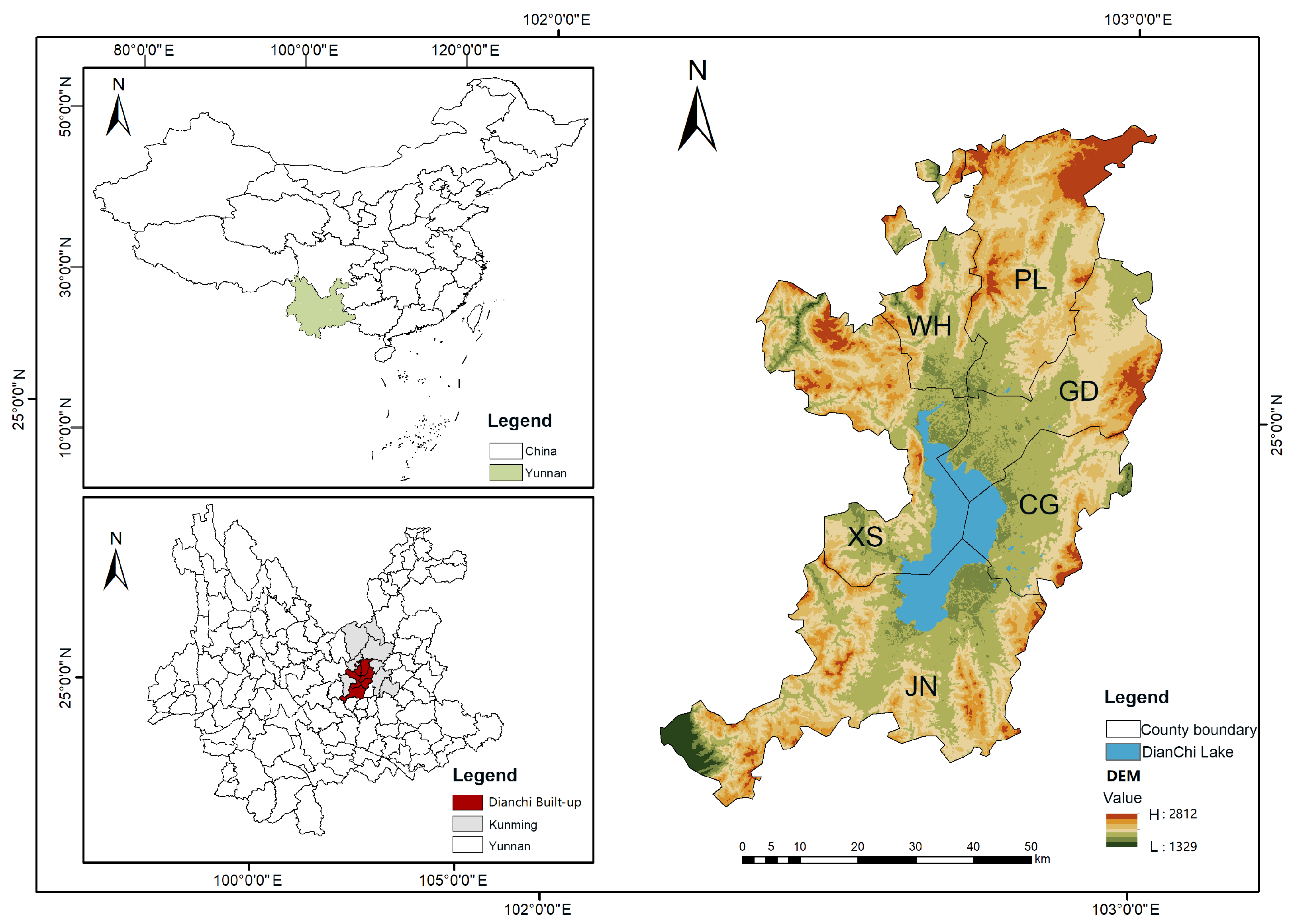
This study takes the urban construction area around Dianchi Lake in Kunming City, Yunnan Province, as the case study (Figure 1). This region is a typical ecologically fragile plateau lake-basin zone, where long-term intensive human activities have encroached upon the lakeshore space, resulting in prominent issues such as natural shoreline retreat and ecological corridor fragmentation. Notably, the proportion of unused land remained at zero throughout 2000–2023, further corroborating the persistence and intensity of anthropogenic disturbance. Wang et al. (2025) [13] conducted an ecological risk assessment of the Dianchi Lake Basin and found that under an economic development scenario permitting unrestricted land-use conversion, the exacerbation of ecological risk was most pronounced, confirming at a macro level the close association between intensive human activities and landscape ecological risk in this region. From the provincial scale to the municipal scale and then to the built-up area around the lake, the land-use structure exhibits a pronounced spatial gradient (see

Table 1. Comparison of land-use composition across Yunnan Province, Kunming City, and the Dianchi Lake Basin (2023).

Region	Total Survey Area (×104 ha)	Cropland (%)	Forestland (%)	Grassland (%)	Built-Up and Industrial Land (%)	Water Bodies (%)
Yunnan Province	3831.93	13.80	65.16	3.42	2.88	1.65
Kunming Municipality	210.13	18.23	53.60	5.91	7.23	2.96
Dianchi Lake Basin	45.97	15.53	42.94	17.34	16.82	7.35

Note: Data sources: Yunnan Provincial Statistical Yearbook (2023); Resource and Environmental Science and Data Center (RESDC), Chinese Academy of Sciences. Table 1 reports the area of the Dianchi Lake Basin (45.97 × 10⁴ ha) based on the Yunnan Provincial Statistical Yearbook (2023). The study area used in this analysis (45.58 × 10⁴ ha) is slightly smaller, covering the six urban districts around Dianchi Lake, and was delineated using GIS based on CAS land-use data.

): The proportion of forestland gradually decreases while that of construction land continuously increases, reflecting the general pattern that the intensity of human activities increases sharply with spatial concentration. Around the lake, urban areas, farmland, and industrial lands are highly intermingled, constituting the underlying spatial basis for landscape fragmentation and ecological risk.

To elucidate the differentiated patterns of landscape ecological risk across ecological sensitivity levels, this study developed a “dual-coupling” analytical framework that integrates (i) land-use composition with ecological sensitivity and (ii) landscape pattern indices with ecological sensitivity. The Analytic Hierarchy Process (AHP) was employed to determine factor weights, and a weighted overlay analysis was conducted to classify ecological sensitivity into five levels [21,22]: non-sensitive (Level 1), low sensitivity (Level 3), moderate sensitivity (Level 5), high sensitivity (Level 7), and extreme sensitivity (Level 9). Based on 2023 land-use data and selected landscape pattern indices, the entropy weight method (EWM) was applied to objectively assign weights to construct the Landscape Ecological Risk Index (LERI) [23,24]. Pearson and Spearman correlation coefficients were then employed for correlation analysis [25,26], while ridge regression (λ = 0.1) [27] and partial least squares regression (PLSR) [28] were used to identify key explanatory land-use factors of LERI. Notably, Li et al. (2025) successfully applied ridge regression in a landscape ecological risk study of the Huaihe River Basin, directly supporting the applicability of this method in the present study [27]. A conceptually similar dual-indicator logic has been applied in vulnerability assessments of the North-Eastern Ecuadorian Amazon [29], reinforcing the methodological basis of the dual-framework approach adopted here.

Based on the above framework, this study aims to address two core questions: Do landscape ecological risks differ significantly across ecological sensitivity levels? Is it possible that low-sensitivity zones exhibit higher risk levels due to specific land-use configurations? Accordingly, we postulate that low-sensitivity zones may display elevated landscape ecological risk, with cropland and grassland serving as the primary positive explanatory factors and construction land as the primary negative explanatory factor. To test these hypotheses, the framework incorporates three methodological provisions: (i) stratified analysis by ecological sensitivity levels to effectively circumvent the interference of spatial autocorrelation in risk factor identification; (ii) objective weighting of landscape pattern indices via the entropy weight method to enhance the robustness of the LERI; and (iii) cross-validation of explanatory factors using two multivariate methods—ridge regression and partial least squares regression (PLSR)—to strengthen the reliability of the identified explanatory relationships.

2. Materials and Methods

2.1. Study Area

The study area is located in the urban construction region around Dianchi Lake in Kunming City, Yunnan Province (Figure 1), with geographical coordinates ranging from 24°29′ N to 25°28′ N and 102°29′ E to 103°01′ E. The average elevation is approximately 1887 m, with considerable elevational variation (1500–2800 m), characterizing this region as a typical ecologically fragile plateau lake-basin zone. Administratively, the study area encompasses the main urban core districts of Kunming—Panlong (PL), Wuhua (WH), Xishan (XS), and Guandu (GD)—as well as the key urban expansion districts of Chenggong (CG) and Jinning (JN). This region features the highest population density and the most intensive economic activities in Yunnan Province. The core water body, Dianchi Lake, covers approximately 309 km², with urban areas, farmland, and industrial lands highly concentrated along its lakeshore. Owing to the fragmented plateau lake-basin topography and the scarcity of flat, developable land, development activities have long encroached upon the lakeshore zone, resulting in natural shoreline retreat, ecological corridor fragmentation, and aggravated non-point source pollution, which collectively exert continuous stress on the water environment of Dianchi Lake and regional ecological security. The CAS land-use classification scheme used in this study includes an “unused land” category (including sandy land, gobi, saline-alkali land, bare land, rocky land, etc.). Interpretation results for all four periods (2000, 2010, 2020, and 2023) show zero unused land within the study area. This is consistent with the actual condition of the Dianchi Lake region, where land resources are under intense pressure from sustained urbanization and agricultural activities, and virtually all land has been utilized—either as construction land, cropland, forest, grassland, or water bodies. The persistent absence of unused land further corroborates the intensity of anthropogenic disturbance described above.

Based on an analysis integrating data from the Yunnan Statistical Yearbook and 2023 land-use remote sensing interpretation results, the land-use structure of the Dianchi Lake Basin exhibits a pronounced gradient characterized by intensifying human activity from the provincial to the basin scale (Table 1). Forestland is the dominant land-use type in Yunnan Province, accounting for 65.16% of the province’s total land area, establishing its role as the core foundation of the ecological security barrier in Southwest China. However, this dominant proportion decreases markedly as the spatial scale narrows—falling to 53.60% at the municipal level and further to 42.94% within the Dianchi Lake Basin. Conversely, the proportion of urban, rural, and industrial land increases sharply from the provincial to the basin scale—its share within the Dianchi Lake Basin (16.82%) is 2.3 times that of Kunming City (7.23%) and 5.8 times that of Yunnan Province (2.88%). The proportions of cropland and grassland also exhibit increasing trends. This gradient directly reflects the general pattern that the intensity of human activities increases sharply with spatial concentration, while the natural ecological foundation is correspondingly compressed. The lakeshore area serves as a concentrated distribution zone for urban areas, farmland, and industrial lands, where construction, agricultural, and ecological spaces are highly intermingled and intensely competitive.

2.2. Data Sources and Preprocessing

Land-use data spanning four periods (2000, 2010, 2020, and 2023) were obtained from the Resource and Environmental Science and Data Center (RESDC) of the Chinese Academy of Sciences (CAS). These data were derived from Landsat TM/ETM+/OLI satellite imagery via supervised classification at a spatial resolution of 30 m. The land-use types were classified into five categories: cropland, forestland, grassland, water bodies, and construction land. These datasets were utilized to: (i) provide the land-use factor required for ecological sensitivity evaluation; (ii) construct land-use transfer matrices and identify evolutionary trajectories; and (iii) calculate landscape pattern indices. Both the ecological sensitivity evaluation and the landscape pattern index calculations were based on the 2023 baseline year. The Normalized Difference Vegetation Index (NDVI) was derived via the Google Earth Engine (GEE) platform; specifically, Landsat series imagery was subjected to radiometric calibration, atmospheric correction, cloud masking, and annual maximum value compositing to generate annual NDVI data at a 30 m spatial resolution. The Digital Elevation Model (DEM) was acquired from the ASTER GDEM V3 product (30 m spatial resolution) to extract topographic factors, including elevation and slope. Road and water network data for buffer analysis were sourced from the 2023 version of OpenStreetMap (OSM). Finally, all spatial data were uniformly resampled to a 30 m resolution and projected to the WGS_1984_UTM_Zone_48N coordinate system.

2.3. Method

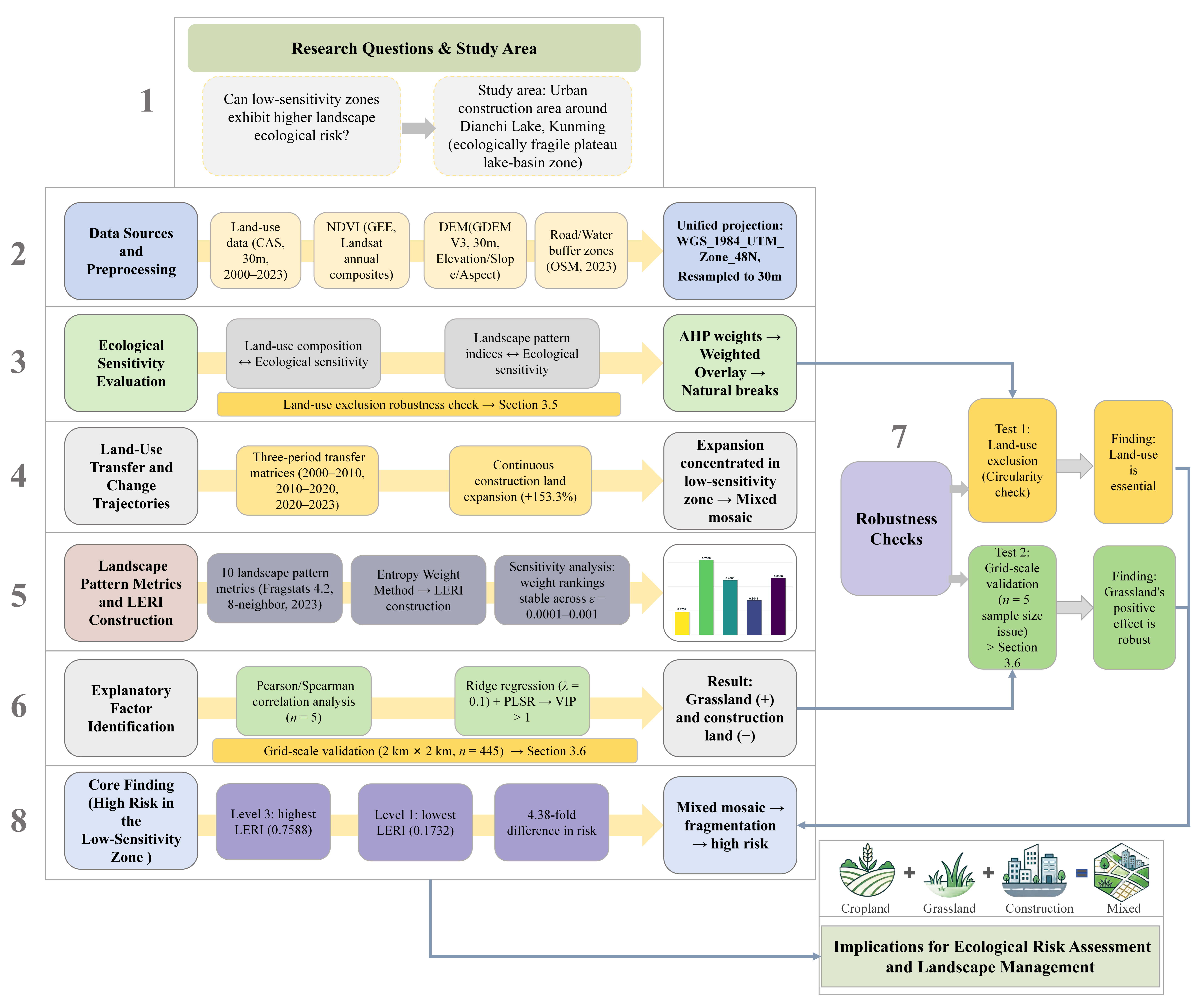
The methodological framework of this study was organized around three progressive steps: hierarchical classification, risk quantification, and driver identification. For the evaluation phase, seven factors were selected to construct an ecological sensitivity index system. The Analytic Hierarchy Process (AHP) was employed to establish the judgment matrix and determine factor weights (consistency ratio CR < 0.1), and a weighted overlay analysis was conducted to classify the study area into five ecological sensitivity levels (1, 3, 5, 7, and 9, corresponding to non-sensitive, low sensitivity, moderate sensitivity, high sensitivity, and extreme sensitivity, respectively). On this basis, ten landscape pattern indices were calculated in the Fragstats software (version 4.2) using 2023 land-use data, and the entropy weight method was applied to construct the Landscape Ecological Risk Index (LERI). The land-use composition within each sensitivity level was summarized via ArcGIS 10.8 overlay, and land-use transfer matrices for three periods (2000–2010, 2010–2020, and 2020–2023) were compiled to trace the temporal trajectories of land-use conversion. For the driver identification phase, Pearson and Spearman correlation analyses, ridge regression (λ = 0.1), and partial least squares regression (PLSR) were applied to identify the key land-use explanatory factors of LERI, with a particular focus on elucidating the mechanism by which landscape fragmentation drives the anomalously elevated risk within the low-sensitivity zone (Figure 2). To further validate the robustness of the analytical framework, two complementary checks were conducted: (i) a land-use exclusion test to examine potential circularity in the sensitivity classification, and (ii) a grid-scale validation to assess the consistency of the explanatory factors identified at the sensitivity-level scale.

2.3.1. Ecological Sensitivity Indicator System Construction and Level Classification

Seven factors were selected for the ecological sensitivity evaluation: land use, elevation, slope, aspect, NDVI, water buffer, and road buffer. Based on their attributes, these factors were categorized into four groups: topography, vegetation, water systems, and anthropogenic disturbance. The topographic group comprises elevation, slope, and aspect, all derived from the DEM, to capture the fundamental control of terrain on the spatial differentiation of ecosystems. The vegetation group is represented by NDVI, which characterizes land surface cover and growth conditions. The water systems group is represented by water buffer zones, constructed as the Euclidean distance from water bodies, delineating the sphere of ecological influence of water. The anthropogenic disturbance group incorporates both land use and the road buffer—land use serves as a spatial proxy for human development intensity, while the road buffer reflects the disturbance pressure imposed by transportation accessibility.

To determine the weights, seven experts spanning urban planning, ecology, landscape ecology, plant ecology, social-ecological systems, and environmental management (see Table S1C for details) were invited to conduct pairwise comparisons of the relative importance of each factor using Saaty’s 1–9 scale. All individual judgment matrices passed the consistency test (CR < 0.1), and the aggregated matrix also satisfied the consistency requirement (CR = 0.0126 < 0.1; Table S1B). The geometric mean method—where the aggregated value is calculated as (a1 × a2 × … × an)1/n, with n being the number of experts and ai representing the corresponding judgment values—was then applied to integrate the individual expert judgments into a single composite judgment matrix. The principal eigenvector of this matrix was then calculated and normalized to yield the final weights for each factor: elevation (0.0841), slope (0.1806), aspect (0.0861), land use (0.2424), NDVI (0.1568), water buffer (0.1589), and road buffer (0.0911). The classification criteria and assigned weights for each factor are detailed in

Table 2. Classification criteria and weights of ecological sensitivity assessment indicators.

Factor	Assignment Basis	Non-Sensitive (1)	Low Sensitivity (3)	Moderate Sensitivity (5)	High Sensitivity (7)	Extreme Sensitivity (9)	Weight
Elevation (m)	Altitude	≤1500	1500–1800	1800–2000	2000–2800	≥2800	0.0841
Slope (°)	Terrain gradient	≤8°	8–15°	15–25°	25–35°	≥35°	0.1806
Aspect	Orientation	Flat, South	Southeast, Southwest	East, West	Northeast, Northwest	North	0.0861
Land-use type	Land-use category	Unused land	Construction land	Cropland	Forestland, Grassland	Water bodies	0.2424
NDVI	Vegetation index value	≤0.2	0.2–0.4	0.4–0.6	0.6–0.8	≥0.8	0.1568
Water buffer distance (m)	Distance to water bodies	≥800	500–800	200–500	50–200	≤50	0.1589
Road buffer distance (m)	Distance to roads	≥500	300–500	100–300	30–100	≤30	0.0911

Note: Weights sum to 1.0000 (rounded to four decimal places). Notably, unused land accounted for 0% of the study area throughout 2000–2023, indicating that the non-sensitive category for the land-use factor was virtually absent within the study area during the assessment period.

. Finally, within the ArcGIS 10.8 environment, a weighted linear overlay was applied to calculate the ecological sensitivity index for each pixel. The natural breaks method was then used to classify the results into five sensitivity levels—non-sensitive, low sensitivity, moderate sensitivity, high sensitivity, and extreme sensitivity—thereby generating the spatial distribution map of ecological sensitivity.

Importantly, the land-use factor, despite having the highest AHP weight (0.2424), effectively operates on only four sensitivity levels within the study area. This is because the “non-sensitive” (Level 1) class for this factor is never assigned—unused land remained absent throughout the 2000–2023 period. However, this does not compromise the utility of the land-use factor as a key discriminator; the distinctions among the five represented classes (cropland, forest, grassland, water bodies, and construction land) remain meaningful and contribute substantially to the overall sensitivity classification. Moreover, the remaining six factors (elevation, slope, aspect, NDVI, water buffer, and road buffer) continue to provide differentiation across all five sensitivity levels, ensuring that the final five-level classification derived from the composite index remains valid and informative.

To further examine potential circularity in the sensitivity classification—where land use contributes to both the zoning procedure and the LERI—we also re-derived the ecological sensitivity zones following the same procedure as above, but with the land-use factor excluded and the remaining six weights re-normalized. The results of this robustness check are presented in Section 3.5.

2.3.2. Landscape Pattern Metrics and LERI Calculation

Landscape pattern indices were calculated based on 2023 land-use data using Fragstats 4.2 software with the 8-neighbor rule, taking each ecological sensitivity level (1, 3, 5, 7, and 9) as the analytical unit. A total of ten landscape pattern indices were selected (

Table 3. Landscape pattern metrics and their ecological implications.

Metric	Abbreviation	Unit	Ecological Implication
Number of patches	NP	count	Indicates the degree of landscape subdivision. An increase in NP, especially for natural patches (e.g., forest and grassland), signals the dissection of continuous habitats into scattered units.
Patch density	PD	n/100 ha	Number of patches per unit area. Higher values reflect greater landscape fragmentation.
Largest patch index	LPI	%	Reflects the proportion of total landscape area occupied by the largest patch. A decline in LPI for forest or grassland signals shrinking core habitat extent and loss of structural dominance.
Edge density	ED	m/ha	Higher values indicate deeper dissection of patches by boundaries, resulting in more disturbed edge zones and less undisturbed core habitat.
Contagion index	CONTAG	%	Low values indicate a landscape composed of numerous small patches with low connectivity; high values suggest the presence of well-connected dominant patches.
Aggregation index	AI	%	High values indicate a landscape dominated by fewer, larger patches; low values indicate dispersed, fine-grained patch distribution.
Proportion of like adjacencies	PLADJ	%	Measures the degree of adjacency among patches of the same type. A decline indicates increasing enclosure by dissimilar land-use types (e.g., built-up land and cropland), intensifying spatial isolation.
Patch cohesion index	COHESION	—	Directly measures the physical connectedness of patches. Lower values reflect reduced spatial continuity and aggregation of a given patch type.
Interspersion and juxtaposition index	IJI	%	Captures the degree of intermixing among different patch types. Low values for a given type indicate adjacency to only a limited range of other types, signaling a higher risk of spatial isolation.
Shannon’s diversity index	SHDI	—	Reflects landscape-type richness and evenness. In human-dominated landscapes, elevated SHDI may result from the encroachment of construction land into natural land-use types rather than representing ecologically beneficial diversification.

): Number of Patches (NP), Patch Density (PD), Largest Patch Index (LPI), Edge Density (ED), Contagion Index (CONTAG), Percentage of Like Adjacencies (PLADJ), Interspersion and Juxtaposition Index (IJI), Patch Cohesion Index (COHESION), Shannon’s Diversity Index (SHDI), and Aggregation Index (AI). Among these, eight indices—NP, PD, LPI, ED, PLADJ, IJI, COHESION, and AI—were computed at the class level to quantify the spatial configuration characteristics of different land-use types within each sensitivity level, reflecting differences in fragmentation, aggregation, and connectivity among cropland, forestland, grassland, water bodies, and construction land at the patch scale. CONTAG and SHDI were computed at the landscape level to measure the contagion and diversity of the overall landscape mosaic for each sensitivity level, independent of specific land-use types. Class-level indices provide detailed information on the contribution of different land-use types to landscape fragmentation, while landscape-level indices capture the comprehensive pattern characteristics of each sensitivity level as a whole.

The Landscape Ecological Risk Index (LERI) was constructed using the entropy weight method (EWM). To eliminate the effects of different dimensionalities, each landscape index was first normalized using min-max normalization. Based on their directional contribution to ecological risk, NP, PD, ED, IJI, and SHDI were identified as positive indicators (where higher values indicate higher risk), while LPI, CONTAG, PLADJ, COHESION, and AI were identified as negative indicators (where lower values indicate higher risk). The normalization formulas are as follows:

$${\mathrm{For} \mathrm{positive} \mathrm{indicators}: p}_{ij}={\displaystyle \frac{x_{ij}-\min (x_j)}{\max (x_j)-\min (x_j)}}+\epsilon$$

(1)

$$\mathrm{For} \mathrm{negative} \mathrm{indicators}: p_{ij}={\displaystyle \frac{\max (x_j)-x_{ij}}{\max (x_j)-\min (x_j)}}+\epsilon$$

(2)

where $\epsilon = 0.0001$ is a small constant introduced to avoid zero values.

The proportion of the $i$-th sensitivity level for the $j$-th metric was calculated as follows:

$$r_{ij}={\displaystyle \frac{p_{ij}}{{\sum }_{i=1}^m{p}_{ij}}}$$

(3)

The entropy value of the $j$-th metric was then calculated as follows:

$$e_j=-{\displaystyle \frac{1}{\ln m}}{\displaystyle \sum _{i=1}^m}{r}_{ij}\ln r_{ij}$$

(4)

where $\mathrm{m}$ denotes the number of sensitivity levels $(m = 5)$.

The differentiation coefficient was obtained as follows:

$$d_j=1-e_j$$

(5)

The weight of each metric was determined by the following:

$$w_j={\displaystyle \frac{d_j}{{\sum }_{j=1}^n{d}_j}}$$

(6)

where $n = 10$ is the number of landscape pattern metrics.

Finally, the LERI value for each sensitivity level was obtained as the weighted sum of the normalized metric scores:

$${\mathrm{LERI}}_i={\sum }_{j=1}^n{w}_j·p_{ij}$$

(7)

The entropy weight calculations were performed using R version 4.5.3 via custom scripts, ensuring full reproducibility.

Sensitivity analysis: To assess the robustness of the entropy weight results with respect to the normalization parameter ε, we calculated the weights and LERI values under three different ε levels (0.0001, 0.0005, and 0.001), and also compared the min-max normalization scheme without ε. The results show that the weight rankings remain identical across all tested conditions (COHESION > IJI > ED > NP > PD > LPI > SHDI > CONTAG > AI > PLADJ), and the LERI rankings across the five sensitivity levels also remain unchanged (low sensitivity > extreme sensitivity > moderate sensitivity > high sensitivity > non-sensitive). These results confirm that both the entropy weights and the LERI rankings are insensitive to the choice of ε and to the normalization bounds, indicating that the risk ranking across sensitivity levels is robust and not driven by specific parameter settings.

LERI values were compared across the five sensitivity levels to determine their relative ranking). Because LERI is a dimensionless composite indicator whose absolute values do not carry universal risk threshold meanings, this study adopts relative comparisons to interpret the ordinal differences across levels.

2.3.3. Land-Use Composition and Transfer Analysis

Within the ArcGIS 10.8 environment, the 2023 ecological sensitivity zoning map was overlaid with the land-use map of the same year to calculate the area percentages of cropland, forestland, grassland, water bodies, and construction land within each sensitivity level (1, 3, 5, 7, and 9). Concurrently, using the four-period land-use data (2000, 2010, 2020, and 2023), land-use transfer matrices were constructed for three intervals (2000–2010, 2010–2020, and 2020–2023) to track long-term dynamics such as construction land expansion and cropland reduction. Conducted independently of the calculation of landscape pattern indices and the LERI, this overlay analysis was designed to reveal the replacement process of semi-natural matrices by construction land, thereby providing quantitative evidence to decipher the historical explanatory factors of landscape fragmentation within the low-sensitivity zone. The land-use transfer matrix is expressed as follows:

$$\mathrm{N}=\left(\begin{array}{cccc}{n}_{11}& n_{12}& \dots & n_{1m}\\ n_{21}& n_{22}& \dots & n_{2m}\\ ⋮& ⋮& \ddots & ⋮\\ n_{m1}& n_{m2}& \dots & n_{mm}\end{array}\right)$$

(8)

2.3.4. Identification of Land-Use Explanatory Factors

All statistical analyses were performed using R version 4.5.3 with the glmnet and pls packages. Pearson correlation and Spearman rank correlation coefficients were employed to assess linear and monotonic relationships, respectively, between the proportion of each land-use type and the Landscape Ecological Risk Index (LERI).

The Pearson correlation coefficient r is calculated as follows:

$$\mathrm{r}={\displaystyle \frac{{\sum }_{i=1}^n(x_i-\overline{x}\left)\right(y_i-\overline{y})}{\sqrt{{\sum }_{i=1}^n(x_i-\overline{x}{)}^2\cdot {\sum }_{i=1}^n(y_i-\overline{y}{)}^2}}}$$

(9)

where $x_i$ and $y_i$ are the individual sample values, $\overline{x}$ and $\overline{y}$ are the respective means, and $\mathrm{n}$ is the number of samples (here, n = 5 ecological sensitivity levels).

The Spearman’s rank correlation coefficient $\rho$ is defined as follows:

$$\mathsf{\rho }=1-{\displaystyle \frac{6{\sum }_{i=1}^n{d}_i^2}{n(n^2-1)}}$$

(10)

where $d_i=\mathrm{rank}(x_i)-\mathrm{rank}(y_i)$ is the difference between the ranks of the two variables for the $i$-th sample.

To address multicollinearity among independent variables, all variables were first standardized (mean = 0, SD = 1) prior to model fitting. Ridge regression was then applied to estimate the regression coefficients, with the penalty parameter fixed at λ = 0.1. Ridge regression solves for coefficients by minimizing the following loss function:

$${\hat{\mathsf{\beta }}}^{\mathrm{ridge}}=\arg \underset{\beta }{\min }\left\{{\sum }_{i=1}^n{\left(y_i-{\beta }_0-{\sum }_{j=1}^p{x}_{ij}{\beta }_j\right)}^2+\lambda {\sum }_{j=1}^p{\beta }_j^2\right\}$$

(11)

where $p = 5$ denotes the number of land-use types (cropland, forestland, grassland, water bodies, and construction land), and ${\beta }_j$ represents the regression coefficient for each type. The penalty parameter was fixed at λ = 0.1. Due to the limited sample size at the sensitivity-level scale (n = 5), cross-validation for λ selection was not feasible. To validate the stability of the coefficient signs, we examined the coefficient paths across a range of λ values using grid-scale data (see “Grid-scale validation” below). Because all variables were standardized prior to model fitting, the estimated coefficients are directly interpretable as standardized regression coefficients, enabling direct comparison of the relative contributions of different land-use types to LERI.

As a robustness check, partial least squares regression (PLSR) was further employed. The number of latent variables was set to one, as determined via leave-one-out cross-validation. We acknowledge that applying PLSR with a single latent variable to five sensitivity-level observations is near degenerate and does not support robust inferential claims. The PLSR results presented here are therefore intended solely as an exploratory assessment of directional consistency, not as confirmatory causal identification. Standardized regression coefficients and variable importance in projection (VIP) scores were then calculated. The VIP score for the j-th independent variable is defined as follows:

$${\mathrm{VIP}}_j=\sqrt{{\displaystyle \frac{p{\sum }_{k=1}^m{w}_{kj}^2\cdot {\mathrm{SSY}}_k}{{\sum }_{k=1}^m{\mathrm{SSY}}_k}}}$$

(12)

where $p$ is the number of independent variables, $m$ is the number of latent variables extracted (here, m = 1), $w_{kj}$ is the weight of the $j$-th variable on the $k$-th latent variable, and ${\mathrm{SSY}}_k$ is the sum of squares of the dependent variable explained by the $k$-th latent variable. It is commonly accepted that variables with VIP > 1 are considered to possess significant explanatory importance.

Grid-scale validation: To assess the robustness of the explanatory factors identified at the sensitivity-level scale (n = 5), we additionally conducted a validation using a 2 km × 2 km regular fishnet grid across the study area, yielding 445 valid grid cells after removing cells with missing data. For each grid cell, we calculated the ten landscape pattern metrics and LERI using the same entropy weights as in the sensitivity-level analysis. Each grid cell was then assigned to its corresponding ecological sensitivity level based on the 2023 sensitivity zonation. Pearson and Spearman correlation analyses, ridge regression (λ = 0.1), and PLSR with VIP calculation were then repeated at the grid scale. The results of this validation are presented in Section 3.6.

3. Results

3.1. Spatial Distribution of Ecological Sensitivity

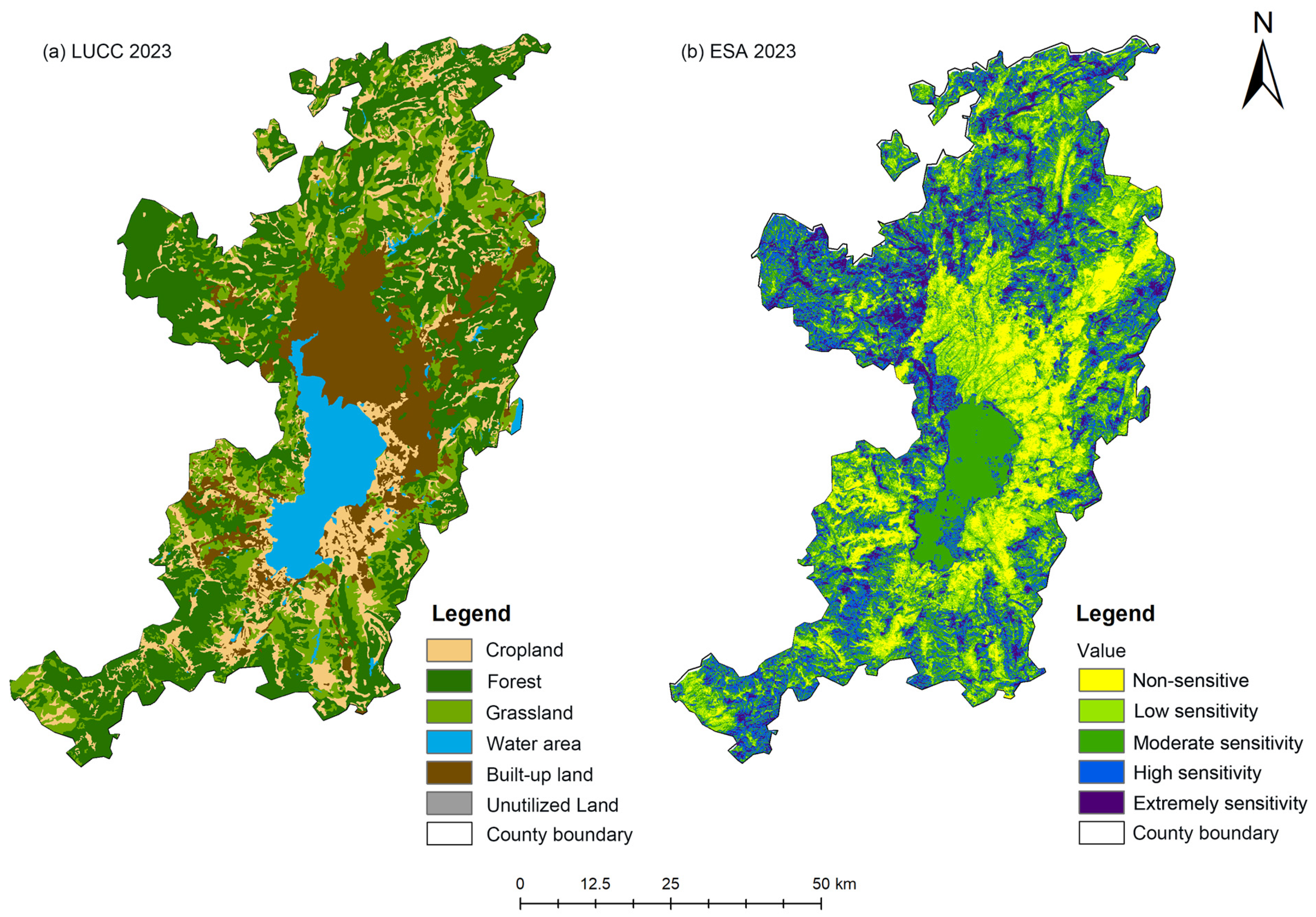
The ecological sensitivity classification statistics and spatial distribution of the study area are presented in

Table 4. Statistical summary of ecological sensitivity levels in the study area (2023).

Sensitivity Level	Assigned Value	Ecological Sensitivity Index Range	Area (×104 ha)	Proportion (%)
Non-sensitive	1	1.4106–2.2103	5.08	11.14
Low sensitivity	3	2.2103–2.5988	10.10	22.16
Moderate sensitivity	5	2.5988–2.9307	15.09	33.10
High sensitivity	7	2.9307–3.2625	11.42	25.06
Extreme sensitivity	9	3.2625–4.4271	3.89	8.54
Total	—	—	45.58	100.00

Note: Area data were derived from spatial statistics within the ArcGIS 10.8 environment; proportions are rounded to two decimal places.

and Figure 3. The area of each sensitivity level followed a descending order of moderate sensitivity > high sensitivity > low sensitivity > non-sensitive > extreme sensitivity. The moderate-sensitivity zone (Level 5) occupied the largest area, covering 15.09 × 10⁴ ha and accounting for 33.10% of the total study area, followed by the high-sensitivity zone (Level 7), which represented 25.06%. Together, these two zones comprised over 58% of the study area, indicating that the overall ecological baseline of the region is relatively fragile. The low-sensitivity zone (Level 3) and the non-sensitive zone (Level 1) together accounted for approximately 33% of the total area, mainly distributed across densely urbanized lakeside areas. The extreme-sensitivity zone (Level 9) occupied the smallest proportion at only 8.54%, predominantly concentrated within the water body of Dianchi Lake and its lakeshore wetlands.

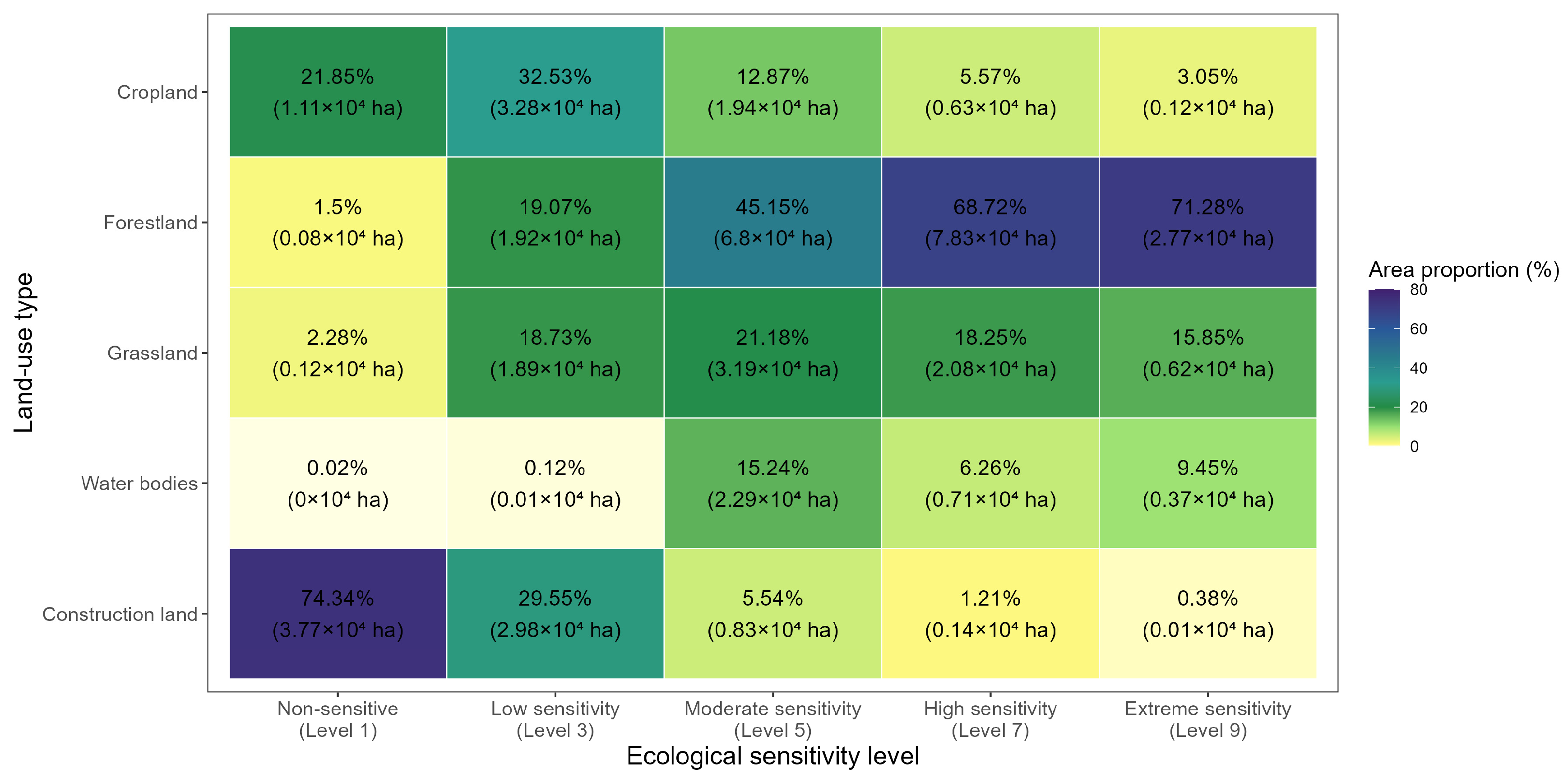
The land-use composition within each ecological sensitivity level exhibited pronounced spatial differentiation (Figure 4). The non-sensitive zone (Level 1) was overwhelmingly dominated by construction land (74.34%), followed by cropland (21.85%). The low-sensitivity zone (Level 3) displayed the most balanced composition, with cropland (32.53%), construction land (29.55%), and grassland (18.73%) constituting a typical cropland–construction land–grassland mixed mosaic. In the moderate-sensitivity zone (Level 5), forestland increased to 45.15%, while grassland (21.18%) and cropland (12.87%) retained notable proportions, and water bodies accounted for 15.24%. The high-sensitivity zone (Level 7) and extreme-sensitivity zone (Level 9) were overwhelmingly dominated by forestland (68.72% and 71.28%, respectively), with cropland and construction land together comprising less than 6% of each zone. Along the gradient from non-sensitive to low sensitivity, moderate sensitivity, high sensitivity, and extreme sensitivity, the proportion of construction land decreased gradually from 74.34% to 0.38% and cropland declined from its peak in the low-sensitivity zone (32.53%) to 3.05%, while forestland dominance correspondingly increased from 1.50% to 71.28%. Notably, the low-sensitivity zone was the only level in which cropland, grassland, and construction land each exceeded 15%, indicating the highest degree of spatial heterogeneity and landscape intermixing within the study area.

3.2. Landscape Pattern Metrics and LERI

The ten landscape pattern indices for each ecological sensitivity level are presented in

Table 5. Landscape pattern indices across ecological sensitivity levels (2023).

Sensitivity Level	NP	PD	LPI	ED	CONTAG	PLADJ	IJI	COHESION	SHDI	AI
Non-sensitive (1)	22,713	40.89	5.57	19.61	74.54	83.40	66.72	96.31	0.71	83.47
Low sensitivity (3)	46,281	46.06	15.99	28.85	52.58	69.08	73.03	93.45	1.36	69.23
Moderate sensitivity (5)	46,838	31.14	14.09	21.60	52.64	72.30	65.51	95.57	1.40	72.42
High sensitivity (7)	32,671	28.68	2.68	20.15	66.62	67.84	65.20	92.74	0.96	67.99
Extreme sensitivity (9)	17,932	46.21	1.68	23.37	68.41	66.22	72.61	82.29	0.89	66.36

Note: NP, PD, and ED were calculated via direct summation across land-use types; LPI represents the maximum value among categories. PLADJ, IJI, COHESION, and AI were aggregated as area-weighted averages based on the percentage of landscape (PLAND) of each land-use type. CONTAG and SHDI were directly obtained at the landscape level. All metrics were computed using Fragstats 4.2 with the 8-neighbor rule.

. Across the five sensitivity zones, a clear divergence in landscape structure emerges: the low-sensitivity zone (Level 3) exhibited the highest fragmentation signals—with ED peaking at 28.85 and NP reaching 46,281 (second only to the moderate-sensitivity zone), alongside the lowest CONTAG (52.58%) and AI (69.23%)—indicating that this zone experiences the most severe landscape dissection among all levels. In contrast, the non-sensitive zone displayed a distinctly different pattern, as detailed below.

The non-sensitive zone (Level 1) exhibited a distinctly different landscape pattern. Specifically, NP (22,713) and ED (19.61) were comparatively low, while CONTAG (74.54), PLADJ (83.40), and AI (83.47) were the highest among all levels. Furthermore, LPI (5.57) was markedly lower than that of the low-sensitivity zone, and SHDI (0.71) was the lowest overall. These indices collectively point to a homogenized structure dominated by large contiguous construction land patches, thereby maintaining relatively high landscape integrity.

The low-sensitivity zone (Level 3) exhibited pronounced fragmentation characteristics across multiple indices. Specifically, Edge Density (ED = 28.85) and Interspersion and Juxtaposition Index (IJI = 73.03%) were the highest among the five levels; Number of Patches (NP = 46,281) and Patch Density (PD = 46.06) were also at extremely high levels, ranking only slightly lower than those of the moderate-sensitivity zone (NP = 46,838) and extreme-sensitivity zone (PD = 46.21), respectively. Furthermore, Contagion Index (CONTAG = 52.58%) was the lowest overall, while Percentage of Like Adjacencies (PLADJ = 69.08%) and Aggregation Index (AI = 69.23%) remained at relatively low levels. The consistently high values of positive indicators and low values of negative indicators point to a landscape characterized by fine patches, pronounced edge dissection, and high interspersion among different patch types—consistent with the “cropland–construction land–grassland” mosaic structure identified in Section 3.1. Notably, the Largest Patch Index (LPI = 15.99%) in the low-sensitivity zone was the highest among all levels. Although this may appear to contradict the fragmentation signals described above, it reflects the presence of large contiguous cropland patches that coexist with fine-scale dissection by construction land and grassland patches—a pattern we elaborate further below. This suggests the presence of large contiguous patches (e.g., continuous cropland) despite the overall fragmented context; meanwhile, Patch Cohesion Index (COHESION = 93.45%) also remained at a relatively high level, only slightly lower than that of the non-sensitive zone (96.31) and moderate-sensitivity zone (95.57), indicating that physical connectivity among similar patch types remained relatively robust.

The moderate-sensitivity zone (Level 5) recorded the highest SHDI (1.40) among all levels, followed closely by the low-sensitivity zone (1.36). Combined with the land-use composition presented in Section 3.1, the high diversity within these two levels arises from the coexistence of multiple land-use types, rather than from the inherent richness of natural ecosystems. The high-sensitivity zone (Level 7) and extreme-sensitivity zone (Level 9) were dominated by forestland, yet their LPI values were only 2.68 and 1.68, respectively. Being the lowest among the five levels, this indicates that although forest patches occupy the largest total area, they tend to be dispersed. However, their CONTAG values (66.62 and 68.41, respectively) were second only to that of the non-sensitive zone, suggesting that forest patches still maintained relatively good spatial connectivity. Interestingly, the extreme-sensitivity zone exhibited the lowest COHESION (82.29) among all levels, which may be attributable to the spatial segmentation of forest patches by the water body of Dianchi Lake.

These results indicate that the LERI does not exhibit a monotonic increasing relationship with sensitivity levels; instead, it peaks in the low-sensitivity zone and reaches its minimum in the non-sensitive zone. This nonlinear pattern is closely tied to the land-use composition and landscape configuration across levels, and will be further examined through correlation analysis and regression modeling to identify the key explanatory factors.

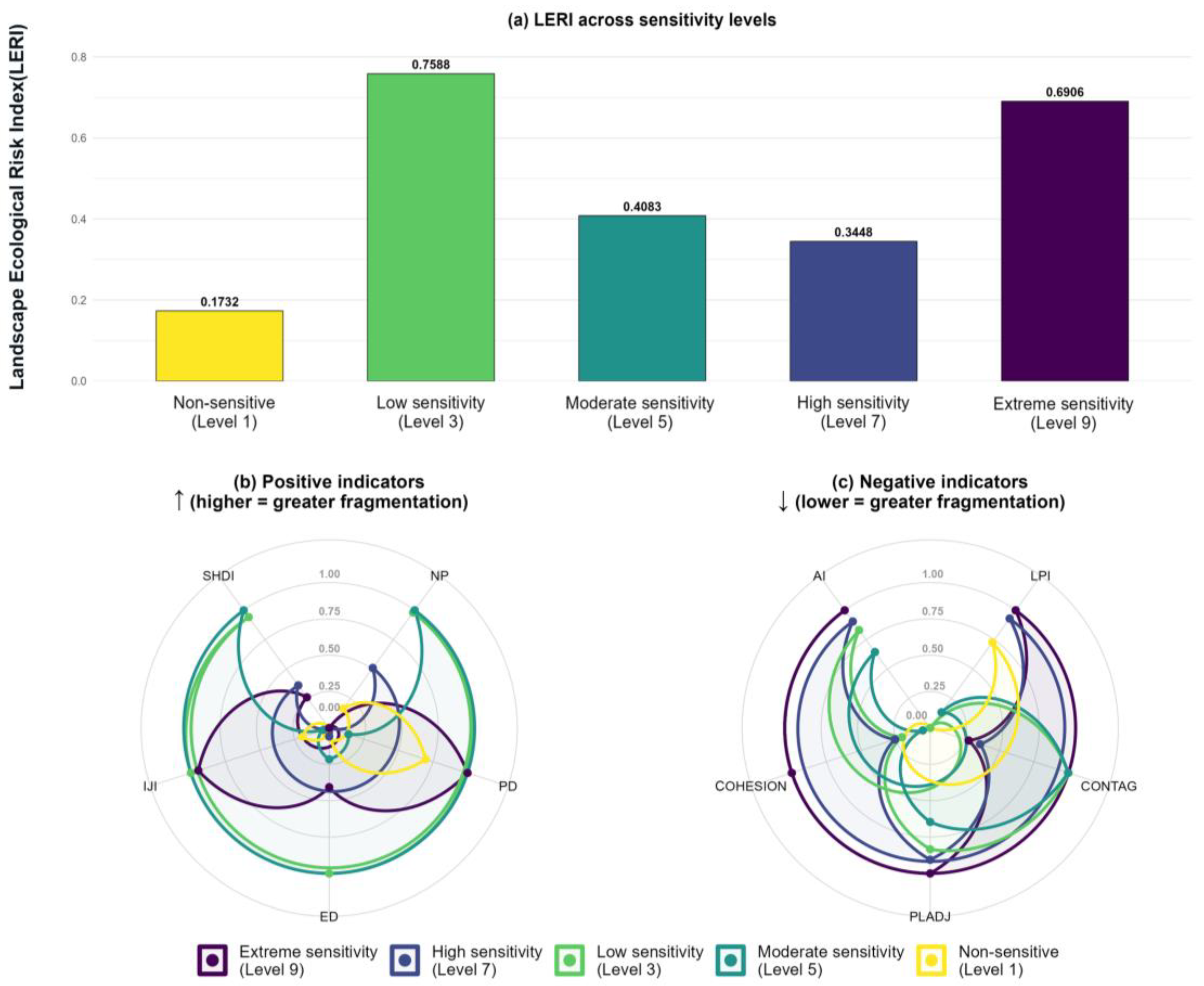
The calculated Landscape Ecological Risk Index (LERI) for each ecological sensitivity level is presented in

Table 6. Assessment and ranking of Landscape Ecological Risk Index (LERI) across ecological sensitivity levels (2023).

Sensitivity Level	Code	LERI Value	Rank
Non-sensitive	1	0.1732	5
Low sensitivity	3	0.7588	1
Moderate sensitivity	5	0.4083	3
High sensitivity	7	0.3448	4
Extreme sensitivity	9	0.6906	2

Note: LERI values were calculated via the entropy weight method based on ten landscape pattern indices (see Section 2.3.2). Higher LERI values indicate greater risk. Bold indicates the maximum value among the five levels. Rank indicates the relative ordering of LERI across the five sensitivity levels (1 = highest, 5 = lowest). As LERI is a dimensionless composite indicator whose absolute values do not carry universal risk threshold meanings, this study adopts relative comparisons among levels to assign risk categories.

. The low-sensitivity zone (Level 3) exhibited the highest LERI value (0.7588), while the non-sensitive zone (Level 1) recorded the lowest (0.1732). The LERI values for the moderate-sensitivity (Level 5), high-sensitivity (Level 7), and extreme-sensitivity (Level 9) zones were 0.4083, 0.3448, and 0.6906, respectively. The LERI displayed a fluctuating trend of an initial increase, subsequent decrease, and then a renewed increase along the gradient of sensitivity levels, with the peak in the low-sensitivity zone being particularly pronounced. These results indicate that the LERI does not exhibit a linear correspondence with sensitivity levels—the low-sensitivity zone represents the area with the highest landscape ecological risk within the study area, whereas the non-sensitive zone exhibits the lowest risk.

Figure 5 Landscape ecological risk and landscape pattern along the ecological sensitivity gradient. Figure 5a. Landscape Ecological Risk Index (LERI) for each ecological sensitivity level. Figure 5b,c. Radar charts of positive and negative indicators, respectively. The radar charts reveal the landscape structural basis underlying the risk peak. All indices presented are directionally transformed standardized scores (0–1), with higher scores indicating a greater contribution to landscape ecological risk. For positive indicators (NP, PD, ED, IJI, and SHDI), higher original values correspond to higher scores; for negative indicators (LPI, CONTAG, PLADJ, COHESION, and AI), lower original values translate into higher scores after directional transformation. Original landscape metric values are presented in Table 5, and standardized scores are provided in Table S3.

Among the positive indicators (NP, PD, ED, IJI, and SHDI), the low-sensitivity zone approached the outer edge of the radar chart across multiple metrics. Specifically, ED (1.000) and IJI (1.000) were the highest among the five levels, while NP (0.981) and PD (0.991) also reached extremely high levels, ranking only slightly lower than those of the moderate-sensitivity and extreme-sensitivity zones, respectively. This configuration reflects a fragmentation pattern characterized by numerous patches, extremely high density, pronounced edge dissection, and intensive interspersion among different land-use types. Conversely, the non-sensitive zone recorded the lowest values for both ED (0.000) and SHDI (0.000), indicating a relatively intact landscape. Furthermore, the highest SHDI value occurred in the moderate-sensitivity zone (1.000), followed closely by the low-sensitivity zone (0.942).

Among the negative indicators (LPI, CONTAG, PLADJ, COHESION, and AI), the low-sensitivity zone exhibited the highest standardized score for CONTAG (1.000), indicating the lowest landscape contagion and the highest interspersion among patch types. Furthermore, PLADJ (0.834) and AI (0.832) occupied relatively outer positions on the radar chart, suggesting relatively weak adjacency and aggregation among similar patch types. The LPI in the low-sensitivity zone was closest to the center of the radar chart (standardized score = 0.000, the lowest among the five levels). The CONTAG score for the low-sensitivity zone was the highest after directional transformation (1.000), corresponding to the lowest raw contagion value. It should be noted that the original LPI value (15.99%) in the low-sensitivity zone was the highest among the five levels (Table 5)—this does not contradict its innermost position in the radar chart. Because the chart displays directionally transformed standardized scores (0–1), higher original values for negative indicators correspond to lower transformed scores, thus positioning them closer to the center. Conversely, the non-sensitive zone exhibited most of these negative indicators (such as CONTAG, PLADJ, COHESION, and AI) near the center of the radar chart (scores of 0.000). This central positioning perfectly reflects its homogenized structure dominated by contiguous construction land, as its high original structural integrity translates to the lowest standardized risk scores.

These collective patterns point to a core finding: the peak of landscape fragmentation does not occur in the high-sensitivity zones, but rather is concentrated in the low-sensitivity zone. The systematic outward expansion of positive indicators and the inward contraction of negative indicators in the low-sensitivity zone collectively drive its LERI to the peak value (0.7588), making it the area with the highest landscape ecological risk within the study area. Conversely, the non-sensitive zone exhibits the lowest risk (0.1732) due to landscape homogenization. The LERI of the low-sensitivity zone is 4.38 times that of the non-sensitive zone. This counterintuitive, nonlinear pattern provides the crucial structural foundation for the subsequent identification of driving factors and discussion of underlying mechanisms.

3.3. Land-Use Composition and Change Trajectories

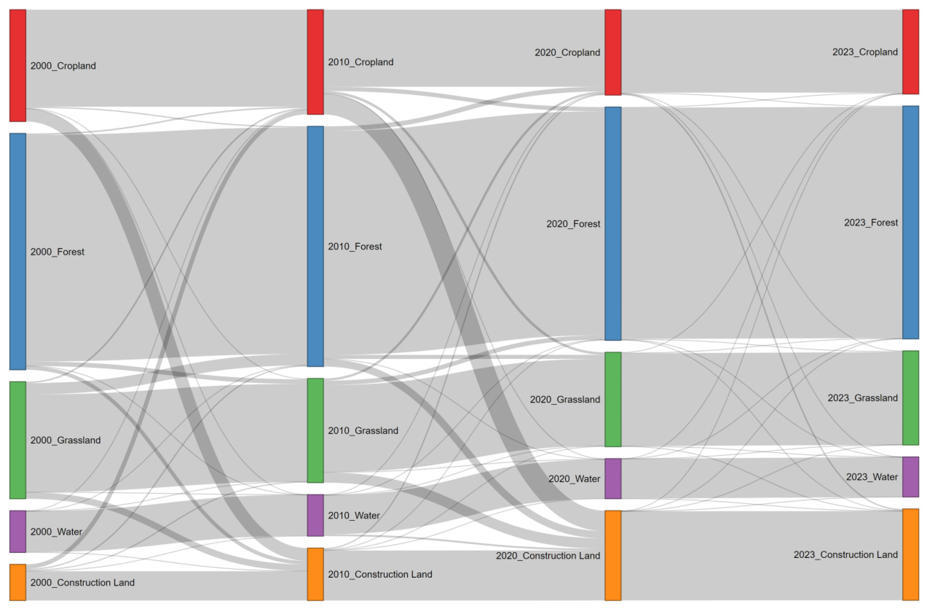
Land-use changes across the three periods from 2000 to 2023 are summarized in

Table 7. Land-use changes across three periods (2000–2023).

Period	Land-Use Type	Initial Area (×104 ha)	Net Change (×104 ha)	Change Rate (%)
2000–2010	Cropland	9.46	−0.60	−6.4
	Forestland	20.00	+0.33	+1.7
	Grassland	9.91	−1.09	−11.0
	Water bodies	3.53	−0.02	−0.6
	Construction land	3.05	+1.38	+45.3
2010–2020	Cropland	8.86	−1.63	−18.4
	Forestland	20.34	−0.58	−2.9
	Grassland	8.82	−0.83	−9.4
	Water bodies	3.51	−0.12	−3.5
	Construction land	4.44	+3.16	+71.3
2020–2023	Cropland	7.23	−0.09	−1.2
	Forestland	19.75	−0.02	−0.1
	Grassland	7.99	−0.02	−0.3
	Water bodies	3.39	+0.00	+0.01
	Construction land	7.60	+0.13	+1.7

Note: Change rate = (Net change/Initial area) × 100%; “Minor variations in total initial areas across periods are due to pixel-level reclassification and spatial boundary standardizations in different imagery years.” Area values are rounded to two decimal places; thus, some net changes may appear as 0.00 while change rates remain non-zero.

and Figure 6. The continuous expansion of construction land represented the most prominent land-use change feature throughout the study period. During 2000–2010, construction land increased by 1.38 × 10⁴ ha, representing a net gain of 45.3%. This expansion accelerated markedly in 2010–2020, with a net increase of 3.16 × 10⁴ ha and a growth rate surging to 71.3%—the most intensive expansion phase among the three periods. During 2020–2023, the growth rate slowed substantially, with a net increase of only 0.13 × 10⁴ ha (1.7%). Cumulatively, construction land expanded by 4.68 × 10⁴ ha across the three periods, equivalent to a 153.3% increase relative to its extent in 2000.

Cropland and grassland served as the primary sources for construction land expansion, and both experienced sustained area declines. Cropland underwent net reductions of 0.60 × 10⁴ ha (−6.4%), 1.63 × 10⁴ ha (−18.4%), and 0.09 × 10⁴ ha (−1.2%) across the three periods, yielding a cumulative loss of 2.32 × 10⁴ ha. Grassland exhibited an even more pronounced contraction, with net decreases of 1.09 × 10⁴ ha (−11.0%), 0.83 × 10⁴ ha (−9.4%), and 0.02 × 10⁴ ha (−0.3%) over the same intervals, amounting to a cumulative loss of 1.94 × 10⁴ ha. The contraction of both land-use types was concentrated in 2000–2020 and leveled off after 2020.

Forestland followed a different trajectory from cropland and grassland. During 2000–2010, forestland registered a net gain of 0.33 × 10⁴ ha (+1.7%); this was followed by a net loss of 0.58 × 10⁴ ha (−2.9%) in 2010–2020; and it remained largely stable in 2020–2023, with a minimal net reduction of 0.02 × 10⁴ ha (−0.1%). Overall, forestland stabilized after an initial increase and a subsequent decline. Water bodies showed relatively minor fluctuations, with net changes across all three periods remaining within ±5%, indicating overall stability.

Cumulatively, land-use change in the study area exhibited a phased pattern characterized by intense transformation during 2000–2020, followed by a marked deceleration in 2020–2023. The expansion of construction land and the contraction of cropland and grassland were highly synchronized in both space and time, together constituting the dominant component of land-use change throughout the study period.

3.4. Identification of Explanatory Factors of LERI

The correlation results between the proportion of each land-use type and the Landscape Ecological Risk Index (LERI) are summarized in

Table 8. Correlation coefficients, ridge regression, and partial least squares regression (PLSR) results between land-use types and LERI (2023).

Land-Use Type	Pearson r	Spearman ρ	Ridge β (λ = 0.1)	PLSR β (1 Comp.)	VIP
Cropland	0.145	0.100	0.467	0.066	0.399
Forestland	0.279	0.300	0.254	0.127	0.772
Grassland	0.578	0.500	0.255	0.263	1.596
Water bodies	0.037	0.300	−0.251	0.017	0.101
Construction land	−0.470	−0.300	−0.433	−0.214	1.299

Note: Pearson’s $\mathrm{r}$ and Spearman’s ρ denote the correlation coefficients between the proportion of each land-use type and LERI. Ridge $\mathit{\beta }$ and PLSR $\mathit{\beta }$ represent the standardized regression coefficients. Ridge regression was performed with a fixed penalty parameter $(\lambda = 0.1)$. PLSR was implemented with one latent variable determined via leave-one-out cross-validation. VIP > 1 indicates a substantial explanatory contribution. Bold values highlight the core explanatory variables meeting the VIP > 1 criterion.

. Pearson and Spearman correlation analyses revealed consistent directional results: grassland proportion showed a positive correlation with LERI (r = 0.578, ρ = 0.500), while construction land proportion showed a negative correlation (r = −0.470, ρ = −0.300). Cropland (r = 0.145, ρ = 0.100), forestland (r = 0.279, ρ = 0.300), and water bodies (r = 0.037, ρ = 0.300) exhibited only weak correlations. Due to the limited sample size at the landscape zonation level (n = 5), none of the correlation coefficients reached statistical significance.

To address multicollinearity among explanatory variables and validate the robustness of factor identification, ridge regression (λ = 0.1) and partial least squares regression (PLSR, with one latent variable determined via leave-one-out cross-validation) were jointly employed. Grassland exhibited a variable importance in projection (VIP) of 1.596 (>1), with standardized regression coefficients that remained highly consistent across both methods (ridge β = 0.255, PLSR β = 0.263). Construction land yielded a VIP of 1.299 (>1) and recorded negative coefficients in both models (ridge β = −0.433, PLSR β = −0.214); this negative influence is well-aligned with its stark contrast in area proportion between the non-sensitive zone (74.34%) and the low-sensitivity zone (29.55%). In contrast, cropland showed a high ridge coefficient of 0.467, but its PLSR coefficient dropped sharply to 0.066, resulting in a VIP of 0.399 (<1). Similarly, forestland had a ridge coefficient of 0.254 and a PLSR coefficient of 0.127, with a VIP of 0.772 (<1), while water bodies exhibited a VIP of 0.101 with coefficients approaching zero. Based on the conventional VIP > 1 threshold [30,31,32], only grassland and construction land met the criterion for significant explanatory contribution, whereas the remaining three land-use types fell below the threshold, suggesting negligible explanatory power.

These results indicate that, among the five land-use types, only grassland and construction land exhibited substantial explanatory power based on the threshold criterion (VIP > 1). The grassland proportion was identified as the primary positive driver for LERI, whereas construction land served as the primary negative explanatory factor. The consistent coefficient directions for both factors across ridge regression and PLSR corroborated the robustness of the directional relationships for these core explanatory variables.

We note, however, that the grid-scale validation (Section 3.6) revealed a more complex pattern. Grassland remained consistently positive across both scales, with significant Pearson (r = 0.121, p = 0.011) and Spearman (ρ = 0.147, p = 0.002) correlations and VIP = 1.142 at the grid scale. In contrast, the construction-land relationship was scale-dependent: it showed a significant positive Spearman correlation at the grid scale (ρ = 0.127, p = 0.007) but its VIP fell below the threshold (0.719), while forest shifted from negligible at the sensitivity-level scale to a significant negative association at the grid scale (VIP = 1.387). Thus, grassland is the only factor whose direction and importance replicate across both sensitivity-level and grid scales.

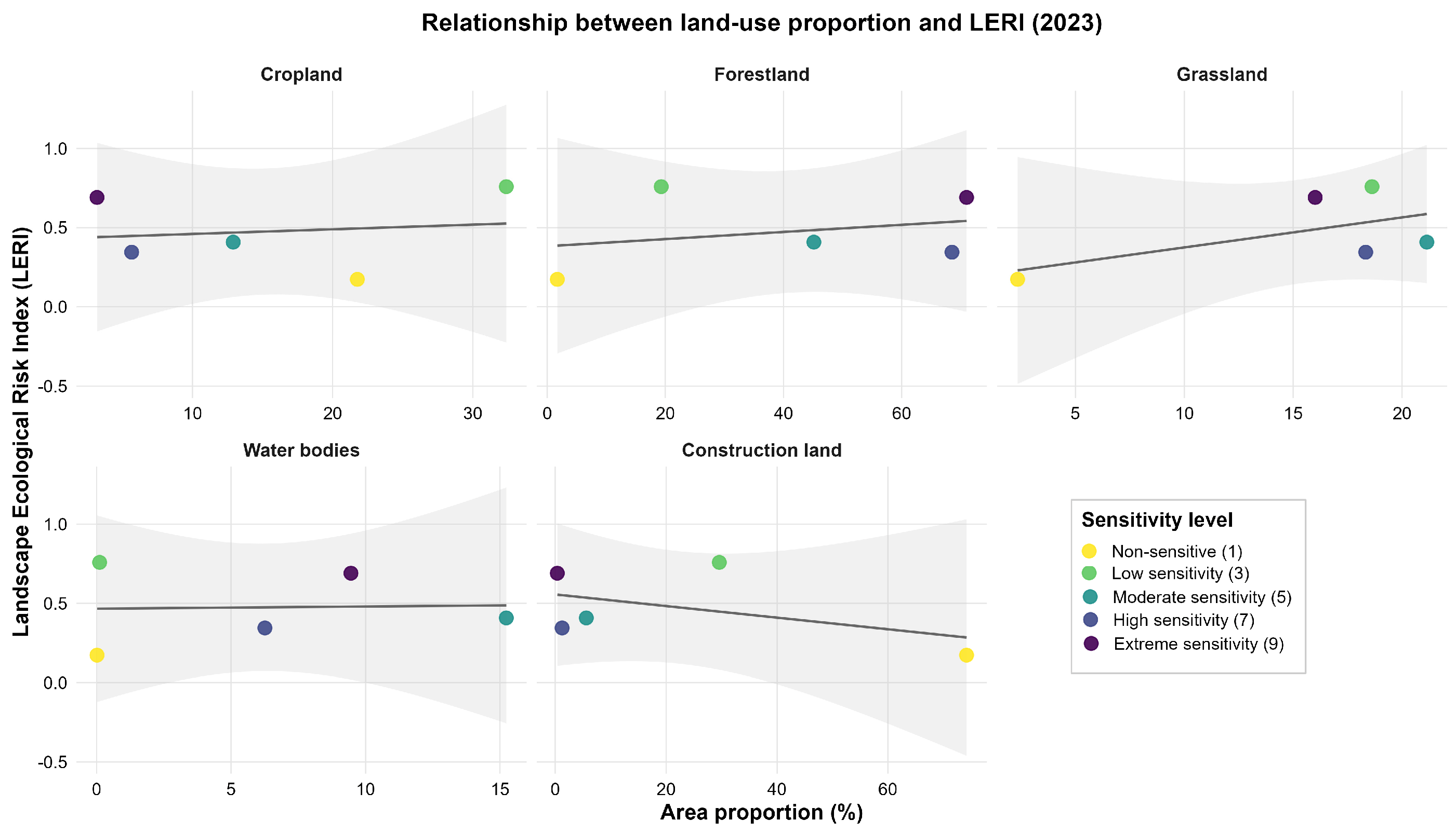
Figure 7 presents the relationships between the area proportion of each land-use type and the Landscape Ecological Risk Index (LERI) using faceted scatter plots. The grassland proportion exhibited a positive linear trend with LERI, whereas the construction land proportion showed an opposing negative trend, with higher proportions corresponding to lower LERI values. The cropland proportion displayed only a weak positive trend, while forestland and water bodies showed no discernible directional patterns. These visual patterns corroborate the explanatory factor identification results from the regression analysis: grassland and construction land are the two core land-use types driving LERI variations, exerting opposing directional effects.

3.5. Results of the Robustness Check: Land-Use Exclusion Test

To examine the potential circularity issue—where land use contributes to both the sensitivity classification and the LERI—we re-derived the ecological sensitivity zones with the land-use factor excluded and the remaining six weights re-normalized (Table S4), following the same procedure described in Section 2.3.1.

Under this alternative zonation, the low-sensitivity zone (Level 3) no longer exhibited the highest LERI—it dropped to third place (LERI = 0.4928), while the extreme-sensitivity zone (Level 9) became the highest (LERI = 0.5986; Table S5). The non-sensitive zone expanded dramatically (+121.3%; Supplementary Figure S1). This result is further interpreted in Section 4.3.

3.6. Grid-Scale Validation Results

To validate the robustness of the explanatory factors identified at the sensitivity-level scale (n = 5), we repeated the correlation and regression analyses at the grid scale using 2 km × 2 km grid cells (n = 445 valid cells after removing those with missing data). The results are summarized in Table S6.

At the grid scale, grassland showed a significant positive correlation with LERI in both Pearson (r = 0.121, p = 0.011) and Spearman (ρ = 0.147, p = 0.002) tests. Its VIP value was 1.142 (>1), with positive coefficients in both ridge regression and PLSR.

Forest (VIP = 1.387) and water (VIP = 1.118) showed negative correlations with LERI (Pearson r = −0.104, p = 0.029 and r = −0.099, p = 0.036, respectively). Cropland showed no significant correlations (r = 0.013, p = 0.789).

Construction land showed a significant Spearman correlation (ρ = 0.127, p = 0.007) but its VIP value was 0.719 (<1). The interpretation of these grid-scale results, particularly the scale-dependent behavior of construction land, is provided in Section 4.3.

4. Discussion

4.1. Mechanisms Underlying the Elevated Risk in Low-Sensitivity Zones

The core finding of this study is that the low-sensitivity zone (Level 3) exhibited the highest Landscape Ecological Risk Index (LERI = 0.7588), while the non-sensitive zone (Level 1) recorded the lowest (LERI = 0.1732). The elevated risk in the low-sensitivity zone appears to be associated not simply with the absolute extent of construction land, but rather with the landscape fragmentation induced by the mixed cropland–grassland–construction land mosaic. In this context, construction land may act as a catalyst—even without dominating the landscape, its embedment within the cropland–grassland matrix can initiate fragmentation by dissecting existing patches and increasing edge density.

From the perspective of land-use composition, the low-sensitivity zone exhibited a highly mixed composition of cropland (32.53%), grassland (18.73%), and construction land (29.55%), whereas the non-sensitive zone was dominated by construction land (74.34%), and the high-sensitivity (Level 7) and extreme-sensitivity (Level 9) zones were dominated by forestland (>68%). These compositional differences are also reflected in the landscape pattern indices: the low-sensitivity zone recorded the highest values of Number of Patches (NP) and Edge Density (ED) among the five levels, while Patch Density (PD) was also at an extremely high level (46.06), only slightly lower than that of the extreme-sensitivity zone (46.21). In contrast, the Contagion Index (CONTAG) and Aggregation Index (AI) were the lowest. High NP and ED suggest that the landscape is dissected into numerous fine patches with intensified edge effects; low CONTAG and AI are consistent with weakened connectivity and aggregation among dominant patch types. Taken together, these structural indices are consistent with a pattern of landscape fragmentation—a factor that appears to be associated with elevated ecological risk.

Ridge regression and PLSR consistently identified grassland as the strongest positive explanatory factor and construction land as the primary negative explanatory factor, supporting the interpretation that the mixed mosaic of grassland and cropland is associated with fragmentation, whereas the homogenized structure dominated by construction land corresponds to lower risk. This finding is consistent with the land-use spatial configuration across sensitivity levels. The high ridge coefficient of cropland, which dropped substantially in the PLSR, is likely attributable to collinearity. Water bodies showed no explanatory contribution.

From the perspective of temporal land-use transitions, construction land experienced a cumulative net increase of 4.68 × 10⁴ ha (+153.3%) between 2000 and 2023, coinciding with the continuous conversion of cropland and grassland. The crux lies in the locational selection of this expansion—new construction land was concentrated in flat, low-cost areas with lower ecological sensitivity, which precisely corresponds to the low-sensitivity zone (Level 3) delineated in this study. This spatial reallocation was followed by continuous cropland loss, grassland dissection, and further isolation of forestland patches, resulting in a highly mixed cropland–grassland–construction land mosaic. Landscape pattern metrics reflected this phenomenon: this intensive spatial reallocation was associated with a marked spatial reconfiguration of the landscape, manifested as the multi-indicator polarization of accelerated patch split, heightened edge dissection, and compressed structural connectivity as evidenced in Table 5. In other words, land-use transitions did not directly inflate the LERI; rather, they appear to have contributed to elevated ecological risk through reconfiguring the landscape structure—specifically by increasing the number of patches, intensifying edge effects, and weakening structural connectivity. Among the three periods, the 2010–2020 interval witnessed the most drastic changes (construction land +71.3%, cropland −18.4%, and grassland −9.4%), overlapping with the accelerated urbanization phase of Kunming City. This temporal alignment with the highest risk level ultimately observed in the low-sensitivity zone is consistent with the interpretation that historical land-use transition processes have contributed to the current risk pattern. This mechanism is particularly pronounced in the circum-Dianchi Lake region, where topographical constraints of the ecologically fragile plateau lake basin tend to concentrate developable land in flat areas. Because these areas are precisely classified as the low-sensitivity zone, they became a focal point of competition for urban and rural construction land, meaning that this zone not only absorbs most of the urban expansion but also bears the fragmentation costs generated by continuous cropland and grassland conversion. These characteristics of topographically constrained areas help explain the counterintuitive high-risk profile of the low-sensitivity zone.

4.2. Comparison with Existing Studies

Traditional ecological sensitivity assessments tend to prioritize high-sensitivity zones as the primary targets of regulatory control, while implicitly assuming that low-sensitivity zones carry lower risk and are suitable for moderate development. In contrast, the present study reveals that low-sensitivity zones, owing to landscape fragmentation induced by intensive human activities, paradoxically exhibit the highest landscape ecological risk. This counterintuitive phenomenon is not an isolated case. Jiang et al. (2025) demonstrated in the Yan River watershed that Number of Patches (NP) and Edge Density (ED) are positively correlated with landscape ecological risk—that is, landscape fragmentation directly elevates ecological risk [33]. A similar spatial mismatch of “relatively low ecological sensitivity but relatively high landscape fragmentation” has been observed in areas surrounding the Giant Panda National Park [34]. Research on the urban fringe of Xi’an further indicates that over half of the fringe area is at medium-to-high risk levels, with landscape fragmentation identified as the primary risk explanatory factor in this region [35]. Studies on the Nanjing urban–rural ecotone have confirmed that the continuous evolution of the urban–rural interface exacerbates landscape fragmentation and the intertwining of artificial and natural land-cover types [36]. Similarly, Gu et al. [37] demonstrated in the mountainous region of Heishui County, southwest China, that landscape pattern changes significantly contribute to ecological vulnerability, further corroborating the positive association between landscape dynamics and ecological risk across different geographical settings. For the Dianchi Lake Basin specifically, a terrain-gradient analysis of landscape ecological risk using the geo-information Tupu method has documented the same grassland/cropland-to-construction land conversion that underpins the fragmentation process in our study area [38]. Collectively, these studies across different regions support the view that landscape fragmentation is associated with elevated ecological risk. The coupling between urbanization and ecological security has been theorized as either coordinated or unbalanced [39], providing a conceptual framework for understanding why low-sensitivity zones—where urbanization pressure is high but regulatory protection is low—may become hotspots of ecological risk. Building upon this foundation, the present study further adopts ecological sensitivity levels as independent analytical units to quantitatively stratify fragmentation-related risk, thereby advancing the qualitative consensus that fragmentation is linked to risk toward a quantitative identification of which sensitivity level is most severely affected and which land-use type plays a primary role in the process.

At the methodological level, the innovations of this study are threefold. First, a stratified analysis was conducted using the five sensitivity levels as independent analytical units, quantifying a 4.38-fold difference in risk between the low-sensitivity and non-sensitive zones (LERI: 0.7588 vs. 0.1732), thereby providing clear spatial targets for identifying priority areas for risk regulation. Second, ridge regression (λ = 0.1) and partial least squares regression (PLSR) were jointly employed for cross-validation, which provided directionally consistent identification of explanatory factors under conditions of high multicollinearity (a strong negative correlation between cropland and construction land proportions) and a limited sample size (n = 5), thereby supporting the robustness of the conclusions. Third, an integrated mechanistic pathway was constructed from two dimensions, land-use composition and landscape pattern indices: “cropland–grassland–construction land mixed mosaic → high patch density and high edge density → landscape fragmentation → high ecological risk,” offering a clear quantitative basis for ecological risk regulation in the low-sensitivity zone.

Notably, existing studies have largely approached ecological risk assessment from the perspective of natural vulnerability, prioritizing high-sensitivity zones for risk regulation. The present study complements this perspective by offering a view from the low-sensitivity zone: under rapid urbanization, land-use-related landscape fragmentation within these zones may represent an underestimated and relatively independent source of ecological risk.

4.3. Methodological Contributions and Limitations

In the construction of the Landscape Ecological Risk Index (LERI), this study employed the entropy weight method for objective weighting, allowing the weights of each landscape pattern index to reflect their actual variability across sensitivity levels and reducing reliance on purely subjective evaluation. At the analytical framework level, the proposed “dual-coupling” approach—coupling land-use composition with ecological sensitivity, and landscape pattern with ecological sensitivity—provides a novel analytical perspective for integrated ecological risk assessments that combine natural substrates and anthropogenic disturbances in plateau lake-basin regions. This framework links land-use composition, landscape configuration, and risk response into a quantifiable chain of evidence, offering a coherent logical thread for elucidating how landscape fragmentation elevates ecological risk within low-sensitivity zones. Furthermore, for explanatory factor identification, ridge regression and partial least squares regression (PLSR) were jointly applied for cross-validation. This dual-model approach yielded directionally consistent results even under conditions of high collinearity among independent variables, strengthening the credibility of the factor identification.

To further validate the robustness of the analytical framework, two complementary robustness checks were conducted. First, to address potential circularity—where land use contributes to both the sensitivity classification and the LERI—we excluded the land-use factor from the sensitivity zoning and re-normalized the remaining six weights. Under this alternative zonation, the low-sensitivity zone (Level 3) dropped to third place in LERI ranking (0.4928), while the extreme-sensitivity zone (Level 9) became the highest (0.5986). The non-sensitive zone expanded dramatically (+121.3%), and the low-sensitivity zone no longer corresponded to the peri-urban mixed mosaic where fragmentation risk is concentrated. This result does not invalidate the core finding; rather, it demonstrates that land-use is essential for detecting human-driven fragmentation risk. When excluded, the sensitivity zoning reverts to a purely natural-substrate logic, and the anthropogenic signal is obscured. The fact that the counterintuitive pattern only emerges when land-use is included is not evidence of circularity, but confirmation that the pattern is a product of the coupled natural–human system—precisely the limitation of traditional assessments that this study addresses.

Second, to address the limited sample size at the sensitivity-level scale (n = 5), we conducted a grid-scale validation using 2 km × 2 km grid cells (n = 445). The grid-scale results confirmed that grassland remained significantly positively associated with LERI (Pearson r = 0.121, p = 0.011; VIP = 1.142 > 1), corroborating the directional consistency of the sensitivity-level findings. Forest and water showed consistently negative associations (VIP = 1.387 and 1.118, respectively). In contrast, construction land exhibited a scale-dependent pattern: its Spearman correlation was significant (ρ = 0.127, p = 0.007), but its VIP fell below one (0.719). This suggests that construction land’s effect is more strongly expressed at the sensitivity-level scale—where the contrast between the non-sensitive zone (74.34% construction land) and the low-sensitivity zone (29.55%) is most pronounced—than at the grid scale, where the effect is diluted by within-level spatial variation. This scale-dependent behavior highlights the value of stratified analysis in capturing structural contrasts that may be masked by within-level heterogeneity.

Notably, metrics such as PLADJ and AI tend to decrease as land-use mixing increases, which may raise the question of whether the elevated LERI in the low-sensitivity zone partly reflects the index construction itself rather than an independent empirical finding. In response, we argue that the low-sensitivity zone simultaneously exhibits extreme values in both positive indicators (NP, PD, ED, and IJI) and negative indicators (CONTAG, PLADJ, and AI)—ranking highest or second-highest in the former and lowest in the latter. This systematic polarization is unlikely to be explained by the mathematical properties of individual metrics; rather, it reflects a genuine spatial condition of intense landscape fragmentation and high interspersion among different patch types. Therefore, the systematic differentiation of sensitivity levels by LERI—with the low-sensitivity zone ranking highest and the non-sensitive zone lowest—is grounded in genuine landscape heterogeneity.

This study also has several limitations. First, the determination of weights in the ecological sensitivity evaluation using the Analytic Hierarchy Process (AHP) relies on expert experience, meaning subjective components cannot be entirely eliminated. Second, the explanatory factor analysis was initially conducted using the five ecological sensitivity levels as statistical units, yielding a limited sample size (n = 5) that constrains statistical power at this scale. At the sensitivity-level scale, although the Pearson and Spearman correlation coefficients exhibited consistent directional patterns, none reached conventional significance levels. To address this limitation, we conducted a grid-scale validation (n = 445), which confirmed that grassland remained significantly correlated with LERI (p < 0.05). Nevertheless, the stability of the coefficient estimates at the sensitivity-level scale requires further validation with larger samples. Third, the LERI and landscape pattern indices were calculated using 2023 as the baseline year. While this provides a consistent spatial stratification framework for evaluating land-use-driven risk, it does not capture the full temporal trajectory of risk evolution. Future research incorporating multi-temporal LERI calculations would strengthen the understanding of risk dynamics over time. Fourth, while the use of ecological sensitivity levels as the analytical scale facilitates the identification of systematic differences among levels, it inevitably masks within-level heterogeneity. Furthermore, the current mechanistic interpretation relies primarily on landscape pattern indices and lacks direct observational data on ecological processes, such as soil and hydrological dynamics. These constraints may be progressively addressed in future research by incorporating finer analytical scales, multi-temporal remote sensing data, and field monitoring, thereby facilitating the development of more robust risk assessment models.

4.4. Implications for Ecological Risk Assessment and Landscape Management

The “mixed mosaic → fragmentation → high risk” mechanism revealed in this study provides directional support for differentiated landscape management. For the fragmentation-driven high-risk phenomenon within the low-sensitivity zone, landscape regulation in this area should focus on reducing patch fragmentation and enhancing landscape connectivity. Specific pathways may include cropland-to-grassland conversion, integration of scattered patches, and ecological corridor construction, aiming to simultaneously reduce the Number of Patches (NP) and Edge Density (ED) while increasing the Contagion Index (CONTAG). In the construction-land-dominated non-sensitive zone, the association between homogenized landscape structure and low risk suggests that maintaining a concentrated and contiguous construction pattern and curbing the disorderly sprawl of construction land into low-sensitivity zones are key spatial regulation directions for preventing the diffusion of fragmentation. For the high-sensitivity and extreme-sensitivity zones, the spatial integrity of contiguous forestland constitutes the core foundation for maintaining landscape function. Priority should be given to protecting forest patches with high connectivity, avoiding dissection by linear infrastructure, and progressively restoring damaged connection areas through enclosure measures.

To further support the above zonal regulation pathways, it is recommended that key landscape pattern metrics be incorporated into the monitoring and early warning system for regional ecological risk assessment. Indices that contribute significantly to LERI—such as NP, ED, CONTAG, and COHESION—can serve as quantitative early warning signals of fragmentation risk, enabling the identification of patches within each sensitivity level where fragmentation is occurring or may be intensifying. Coupled with multi-temporal landscape pattern dynamic monitoring (e.g., updated every five years), this approach is expected to establish a tiered response framework of “risk level–regulation intensity,” providing a scientific basis for coordinating regional ecological security and sustainable land use at the spatial planning level.

5. Conclusions

This study constructed a dual-coupling analytical framework integrating (i) land-use composition with ecological sensitivity and (ii) landscape pattern with ecological sensitivity and validated it using the urban construction area around Dianchi Lake in Kunming City as a case study. The findings revealed that landscape ecological risk did not increase monotonically with ecological sensitivity levels, but rather peaked in the low-sensitivity zone (LERI = 0.7588). This counterintuitive pattern stemmed from landscape fragmentation induced by the mixed mosaic of cropland, grassland, and construction land within the low-sensitivity zone—grassland was identified as the primary positive explanatory factor of LERI, while construction land served as the primary negative explanatory factor.

Grid-scale validation, however, revealed a more complex pattern: grassland was the only factor whose direction and importance replicated consistently across both scales (grid-scale VIP = 1.142, p = 0.002), whereas construction land showed a sign reversal with VIP falling below the threshold (VIP = 0.719), and forest shifted from negligible at the sensitivity-level scale to a significant negative predictor at the grid scale (VIP = 1.387).

Furthermore, the low-sensitivity, high-risk ranking was conditional on including land-use in the sensitivity zoning—when excluded, the low-sensitivity zone dropped to third place (0.7588 → 0.4928) and the extreme-sensitivity zone became the highest (0.6906 → 0.5986). This confirms that the decoupling between sensitivity and risk is a product of the coupled natural–human system, not a fixed landscape property, and highlights the value of the dual-coupling framework in capturing anthropogenic fragmentation signals that purely natural-factor assessments miss.

In contrast, the non-sensitive zone, dominated by contiguous construction land, exhibited a homogenized landscape structure and the lowest risk. These findings suggest that ecological risk assessment should not delineate protection areas based solely on natural sensitivity, but should also incorporate landscape pattern risks arising from land-use structure. In the low-sensitivity zone, landscape regulation measures aimed at reducing patch fragmentation and enhancing landscape connectivity can help mitigate fragmentation-driven ecological risk. The dual-coupling framework developed in this study provides a transferable methodological pathway for integrated ecological risk assessment in plateau lake-basin regions.

References

1. Chen, X.; Zhang, H.; Wong, C.U.I.; Li, F. Ecological Sensitivity Assessment of Central Plains Cities Using RS/GIS Technology: A Case Study of the Zheng-Bian-Luo Urban Agglomeration. Pol. J. Environ. Stud. 2025, 34, 4633–4645. [Google Scholar] [CrossRef] [Scilit]
2. Wang, J.; Song, Y.; Ge, B.; Zhou, Y. Dynamic Spatiotemporal Land Use Evolution in China‘s Plateau Lake Basins in Response to Landscape Ecological Sensitivity. Sustainability 2023, 15, 15020. [Google Scholar] [CrossRef] [Scilit]
3. Zhang, Q.; Wang, G.; Yuan, R.; Singh, V.P.; Wu, W.; Wang, D. Dynamic Responses of Ecological Vulnerability to Land Cover Shifts over the Yellow River Basin, China. Ecol. Indic. 2022, 144, 109554. [Google Scholar] [CrossRef] [Scilit]
4. Chen, H.; Ren, J.; Ren, W.; Luan, H.; Luo, L. Land Use Change Patterns and Landscape Ecological Risk Assessment in the Process of Watershed Ecological Compensation. Front. Environ. Sci. 2025, 13, 1723453. [Google Scholar] [CrossRef] [Scilit]
5. Deng, G.; Jiang, H.; Zhu, S.; Wen, Y.; He, C.; Wang, X.; Sheng, L.; Guo, Y.; Cao, Y. Projecting the Response of Ecological Risk to Land Use/Land Cover Change in Ecologically Fragile Regions. Sci. Total Environ. 2024, 914, 169908. [Google Scholar] [CrossRef] [Scilit]
6. Zhang, X.; Song, W. From Static to Predictive Indicators: Construction of China’s Spatiotemporal Risk Zoning Index for Land Use Changes Ecological Risks. Ecol. Indic. 2025, 179, 114154. [Google Scholar] [CrossRef] [Scilit]
7. Liu, Y.; Zhang, Y. Responses of Ecosystem Services to Land Use/Cover Changes in Rapidly Urbanizing Areas: A Case Study of the Shandong Peninsula Urban Agglomeration. Sustainability 2024, 16, 6100. [Google Scholar] [CrossRef] [Scilit]
8. Feng, R.; Wang, F.; Wang, K. Urban–Rural Differences in Cropland Loss and Fragmentation Caused by Construction Land Expansion in Developed Coastal Regions: Evidence from Jiangsu Province, China. Remote Sens. 2025, 17, 2470. [Google Scholar] [CrossRef] [Scilit]
9. Yang, F.; Yang, L.; Fang, Q.; Yao, X. Impact of Landscape Pattern on Habitat Quality in the Yangtze River Economic Belt from 2000 to 2030. Ecol. Indic. 2024, 166, 112480. [Google Scholar] [CrossRef] [Scilit]
10. Che, M.; Yang, F.; Sun, J.; Zhang, C.; Zhang, J. Influence of Road Network Expansion on the Landscape Ecological Risk in the Yangtze River Delta Region over the Past Two Decades. Ecol. Indic. 2023, 156, 111178. [Google Scholar] [CrossRef] [Scilit]
11. Qiu, M.; Liu, D. Assessing Spatial Heterogeneous Response of Ecosystem Service Relationships to Land Use Intensification. Ecol. Indic. 2023, 154, 110721. [Google Scholar] [CrossRef] [Scilit]
12. Wang, Y.; Yang, X.; Zhang, X.; Zhu, L.; Wang, X.; Li, Y.; Zhou, L.; Yu, X. Spatiotemporal Dynamic Characteristics and Conservation Strategy of Ecological Security Pattern in a Rapidly Urbanizing Zone. Ecol. Indic. 2024, 166, 112457. [Google Scholar] [CrossRef] [Scilit]
13. Wang, S.; Xu, Q.; Yi, J.; Wang, Q.; Ren, Q.; Li, Y.; Gao, Z.; Li, Y.; Wu, H. An Ecological Risk Assessment of the Dianchi Basin Based on Multi-Scenario Land Use Change Under the Constraint of an Ecological Defense Zone. Land 2025, 14, 868. [Google Scholar] [CrossRef] [Scilit]
14. Chayakul, J.; Veldwisch, G.J.; Bruins, B.; Boelens, R. Contested Waters: Hydrosocial Territories and Power Dynamics in the Landscape of Peri-Urban Chiang Mai, Thailand. Geoforum 2026, 169, 104457. [Google Scholar] [CrossRef] [Scilit]
15. Nong, D.H.; Fox, J.M.; Saksena, S.; Lepczyk, C.A. The Use of Spatial Metrics and Population Data in Mapping the Rural-Urban Transition and Exploring Models of Urban Growth in Hanoi, Vietnam. Environ. Urban. ASIA 2021, 12, 156–168. [Google Scholar] [CrossRef] [Scilit]
16. European Environment Agency. Urban Sprawl in Europe: The Ignored Challenge; EEA Report No. 10/2006; European Environment Agency: Copenhagen, Denmark, 2006. Available online: https://www.eea.europa.eu/publications/eea_report_2006_10 (accessed on 1 July 2026).
17. European Environment Agency. Landscape Fragmentation in Europe; EEA Report No. 2/2011; European Environment Agency: Copenhagen, Denmark, 2011. Available online: https://www.eea.europa.eu/publications/landscape-fragmentation-in-europe (accessed on 15 June 2026).
18. Biasi, R.; Brunori, E.; Serra, P.; Perini, L.; Salvati, L. Towards Resilient Agro-Forest Systems in Mediterranean Cities. Acta Hortic. 2017, 1189, 125–130. [Google Scholar] [CrossRef] [Scilit]
19. Lin, M.; Chen, Y.; Zhang, J.; Lin, T.; Liu, Y.; Geng, H.; Jia, Z. Scale and Zoning Effects on Landscape Metrics for Assessing Ecological Stress from Urban Expansion. Landsc. Ecol. 2024, 39, 211. [Google Scholar] [CrossRef] [Scilit]
20. Wang, H.; Hua, M.; Wang, S.; Niu, J.; Wang, Y.; Li, X. An Improved Framework for Assessing Territorial Spatial Conflict from the Perspective of Ecological Security and Its Quantitative Analysis of Driving Factors: A Case Study of the Yellow River Basin. Environ. Prog. Sustain. Energy 2026. early view. [Google Scholar] [CrossRef] [Scilit]
21. Huang, B.; Yang, H.; Shang, K.; Wang, R.; Meng, Y.; Peng, H.; Hu, Y.; Jiang, Z. A SDGs-Oriented Evaluation of the Ecological Sustainability of International Horticultural Exposition Sites in Chengdu, China. J. Environ. Eng. Landsc. Manag. 2025, 33, 118–131. [Google Scholar] [CrossRef] [Scilit]
22. Amporn, P.; Choemprayong, S.; Srichaichana, J. Spatial Ecological Risk Assessment of Kaeng Krachan National Park, Thailand (UNESCO World Heritage Site) through Integration of AHP, Shannon’s Entropy, and Monte Carlo Simulation. Model. Earth Syst. Environ. 2026, 12, 10. [Google Scholar] [CrossRef] [Scilit]
23. Ma, D.; Huang, Q.; Zhang, Q.; Wang, Q.; Xu, H.; Yan, Y. Evaluation of Eco-Environmental Quality and Analysis of Driving Forces in the Yellow River Delta Based on Improved Remote Sensing Ecological Indices. Stoch. Environ. Res. Risk Assess. 2024, 38, 3199–3220. [Google Scholar] [CrossRef] [Scilit]
24. Tuljak-Suban, D.; Suban, V. Ecological Risk Assessment of the Adriatic Coastline: An Environmental Sensitivity Index Developed Through Expert Surveys and the Entropy Weight Method. Clean—Soil Air Water 2025, 53, 70077. [Google Scholar] [CrossRef] [Scilit]
25. Lisiak-Zielińska, M.; Borowiak, K.; Budka, A.; Cakaj, A.; Hanć, A.; Wiatrowska, K. Rare Earth Elements and Landscape: Is There a Relationship between Them?—New Evidence from Poland (Eastern Europe). Ecol. Indic. 2024, 159, 111642. [Google Scholar] [CrossRef] [Scilit]
26. Nyirarwasa, A.; Han, F.; Yang, Z.; Mperejekumana, P.; Umwali, E.D.; Nsengiyumva, J.N.; Habibulloev, S. Evaluating the Impact of Environmental Performance and Socioeconomic and Demographic Factors on Land Use and Land Cover Changes in Kibira National Park, Burundi. Sustainability 2024, 16, 473. [Google Scholar] [CrossRef] [Scilit]
27. Li, C.; Qin, F.; Liu, Z.; Pan, Z.; Gao, D.; Han, Z. Multi-Scenario Assessment of Landscape Ecological Risk in the Transitional Zone between the Warm Temperate Zone and the Northern Subtropical Zone. Front. Ecol. Evol. 2025, 12, 1471164. [Google Scholar] [CrossRef] [Scilit]
28. Tankpa, V.; Wang, L.; Awotwi, A.; Singh, L.; Thapa, S.; Atanga, R.A.; Guo, X. Modeling the Effects of Historical and Future Land Use/Land Cover Change Dynamics on the Hydrological Response of Ashi Watershed, Northeastern China. Environ. Dev. Sustain. 2021, 23, 7883–7912. [Google Scholar] [CrossRef] [Scilit]
29. Durango-Cordero, J.; Saqalli, M.; Bonilla, S.F.; Elger, A. Vulnerability Assessment of Natural Heritage in the North-Eastern Ecuadorian Amazon Using Land Use Cover and Nature Protection Status. J. Nat. Conserv. 2024, 81, 126686. [Google Scholar] [CrossRef] [Scilit]
30. Li, Z.; Xu, X.; Zhu, J.; Xu, C.; Wang, K. Sediment Yield Is Closely Related to Lithology and Landscape Properties in Heterogeneous Karst Watersheds. J. Hydrol. 2019, 568, 437–446. [Google Scholar] [CrossRef] [Scilit]
31. Mahieu, B.; Qannari, E.M.; Jaillais, B. Extension and Significance Testing of Variable Importance in Projection (VIP) Indices in Partial Least Squares Regression and Principal Components Analysis. Chemom. Intell. Lab. Syst. 2023, 242, 104986. [Google Scholar] [CrossRef] [Scilit]
32. Wold, S.; Sjöström, M.; Eriksson, L. PLS-Regression: A Basic Tool of Chemometrics. Chemom. Intell. Lab. Syst. 2001, 58, 109–130. [Google Scholar] [CrossRef] [Scilit]
33. Jiang, X.; Jiang, Z.Y.; Li, Z.Y.; Su, J.; Tang, L.N.; Wu, M.D.; Wang, Y.J. A Framework for the Construction of Effective Landscape Ecological Network with Integrating Hydrological Connectivity: A Case Study in Dongjiang River Basin, China. J. Environ. Manag. 2025, 376, 124509. [Google Scholar] [CrossRef] [Scilit]
34. Xia, H.; Lu, F.; Li, J. Spatial Correlation of Landscape Fragmentation and Ecological Sensitivity in China’s Giant Panda National Park and Surrounding Areas. Sustainability 2024, 16, 7371. [Google Scholar] [CrossRef] [Scilit]
35. Wu, W.; Zhou, L.; Wang, S.; Wei, W.; Chen, Z.; Zhang, Q.; Wang, W. Identification of Urban Fringe Areas and Assessment of Their Landscape Ecological Risks in Xi’an, China. Chin. Geogr. Sci. 2025, 35, 1013–1029. [Google Scholar] [CrossRef] [Scilit]
36. Cao, H.; Li, P.; Chen, J.; Chen, C.; Song, W. Spatiotemporal Evolution of the Rural-Urban Interface and Its Effects on Ecological Landscape Structure and Function: A Case Study of Nanjing, China. Ecol. Indic. 2024, 166, 112267. [Google Scholar] [CrossRef] [Scilit]
37. Gu, W.; Fu, H.; Jin, W. Landscape Pattern Changes and Ecological Vulnerability Assessment in Mountainous Regions: A Multi-Scale Analysis of Heishui County, Southwest China. Land 2025, 14, 314. [Google Scholar] [CrossRef] [Scilit]
38. Wang, Q.; Yang, K.; Li, L.; Zhu, Y. Assessing the Terrain Gradient Effect of Landscape Ecological Risk in the Dianchi Lake Basin of China Using Geo-Information Tupu Method. Int. J. Environ. Res. Public Health 2022, 19, 9634. [Google Scholar] [CrossRef] [Scilit]
39. Shi, Y.; Feng, C.-C.; Yu, Q.; Han, R.; Guo, L. Contradiction or Coordination? The Spatiotemporal Relationship between Landscape Ecological Risks and Urbanization from Coupling Perspectives in China. J. Clean. Prod. 2022, 363, 132557. [Google Scholar] [CrossRef] [Scilit]
Figure 1. Urban built-up area around Dianchi Lake, Kunming.
Land 15 01567 g001
Figure 2. The methodological framework of this study.
Land 15 01567 g002
Figure 3. Land-use distribution and sensitive-area zoning in 2023.
Land 15 01567 g003
Figure 4. Land-use composition across ecological sensitivity levels in 2023. Values within each category denote the area proportion (%) and the corresponding area (×104 ha).
Land 15 01567 g004
Figure 5. Variations in ecological risk and landscape pattern across the ecological sensitivity gradient. (a) LERI values for each sensitivity level. (b,c) Radar charts of positive and negative indicators. The radar charts reveal that the low-sensitivity zone expands outward on positive indicators and contracts inward on negative indicators, reflecting its fragmentation signature.
Land 15 01567 g005
Figure 6. Land-use area changes across three periods (2000–2023).
Land 15 01567 g006
Figure 7. Relationships between the proportions of the five land-use types and the Landscape Ecological Risk Index (LERI).
Land 15 01567 g007