Coupling Trend–Pattern Dynamics for Synergistic Governance: A Multi-Scale Assessment of Carbon Emissions and Ecosystem Services in the Yellow River Basin

Abstract

Achieving synergistic governance between carbon emissions and ecosystem service value (ESV) in the Yellow River Basin (YRB) remains a significant challenge. Existing studies often rely on a single administrative scale and rarely extend spatial clustering results toward governance-oriented zoning frameworks that support differentiated management. To bridge these gaps, we developed a multi-scale remote sensing framework by integrating the China Land Cover Dataset (CLCD), NPP/VIIRS nighttime light (NTL) imagery, and energy consumption statistics to examine carbon emissions and ESV across the YRB at both county and grid scales. We estimated land-use carbon emissions by integrating emission coefficients with NTL modeling, while ESV was quantified via the equivalent factor method. By coupling dynamic carbon–ESV trends with their spatial association patterns (derived from bivariate LISA), we established a dual-dimensional Trend–Pattern framework for synergistic governance. Our findings reveal a pronounced asymmetry in regional development: while carbon emissions surged from 235 to 1033 million tons, ESV grew by a marginal 0.13% annually. Although carbon emissions and ESV are significantly negatively correlated (p < 0.001), this relationship diverges across scales—weakening at the county level but intensifying at the grid level. Notably, grid-scale analysis identified a contraction of over 56% in “Low carbon–High ESV” synergistic clusters in the upper reaches. This critical signal of declining carbon–ecological synergy was completely obscured by the averaging effect inherent in county-level assessments. Capitalizing on these scale-dependent insights, we delineated seven distinct governance zones, including Trend Control and Ecological Conservation Zones, thereby transitioning from mere spatial description to decision support for zoning-based governance. This study highlights the potential limitations of relying solely on single-tier administrative evaluations and offers a robust, multi-scale decision-support tool for carbon–ecological governance in the YRB.

1. Introduction

With the intensification of global climate warming and the continuous advancement of carbon neutrality agendas, the coordinated and sustainable development of the “carbon–ecology–economy” system has become a central research topic worldwide [1,2,3]. The Yellow River Basin (YRB), as an important ecological security barrier, energy supply corridor, and grain production base in China, has substantial carbon emissions, accounting for 33.11% of China’s total carbon emissions [4,5,6]. Meanwhile, the YRB provides irreplaceable ecosystem services, including water conservation, soil and water conservation, biodiversity maintenance, and climate regulation [7,8]. In recent years, rapid economic development in the YRB has been accompanied by substantial changes in land use. The unregulated expansion of urban construction land and the conversion among different land-use types have led to significant regional differences in carbon emissions [9,10]. At the same time, changes in land cover have also exerted important impacts on ecosystem service value (ESV). Functional differences among land-use types, together with the direct and indirect changes in total carbon emissions and ESV caused by land-use transitions, have therefore become important research topics [11,12].

From the perspective of sustainability science, the relationship between land-use carbon emissions and ecosystem services can be interpreted through the pressure–state–response (PSR) model [13,14,15]. Land-use conversion, urban expansion, and energy–intensive socioeconomic activities generate carbon emissions and therefore constitute major anthropogenic pressures on regional social–ecological systems. ESV reflects the ecological state and functional capacity of ecosystems to provide provisioning, regulating, supporting, and cultural services. In turn, differentiated emission-reduction, ecological conservation, and restoration measures represent societal responses to observed pressure–state mismatches. Within this theoretical logic, the temporal trends of carbon emissions and ESV indicate whether the pressure–state relationship is improving, remaining stable, or deteriorating, whereas their spatial association patterns reveal where synergistic or conflicting relationships are concentrated. Coupling temporal trends with spatial patterns therefore operationalizes the PSR model across both temporal and spatial dimensions and provides a theoretical basis for translating diagnostic assessment into place-specific governance responses.

Extensive research has been conducted on land-use carbon emissions worldwide, covering carbon emission accounting, the spatiotemporal evolution and influencing factors of total carbon emissions or emission intensity, carbon emission prediction, zoning-based carbon emission management, and the decoupling relationship between carbon emissions and economic growth [16,17,18,19,20]. These studies have been conducted at multiple scales, including national, basin, provincial, prefecture-level city, and county scales. Research on the impact of land-use change on ESV has mainly focused on the spatiotemporal evolution of ESV, scenario simulation and future prediction, and driving mechanisms [21,22,23]. As the core carrier of carbon–ecological interactions, land use directly drives both carbon emissions and ESV changes [24]. For example, the conversion of forests to cropland may result in CO₂ release, while wetland loss may weaken hydrological regulation functions. Accordingly, increasing attention has recently been paid to the relationship between carbon emissions and ESV. For instance, Chen et al. used spatial autocorrelation indices and LISA cluster maps to examine the county-scale relationship between land-use carbon emissions and ESV in the YRB, and further explored the factors influencing spatial correlations using a multinomial Logit regression model [25]. Wang et al. introduced variables such as carbon sources, carbon sinks, net carbon emissions, carbon emission intensity, and ESV intensity to investigate the spatiotemporal evolution of carbon emissions and ESV in the Nansi Lake Basin and analyze their spatial association [26]. Fu et al. examined the spatiotemporal coupling relationship between carbon emissions and ESV in the Poyang Lake Basin using spatial autocorrelation and Pearson correlation analysis [27]. These studies have helped fill the research gap at the intersection of carbon emissions and ecosystem services and have promoted the development of land system science. Exploring the relationship between carbon emissions and ESV is important for revealing the underlying mechanisms of land-use spatial conflicts, providing coordinated “carbon–ecology” management tools for sustainable development in the YRB, guiding ecological risk prevention, and supporting the optimization of land-use planning toward low-carbon and high-service-value land-use patterns [28].

Recent studies have examined the spatial relationship between carbon emissions and ESV within the YRB and other major watersheds using spatial autocorrelation and LISA analyses [29,30,31,32]. These studies have substantially improved the understanding of carbon–ecological interactions at regional scales. Although the body of research on land-use carbon emissions and ESV is growing, two limitations remain. First, existing studies are often restricted to a single analytical scale. Most studies have been conducted at the prefecture-level city or county scale, while only a limited number have adopted grid-based analysis [29,30]. A systematic comparison of the spatial association between carbon emissions and ESV at both county and grid scales remains insufficient. Second, although bivariate LISA has been widely used to identify spatial association patterns between carbon emissions and ecosystem services, most existing studies treat LISA primarily as a descriptive analytical tool. Few studies integrate temporal evolution trajectories with spatial association patterns to construct governance-oriented zoning frameworks capable of supporting differentiated management [31,32]. This creates a clear “translation gap” between research findings and policy practice. Therefore, studies on the coupling relationship between carbon emissions and ESV in the YRB urgently require a multi-scale and zoning-oriented analytical framework to bridge the gap between spatial pattern identification and land-use policy implementation.

To address these research gaps, this study makes two main contributions. First, it develops a multi-scale analytical framework that integrates land-cover products, nighttime light imagery, and statistical energy data to examine carbon emissions—ESV interactions at both county and grid scales. Analyses are conducted simultaneously at the county scale, representing administrative decision-making units, and at the 3 km × 3 km grid scale, representing continuous natural spatial units. Comparing these two scales enables assessment of how spatial aggregation influences the identification of carbon–ESV relationships while revealing localized heterogeneity that may be obscured by administrative averaging. Compared with previous county-level studies, the 3 km grid analysis captures localized spatial heterogeneity and reduces the masking effect caused by administrative aggregation, thereby providing a more detailed basis for identifying carbon–ecological conflicts. The selected 3 km resolution provides a balance between capturing local spatial heterogeneity and maintaining consistency with multi-source datasets [33]. Second, inspired by the PSR perspective in sustainability science, this study develops a governance-oriented analytical framework for diagnosing and managing the interactions between carbon emissions and ESV. Within this perspective, carbon emissions represent anthropogenic pressure, ESV reflects the state of ecosystem functioning and service-provision capacity, and differentiated governance zoning constitutes the societal response. Accordingly, this study proposes a Trend–Pattern framework, defined as a dual-dimensional analytical framework that integrates temporal evolution trends with spatial association patterns to characterize the coupled dynamics between carbon emissions and ESV. Unlike conventional studies that primarily use LISA to describe spatial association patterns [31,32], the proposed Trend–Pattern framework integrates temporal evolution with spatial association, enabling the use of diagnostic results to support governance zoning and differentiated management decisions.

Unlike conventional ecological zoning or conflict zoning approaches, which primarily delineate management units based on static spatial characteristics, the proposed framework explicitly incorporates the evolutionary trajectories of carbon–ESV interactions, thereby supporting adaptive and differentiated governance rather than one-time spatial classification. Specifically, the Trend dimension describes the temporal trajectories of the coupled carbon emission–ESV based on directional changes across consecutive periods, distinguishing five dynamic evolution types: improving, deteriorating, conflicting, recessive, and stable. The Pattern dimension characterizes the spatial configuration of carbon–ESV interactions identified by bivariate LISA, including High–Low (H–L), Low–High (L–H), High–High (H–H), and Low–Low (L–L) association types. By coupling these temporal and spatial dimensions, the Trend–Pattern framework translates spatiotemporal diagnosis into governance-oriented decision support, enabling differentiated zoning with explicit governance objectives and policy recommendations. Overall, this study advances the research from “pattern description” to “zoning governance” and expands both the analytical framework and research perspective, providing spatial decision support for the coordinated promotion of ecological protection and high-quality development in the YRB.

Accordingly, this study addresses the following research questions:

(1)

How have carbon emissions and ESV evolved across county and grid scales in the YRB during 2000–2020?

(2)

How do the spatial associations between carbon emissions and ESV differ across spatial scales?

(3)

Can the proposed Trend–Pattern framework translate multi-scale spatiotemporal diagnosis into differentiated governance zoning?

2. Study Area and Data

2.1. Study Area

The YRB is an important ecological security barrier and economic zone in China. It spans the Qinghai–Tibet Plateau, the Loess Plateau, and the North China Plain, and is characterized by complex and diverse topographic conditions. The basin also contains national-level urban agglomerations, such as the Central Plains Urban Agglomeration, as well as energy resource-rich areas in Shanxi, Shaanxi, Inner Mongolia, and Ningxia. Under the combined influence of natural endowments and human activities, land-use patterns in the basin have undergone frequent spatiotemporal changes. The spatial mismatch and interactions between land-use-driven carbon emissions and ecosystem services make the YRB a representative region for investigating their coordinated development. In this study, the research area was defined based on the natural boundary of the YRB. Using the basin boundary data released by the National Earth System Science Data Center [34], all county-level administrative units intersecting the YRB were identified. To maintain the integrity of administrative units and ensure consistency with county-level statistical data, these counties were retained as complete administrative entities rather than being clipped by the basin boundary. As a result, 452 county-level administrative units across nine provinces and autonomous regions were selected as the research objects. The location of the study area is shown in Figure 1.

2.2. Data Sources

The data used in this study mainly include the following four types (shown in

Table 1. Datasets and sources used in this study.

Dataset	Period	Resolution	Unit	Source	Preprocessing	Application
CLCD	2000, 2010, 2020	30 m	N/A	Yang & Huang [35], Zenodo, https://doi.org/10.5281/zenodo.12779975	Reprojection; clipping; county/grid statistics	Natural land carbon emissions; ESV calculation
NPP/VIIRS-like NTL	2000–2020	500 m	nW·cm−2·sr−1	Chen et al. [36]; Harvard Dataverse, https://doi.org/10.7910/DVN/YGIVCD	Reprojection; clipping; provincial aggregation	Province-specific NTL–energy-related carbon emission regression; grid carbon emission allocation
Provincial energy consumption statistics	2000–2020	Provincial level	Physical units as Notes; Carbon emissions (104 t)	China Energy Statistical Yearbook and provincial statistical yearbooks	Standard-coal conversion; provincial energy-related carbon emissions calculation	Energy-related carbon emissions estimation; establishment and calibration of regression models.
Crop statistics	2000, 2010, 2020	Provincial level	Price: yuan t−1; yield: t ha−1; sown area: ha; total production: t	National Compilation of Cost and Benefit Data of Agricultural Products; China Statistical Yearbook	Standard ESV equivalent calculation	Standard ESV equivalent coefficient localization.

Note: The consumption units were 10⁴ t for coal, coke, crude oil, diesel oil, kerosene, gasoline, and fuel oil; 10⁸ kWh for electricity; and 10⁸ m³ for natural gas. The calculated energy-related carbon emissions were expressed in 10⁴ t.

). First, land-use data were obtained from the China Land Cover Dataset (CLCD) developed by Huang Xin’s team at Wuhan University [35]. The dataset provides annual 30 m land-cover maps from 2000 onward and includes six primary land-use categories used in this study. All datasets were projected into the Albers Equal Area projection before spatial analysis. Second, nighttime light (NTL) data were derived from the long-term NPP/VIIRS-like NTL dataset produced by Chen et al. [36], with a spatial resolution of 500 m. The dataset has been corrected for interannual inconsistency and sensor saturation using cross-sensor calibration. Annual radiance values were aggregated at the provincial level before regression analysis. Third, Yellow River Basin boundary data were obtained from the National Earth System Science Data Center [33]. To ensure temporal consistency, a unified county-level administrative boundary dataset was adopted throughout the study period. The county-level administrative units intersecting the YRB were first identified based on the natural basin boundary and retained as complete administrative units to maintain consistency with statistical data. Subsequently, a regular 3 km × 3 km grid was generated based on this unified administrative extent, and grid cells whose centroids fell within the selected county-level units were retained for grid-scale analysis. All statistical and spatial datasets were spatially matched to this unified research extent. Therefore, the county-scale and grid-scale analyses were based on the same spatial extent while using different spatial units of analysis. Fourth, provincial energy consumption statistics for coal, coke, crude oil, diesel oil, kerosene, gasoline, fuel oil, natural gas, and electricity were collected from the China Energy Statistical Yearbook and provincial statistical yearbooks for 2000–2020. All energy data were converted into standard coal equivalents using national conversion factors before carbon emission calculation.

To enable multi-scale spatial comparison while maintaining consistency among multi-source datasets, a uniform 3 km × 3 km grid was established across the YRB. The grid size was selected by considering both previous research and the characteristics of the input datasets. Previous research has demonstrated that ecosystem service assessments exhibit pronounced spatial scale effects and that spatial clustering patterns change with grid resolution, with a distinct transition occurring around the 3 km × 3 km scale [33]. Considering these findings together with the spatial resolutions of the input datasets, a 3 km grid was adopted to capture local spatial heterogeneity while effectively representing spatial clustering patterns. In addition, the selected grid is compatible with the spatial resolutions of the input datasets, allowing reliable aggregation of multi-source information. Considering the large spatial extent of the YRB, the 3 km grid also provides a practical balance between spatial detail, computational efficiency, and mitigation of the Modifiable Areal Unit Problem (MAUP).

To ensure spatial consistency across datasets with different spatial resolutions, all spatial datasets were projected into a unified Albers Equal Area coordinate system. Carbon emissions and ESV were calculated at the native spatial resolutions of the original datasets, without raster resampling. To minimize uncertainty introduced by interpolation, spatial integration was conducted through overlay analysis, spatial aggregation, and zonal statistics. The calculated results were subsequently summarized at two analytical scales: 3 km × 3 km grids and county-level administrative units.

3. Methodology

This study systematically investigates the spatiotemporal evolution, spatial association, and synergistic governance pathways of carbon emissions and ESV in the YRB from 2000 to 2020. The overall technical workflow follows a five-stage multi-scale remote sensing framework: data acquisition and preprocessing, quantitative estimation and assessment, multi-scale spatial correlation analysis, Trend–Pattern evolutionary trajectory construction, and synergistic governance zoning. First, multi-source remote sensing and statistical datasets, including CLCD land-use data, NPP/VIIRS NTL radiance data, administrative boundaries, and energy consumption statistics, were integrated. A dual-scale analytical framework was established at the county scale and 3 km grid scale. Carbon emissions from natural land were quantified using the carbon emission coefficient method, while emissions from construction land were estimated by integrating energy consumption statistics with NTL-based spatial downscaling. Model calibration and validation were conducted to improve the accuracy of the spatialized emission results.

Second, carbon emissions and ESV were quantitatively assessed for three temporal cross-sections: 2000, 2010, and 2020. ESV was estimated using a modified equivalent factor method, with localized parameters constructed based on the equivalent value table and adjusted according to regional crop characteristics. The resulting carbon emissions and ESV datasets provided dual-scale spatial base maps for subsequent analysis. Third, global and local bivariate spatial autocorrelation analyses were introduced to examine the spatial coupling relationship between carbon emissions and ESV. Global bivariate Moran’s I was used to identify the overall spatial association pattern, while local bivariate Moran’s I and Bivariate LISA clustering were applied to characterize local spatial clusters, including H–H, L–L, H–L, and L–H types. By comparing county-scale and grid-scale results, the analysis further revealed cross-scale differences, administrative homogenization effects, and localized variations in carbon–ESV spatial association patterns.

Fourth, a Trend–Pattern evolutionary trajectory framework was proposed to identify the dynamic changes in carbon emissions–ESV relationships during 2000–2010 and 2010–2020. The proposed Trend–Pattern framework consists of two complementary components: (1) Trend analysis, which captures the temporal evolution of carbon emissions and ESV through change trajectories across successive periods, and (2) Pattern analysis, which characterizes their spatial association using bivariate LISA. These two components are subsequently coupled to support governance zoning. Based on the changing directions of carbon emissions and ESV, five dynamic types were classified, namely Deteriorating, Improving, Conflicting, Recessive, and Stable. These two-stage dynamic types were further reconstructed into three temporal trajectory pathways: persistent, positive transition, and negative transition. Meanwhile, dominant spatial patterns were extracted from bivariate LISA results, including HL-dominant, LH-dominant, HH-dominant, and LL-dominant modes. Finally, temporal trajectories and spatial patterns were coupled through a cross-classification matrix to delineate differentiated governance zones. Seven governance zones were identified: Trend Control Zone, Ecological Conservation Zone, Synergistic Governance Zone, Stable Development Zone, General Governance Zone, Ecological Restoration Zone, and Core Synergistic Governance Zone. The classification matrix was developed based on the combined ecological implications of temporal evolution trends and spatial association patterns. Trend categories indicate whether carbon–ESV relationships are improving or deteriorating over time, whereas Pattern categories identify the dominant spatial interaction characteristics. Their combination reflects different governance priorities, thereby providing a logical basis for governance zoning. Accordingly, targeted governance strategies, including emission control, ecological compensation, industrial decoupling, dynamic monitoring, ecological restoration, and systemic remediation, were proposed to support coordinated low-carbon development and ecological protection in the YRB. The technical workflow is shown in Figure 2 and summarizes the overall methodological framework of this study.

3.1. Estimation of Land-Use Carbon Emissions

In this study, land-use carbon emissions in the YRB refer to the integrated carbon balance associated with different land-use types, including carbon emissions or sequestration from natural land-use types and energy-related carbon emissions from built-up land. All carbon emissions reported in this study are expressed as tonnes of carbon. For natural land-use types, including forestland, grassland, cropland, water bodies, unused land, and wetlands, carbon emissions were estimated using the carbon emission coefficient method, as shown in Equation (1). For built-up land, energy-related carbon emissions associated with human activities were estimated using a fitting model based on energy consumption data and NTL data. Total land-use carbon emissions were obtained by summing the carbon emissions or sequestration from natural land-use types and the spatialized energy-related carbon emissions from built-up land. Negative coefficients for natural ecosystems indicate carbon sequestration and therefore offset part of the positive emissions generated by built-up land. It should be clarified that the estimated land-use carbon emissions do not represent process-based carbon emissions directly caused by land-use conversion. Instead, they represent the combined effects of natural land-use carbon fluxes and spatially allocated energy-related emissions. Therefore, changes in land-use carbon emissions among 2000, 2010, and 2020 reflect variations in land-use composition and anthropogenic energy activities rather than direct emissions generated during land-use transition processes. It should also be noted that the estimated land-use carbon emissions represent an accounting-based estimate derived from land-use categories and energy-related emissions rather than a complete biogeochemical carbon balance involving all ecosystem carbon cycling processes.

$$C_k=\sum c_i=\sum s_i\times {\beta }_i,$$

(1)

where $C_k$ represents the total carbon emissions from natural land-use types (t); $c_i$ represents the carbon emissions from land-use type I (t); and $s_i$ and ${\beta }_i$ represent the area of land-use type i (ha) and its carbon emission coefficient (t/ha), respectively. Based on previous studies [25,37,38], the carbon emission coefficients of different land-use categories listed in

Table 2. Carbon emission coefficients for different land-use categories.

Land-Use Category	Forestland	Grassland	Cropland	Water Bodies	Unused Land	Wetland
Carbon Emission Coefficient (t/ha)	−0.644	−0.021	0.422	−0.253	−0.005	−0.41

Source: Adapted from Refs. [25,37,38].

are expressed as t/ha. These coefficients represent the carbon source or sink intensity per unit area of each land-use type. Annual carbon emissions were calculated by multiplying the corresponding yearly land-use areas by the coefficients. These coefficients have been widely adopted in land-use carbon accounting studies in China and are considered suitable for regional-scale assessments because they represent the average carbon source and sink characteristics of major land-use categories under Chinese environmental conditions. Although carbon fluxes may vary with climate, vegetation condition, and management practices, the coefficient method provides a consistent and comparable accounting framework for long-term regional analyses.

Built-up land is the primary spatial carrier of human production and residential activities. Its carbon emissions were indirectly estimated from energy consumption, as shown in Equation (2). Because fine-scale energy consumption data are difficult to obtain, provincial energy-related carbon emissions were first calculated from energy consumption statistics for the nine provinces and autonomous regions in the YRB. Functional relationships between provincial carbon emissions and NTL data were then established and used to estimate grid-scale energy-related carbon emissions. Based on the fitted NTL regression models, provincial emissions were spatially allocated to built-up land pixels according to the distribution of NTL intensity. Therefore, energy-related carbon emissions were restricted to built-up land rather than being distributed across all land-use types.

$$C_m=\sum E_{ij}{f}_i{d}_i,$$

(2)

where $C_m$ represents carbon emissions from energy consumption; $E_{ij}$ represents the consumption of energy type i in province j; $f_i$ represents the standard coal conversion coefficient of energy type i (t/t); and $d_i$ represents the carbon emission coefficient of energy type i (t/t). The carbon emission coefficients of different energy types listed in

Table 3. Standard coal conversion factors and carbon emission coefficients for different energy types.

Energy Type	Standard Coal Conversion Factor (t/t)	Carbon Emission Coefficient (t/t)
Raw Coal	0.7143	0.7559
Coke	0.9714	0.855
Kerosene	1.4714	0.5714
Crude Oil	1.4286	0.5857
Diesel Oil	1.4571	0.5921
Gasoline	1.4714	0.5538
Fuel Oil	1.4286	0.6185
Natural Gas	1.3300	0.4483
Electricity	0.1229	0.7935

Note: The unit of the standard coal conversion factor is t/10³ m³ for natural gas and t/10³ kWh for electricity, while it is t/t for other energy types. Source: China Energy Statistical Yearbook (2021) [39]; IPCC Guidelines for National Greenhouse Gas Inventories (2006) [40].

are expressed as t/t. Annual energy-related carbon emissions were calculated based on yearly energy consumption, standard coal conversion factors, and the corresponding carbon emission coefficients. Electricity consumption was treated as an independent energy type and converted according to its standard coal conversion factor and carbon emission coefficient [25]. The standard coal conversion coefficients and carbon emission coefficients were obtained from the China Energy Statistical Yearbook and the IPCC Guidelines for National Greenhouse Gas Inventories (shown in Table 3), which remain the official references for energy-related carbon accounting in China.

Following Gu et al. [41], nighttime light data were used as a proxy indicator of human activity intensity to spatialize energy-related carbon emissions. This approach is based on the established association between anthropogenic activities and nighttime light intensity. Specifically, provincial energy-related carbon emissions were linked with aggregated nighttime light values, and the established relationship was subsequently used to allocate emissions from provincial statistical units to grid cells. Considering the nonlinear relationship between human activity intensity and carbon emissions, polynomial regression models were adopted following Jiang et al. [42]. The polynomial order was determined by considering both model fitting performance and model complexity. Quadratic and cubic functions were adopted to capture province-specific nonlinear relationships while maintaining model parsimony and avoiding potential overfitting. For each of the nine provinces and autonomous regions, province-specific regression models were established using annual data from 2000 to 2020, with energy-related carbon emissions as the dependent variable and the cumulative DN values of the NPP/VIIRS-like NTL data as the explanatory variable (shown in

Table 4. Province-Specific Regression Equations and Performance Statistics.

Province	Model Type	Regression Equation	R2	MAE (104 t)	RMSE (104 t)	MAPE (%)
Gansu	Quadratic	y = −1.9044 × 10 − 7x2 + 0.0743x	0.93	353.02	440.48	8.15%
Henan	Cubic	y = 4.4992 × 10 − 14x3 − 1.4153 × 10 − 7x2 + 0.1055x	0.80	1868.91	2468.65	12.74%
Inner Mongolia	Quadratic	y = 1.1945 × 10 − 7x2 + 0.0439x	0.88	2956.67	3803.33	18.02%
Ningxia	Cubic	y = 2.3708 × 10 − 12x3 − 6.2937 × 10 − 7x2 + 0.1041x	0.95	502.88	586.31	12.73%
Qinghai	Quadratic	y = −4.8341 × 10 − 7x2 + 0.0700x	0.91	198.96	241.66	16.51%
Shandong	Quadratic	y = −1.9285 × 10 − 8x2 + 0.0655x	0.85	4184.67	5046.64	18.94%
Shanxi	Quadratic	y = −1.0416 × 10 − 7x2 + 0.1111x	0.86	1881.71	2329.59	9.33%
Shaanxi	Quadratic	y = −2.9865 × 10 − 8x2 + 0.0572x	0.97	995.73	1196.81	12.30%
Sichuan	Cubic	y = 2.3524 × 10 − 13x3 − 3.0904 × 10 − 7x2 + 0.1187x	0.85	886.12	1109.25	11.46%

). Separate models were developed to account for regional differences in energy structure and the relationship between NTL intensity and energy consumption. Following previous nighttime-light-based carbon emission studies [41,42,43,44], the intercept was constrained to zero because nighttime light intensity represents anthropogenic activities and artificial illumination, which are closely associated with fossil-energy consumption. Theoretically, when nighttime light intensity approaches zero, anthropogenic energy consumption and corresponding energy-related carbon emissions should also approach zero. Therefore, the zero-intercept constraint prevents the regression model from generating artificial emissions in areas without detectable human activity. However, we acknowledge that this assumption may introduce uncertainty in extremely low-emission regions because weak nighttime-light signals may not perfectly represent proportional variations in energy consumption. To reduce this uncertainty, province-specific regression models were established, and the spatialized emissions were subsequently corrected using officially reported provincial energy-related carbon emissions. The fitting results are shown in Figure 3.

Table 4 summarizes the province-specific regression equations and model performance statistics. The regression models were calibrated using annual provincial observations, and their fitting performance was assessed using R², MAE, RMSE, and MAPE. Because consistent independent carbon emission inventories at the municipal or grid scale covering the entire YRB during 2000–2020 are currently unavailable, spatial cross-validation at finer scales could not be directly conducted in this study. Although independent spatial validation is limited by data availability, several procedures were adopted to reduce uncertainty in the spatialization process. First, province-specific models were established rather than applying a single basin-wide relationship, thereby accounting for regional differences in energy structure, socioeconomic development, and human activity intensity. Second, the spatialized emissions were corrected using provincial statistical totals to ensure consistency between grid-level estimates and officially reported carbon emissions. These procedures improve the consistency of the spatialized emission dataset and provide a reasonable basis for subsequent spatial pattern analysis.

Following previous nighttime-light-based carbon emission estimation studies [41,42,43,44], model performance was evaluated using multiple statistical indicators, including R², MAE, RMSE, and MAPE. Province-specific models were established separately to reduce the influence of regional heterogeneity associated with energy structure, economic development, and human activity intensity. The R² values ranged from 0.80 to 0.97, and eight of the nine provincial models achieved R² values greater than or equal to 0.85, indicating strong explanatory performance. The MAPE values ranged from 8.15% to 18.94%, with an average of 13.35% across the nine provinces and autonomous regions. Variations in model performance among provinces likely reflect differences in energy-consumption structure, urbanization intensity, and the relationship between nighttime light intensity and energy use. Although temporal error distributions were not independently evaluated for each year, the models were calibrated using annual observations throughout 2000–2020, and the consistently high fitting accuracy across provinces suggests that the relationship between nighttime light intensity and energy-related carbon emissions remained relatively stable during the study period. Therefore, the regression models provide a reliable basis for subsequent spatial allocation of energy-related carbon emissions. Nevertheless, future studies could further improve uncertainty assessment by incorporating independent city-level or grid-level carbon inventories when such datasets become available.

To further reduce uncertainties in the spatialization process, this study adopted the long-term NPP/VIIRS-like NTL dataset, which has been corrected for sensor saturation and interannual inconsistency through cross-sensor calibration and reconstruction. Moreover, province-specific regression models were established to account for regional differences in the relationship between NTL intensity and energy consumption. After the initial spatial allocation, the estimated grid-level emissions were further corrected using the method proposed by Gu et al. [41] (Equation (3)), thereby ensuring consistency between the spatialized results and officially reported provincial energy-related carbon emissions. These procedures collectively reduce uncertainties associated with NTL data and provincial statistical information.

$$C_{n,k}=F_{n,k}\times {\displaystyle \frac{C_{nx}}{C_{nx}}},$$

(3)

where $C_{n,k}$ represents the corrected carbon emissions from energy consumption in grid cell k in year n; $F_{n,k}$ represents the estimated carbon emissions from energy consumption before correction in grid cell k in year n; $C_{n,x}$ represents the statistical value of carbon emissions from energy consumption in province x in year n; and $C_{nx}\prime$ represents the estimated value of carbon emissions from energy consumption in province x in year n.

3.2. Estimation of Ecosystem Service Value

This study used the equivalent factor method proposed by Xie et al. to calculate ESV [45]. This method has been extensively applied in regional- and basin-scale ESV assessments because of its simplicity and its ability to provide a consistent and comparable valuation framework across large spatial extents [46,47]. It should be noted that the equivalent factor method estimates the economic value of ecosystem services as a monetary proxy rather than directly quantifying ecosystem processes or ecological functions. Therefore, the estimated ESV reflects the relative ecological value provided by different land-use types under a unified valuation framework. According to the main land-use types in the YRB, the equivalent factor table of ESV per unit area was adjusted, as shown in

Table 5. Ecosystem service value equivalent factors per unit area in the Yellow River Basin.

Primary Category	Secondary Category	Cropland	Forest Land	Grassland	Wetland	Water Bodies	Unused Land
Provisioning Services	Food Production	0.85	0.29	0.38	0.51	0.8	0.01
	Raw Material Production	0.4	0.66	0.56	0.5	0.23	0.03
	Water Resource Supply	0.02	0.34	0.31	2.59	8.29	0.02
Regulating Services	Gas Regulation	0.67	2.17	1.97	1.9	0.77	0.11
	Climate Regulation	0.36	6.5	5.21	3.6	2.29	0.1
	Environmental Purification	0.1	1.93	1.72	3.6	5.55	0.31
	Hydrological Regulation	0.27	4.74	3.82	24.23	102.24	0.21
Supporting Services	Soil Conservation	1.03	2.65	2.4	2.31	0.93	0.13
	Nutrient Cycling	0.12	0.2	0.18	0.18	0.07	0.01
	Maintenance Biodiversity	0.13	2.41	2.18	7.87	2.55	0.12
Cultural Services	Aesthetic Landscape	0.06	1.06	0.96	4.73	1.89	0.05

.

One standard ESV equivalent coefficient, E, was defined as one-seventh of the market value of grain yield per unit area. Based on the crop cultivation conditions in the YRB, rice, wheat, maize, and soybean were selected as the representative grain crops. The E values for 2000, 2010, and 2020 were calculated separately using Equation (4). To ensure temporal comparability of ESV and minimize fluctuations caused by interannual variations in crop prices and yields, the average of the three calculated equivalent coefficients was adopted as the final standard equivalent value (1395.29 yuan ha⁻¹). This treatment allows the temporal variation in ESV to primarily reflect land-use change rather than short-term economic fluctuations. Crop prices were obtained from the National Compilation of Cost and Benefit Data of Agricultural Products for the corresponding years and were expressed in current prices. Because the final equivalent coefficient represents the average of the three study years, the influence of annual price variation on the ESV assessment was partially reduced.

$$E={\displaystyle \frac{1}{7}}{\displaystyle {\sum }_{i=1}^n}{\displaystyle \frac{m_i{p}_i{q}_i}{M}},$$

(4)

where E represents one standard ESV equivalent coefficient (yuan/ha); $m_i$ represents the sown area of crop i (ha); $p_i$ represents the yield per unit area of crop i (kg/ha); $q_i$ represents the average price of crop i (yuan/kg); n represents the number of crop types, with n = 4; and M represents the total sown area of the four crops (ha).

ESV was initially calculated from the original 30 m land-use raster according to the corresponding land-use categories and equivalent coefficients. County-scale and 3 km × 3 km grid-scale ESVs were subsequently derived through spatial aggregation and zonal statistics, ensuring consistency with the multi-scale analytical framework adopted in this study.

For visualization purposes, different classification strategies were adopted at the two spatial scales according to the characteristics of the data distribution. At the county scale, ESVs were classified using the Natural Breaks (Jenks) method, which is designed to maximize inter-class differences while minimizing intra-class variance. At the grid scale, because the ESVs exhibited a highly right-skewed distribution with most observations concentrated within 0–3000, a data-distribution-based threshold classification was adopted. Specifically, a threshold of 1000 was introduced to better distinguish variations within the dominant low-value range while preserving the representation of higher-value classes. These classifications were used solely for map visualization and interpretation, whereas all statistical analyses were conducted using the original continuous ESVs.

Because county-level administrative units vary substantially in spatial extent, absolute ESV and carbon emission values at the county scale may partly reflect area effects rather than ecological efficiency or emission intensity. Therefore, the county-scale analysis in this study was not intended to directly compare ecological performance among counties based solely on absolute values. Instead, county-scale results were used to characterize administrative-scale spatial patterns and governance-relevant heterogeneity. To reduce the influence of unequal spatial unit sizes, a uniform 3 km × 3 km grid was further introduced, allowing comparison among spatial units with consistent areas and providing finer-scale information on localized carbon–ESV interactions.

3.3. Bivariate Spatial Autocorrelation Analysis

Global bivariate Moran’s I was used to examine the spatial distribution pattern and spatial association between land-use carbon emissions and ESV in the YRB from a global perspective (Equation (5)). Local bivariate Moran’s I was then applied to identify the local spatial characteristics and associations between the two variables (Equation (6)). Global and local bivariate spatial autocorrelation analyses were conducted in GeoDa 1.22 [48] using a first-order Queen contiguity spatial weight matrix. This weighting scheme was adopted because it captures both edge- and vertex-based neighborhood relationships and is widely used to represent local spatial dependence in regional spatial analyses while avoiding excessively broad neighborhood definitions. Two spatial units were defined as neighbors if they shared either a common boundary or at least one vertex, and only directly adjacent units were included. The same first-order Queen contiguity weight matrix was applied to both county-level administrative units and the 3 km × 3 km grid to ensure methodological consistency across spatial scales. GeoDa row-standardized the spatial weights when calculating the spatial lag. Statistical significance was assessed using 999 random permutations, and local bivariate LISA clusters were identified at the p < 0.05 significance level. Given the large number of local spatial units involved in LISA analysis, potential multiple-comparison effects should be acknowledged. In this study, LISA significance results are primarily used to identify spatial association patterns and clustering characteristics rather than to conduct independent hypothesis testing for each spatial unit. The same weighting scheme and statistical settings were applied to the county- and grid-scale analyses for 2000, 2010, and 2020.

In this study, carbon emissions were defined as the focal variable, whereas ESV was treated as the spatially lagged variable. Consequently, the bivariate Moran’s I statistic characterizes the spatial association between carbon emissions at a given location and the neighboring ESVs. Because bivariate Moran’s I is asymmetric, reversing the variable order would produce different statistics and cluster patterns. Therefore, the variable order was kept consistent throughout all analyses.

$$I_q={\displaystyle \frac{n}{S_0}}{\displaystyle \frac{{\displaystyle {\sum }_{i=1}^n}{\displaystyle {\sum }_{j=1}^n}{w}_{ij}(x_i-\overline{x})(y_j-\overline{y})}{{\displaystyle {\sum }_{i=1}^n}{(x_i-\overline{x})}^2}},$$

(5)

$$I_p={\displaystyle \frac{(x_i-\overline{x}){\displaystyle {\sum }_{j=1}^n}{w}_{ij}(y_j-\overline{y})}{s_x^2}},$$

(6)

where $I_q$ and $I_p$ represent the global bivariate Moran’s I and local bivariate Moran’s I, respectively; n represents the total number of grid cells; $w_{ij}$ denotes the spatial weight matrix between grid cells i and j; $x_i$ represents the observed value of land-use carbon emissions in grid cell i, and $y_j$ represents the observed value of ESV in grid cell j; $\overline{x}$ and $\overline{y}$ denote the mean values of land-use carbon emissions and ESV, respectively; $s_x^2$ represents the variance of land-use carbon emissions; and $S_0=\sum i\sum j{w}_{ij}$ is the sum of all spatial weights.

According to the adopted variable order, H–H indicates locations with high carbon emissions surrounded by neighboring areas with high ESV; L–L represents low carbon emissions adjacent to low ESV; H–L denotes high carbon emissions surrounded by low ESV, indicating potential carbon–ecological conflict; whereas L–H represents low carbon emissions adjacent to high ESV, indicating relatively favorable carbon–ecological synergy. In this study, four clusters describe local spatial association patterns identified by bivariate LISA and do not inherently indicate positive or negative ecological conditions. Their ecological implications depend on the specific combinations of carbon emissions, ESV, and regional land-use context.

4. Results

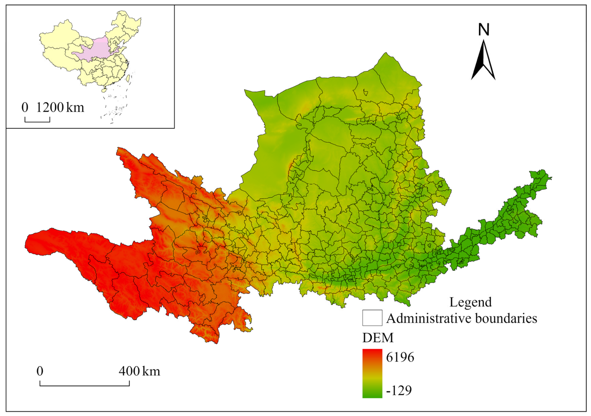
4.1. Spatiotemporal Evolution Patterns of Carbon Emissions

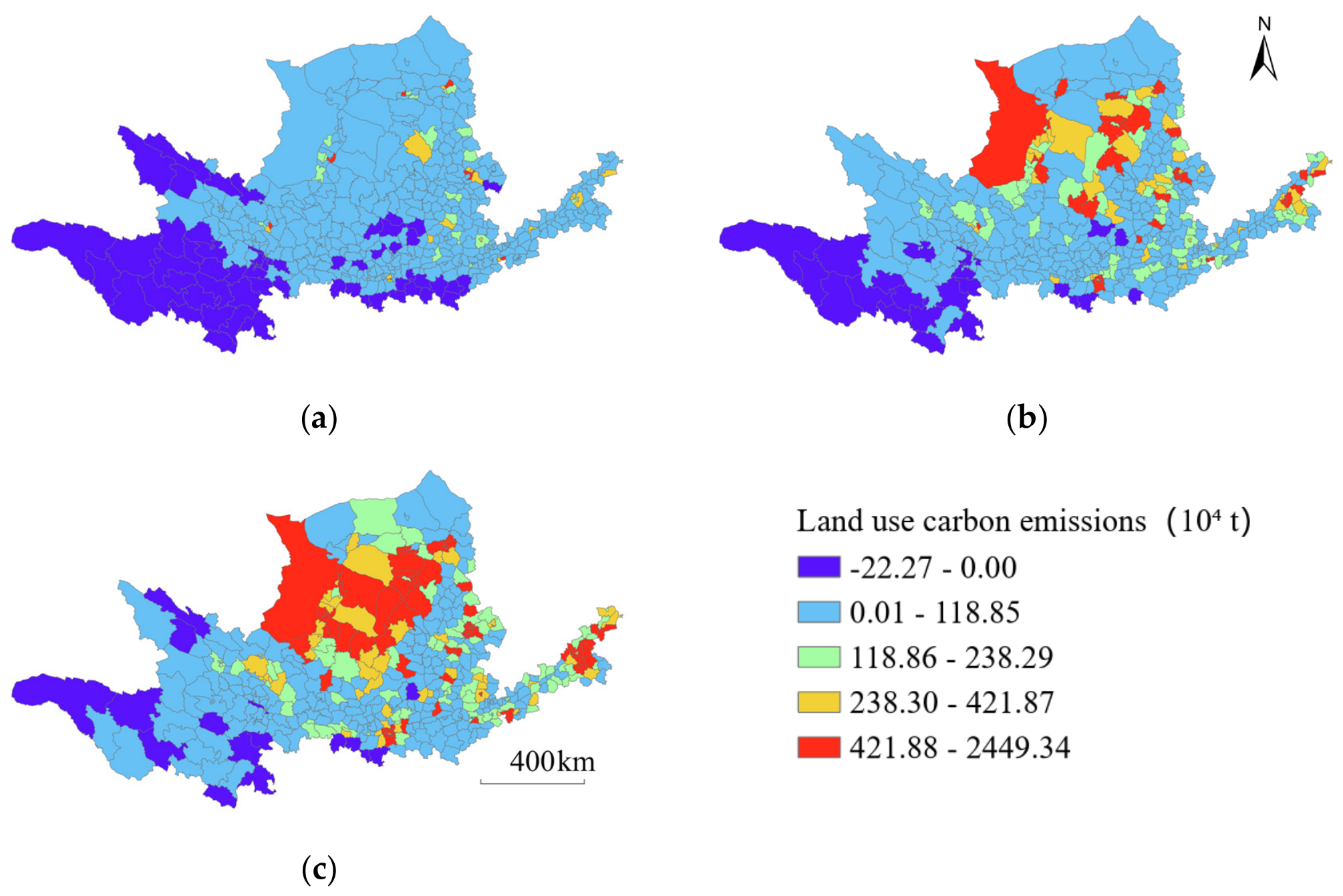
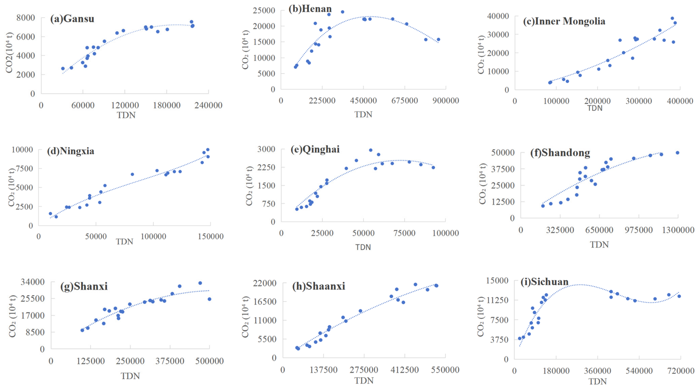
At the county scale, as shown in Figure 4, total land-use carbon emissions in the YRB increased sharply, although the growth rate slowed over time. High-emission areas expanded rapidly, while carbon sink capacity weakened significantly, placing increasing pressure on the overall carbon balance of the basin. Total carbon emissions were 235 million tons, 658 million tons, and 1033 million tons in 2000, 2010, and 2020, respectively. During 2000–2010, rapid urbanization led to a 179% increase in carbon emissions. During 2010–2020, the growth rate slowed to 57%. This slowdown coincided with ecological restoration projects, optimization of the energy structure, improvements in land-use efficiency, and the transition toward high-quality urban development.

Table 6. Proportional distribution of carbon emission intervals at the county scale.

Category	Range (104 t)	2000		2010		2020
		N	%	N	%	N	%
Negative	−22.27–0.00	57	12.61%	23	5.09%	17	3.76%
Low	0.01–118.85	343	75.88%	279	61.73%	235	51.99%
Moderate	118.86–238.29	25	5.53%	68	15.04%	81	17.92%
	238.30–421.87	19	4.20%	39	8.63%	47	10.40%
High	421.88–2449.34	8	1.77%	43	9.51%	72	15.93%
	In total	452	100.00%	452	100.00%	452	100.00%

summarizes the distribution of county-level units across different carbon-emission intervals in 2000, 2010, and 2020. The number of counties with negative net carbon emissions decreased from 57 (12.61%) in 2000 to 23 (5.09%) in 2010 and further to 17 (3.76%) in 2020. Meanwhile, the proportion of counties in the low-emission category declined from 75.88% to 51.99%. In contrast, the combined number of counties in the moderate-emission categories increased from 44 in 2000 to 128 in 2020, while the number of high-emission counties increased from 8 (1.77%) to 72 (15.93%). These changes quantitatively demonstrate a broad shift from negative- and low-emission classes toward moderate- and high-emission classes at the county scale. Spatially, high-emission areas were concentrated at the junction of central Inner Mongolia, northern Ningxia, and northern Shaanxi, showing a clear clustering pattern. This area is rich in energy resources, and carbon emissions from energy consumption constitute the main emission source. County-level units where prefecture-level city seats are located formed secondary high-emission centers. High-emission areas showed rapid expansion.

This indicates that not only did the number of high-emission areas increase, but emissions from individual county-level units also rose sharply. These results are consistent with the spatial concentration of energy-intensive industries in these areas, creating structural challenges for the low-carbon transition. Counties with negative carbon emissions, here referred to as “carbon sink counties”, were mainly concentrated in non-traditional energy areas such as eastern Qinghai and northern Sichuan. The number of carbon sink counties decreased from 57 to 17, a reduction of 40 counties over the 20-year period. This suggests that the net carbon sequestration capacity of natural ecosystems in the YRB has been gradually weakened. With declining carbon sink capacity and increasing carbon emissions, the overall carbon balance pressure in the basin has intensified.

The county-scale analysis reveals the macro-level administrative pattern and overall evolutionary trend of carbon emissions. However, due to the spatial aggregation effect of administrative units, county-level averages may mask internal spatial heterogeneity and fail to capture local spatial details. Therefore, this study further conducted a grid-scale analysis to identify the spatial distribution patterns of carbon emissions from a finer-scale perspective.

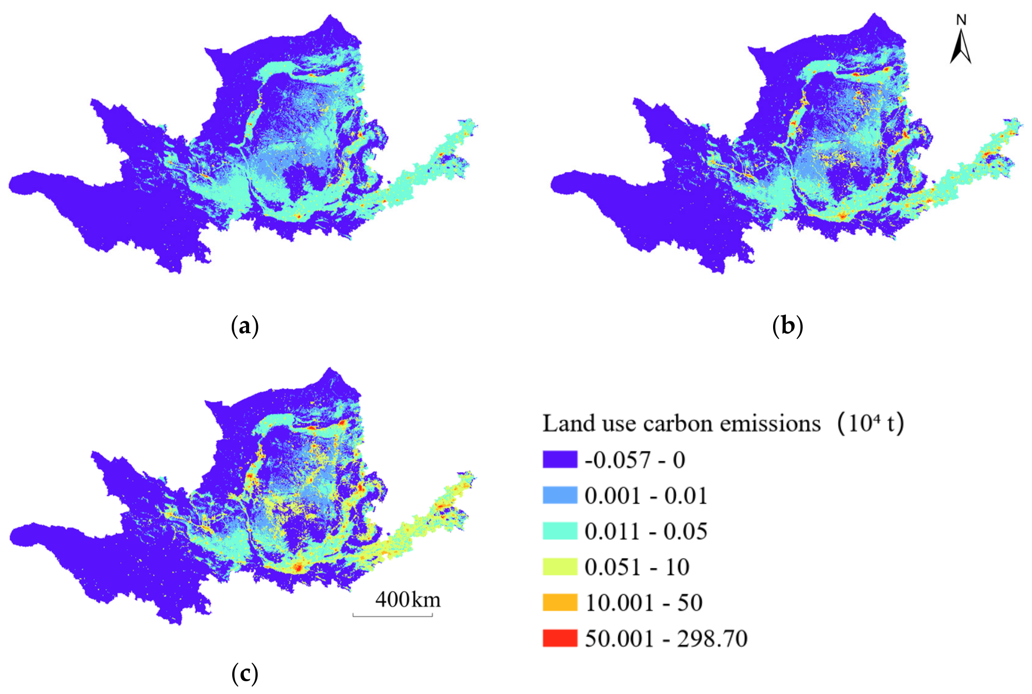
Because the raster data of land-use carbon emissions in the YRB exhibited an obvious skewed distribution, the data were classified into six classes within four major intervals based on their natural attributes. These include the negative-emission interval, or carbon sink interval (−0.057–0); low-emission intervals (0.001–0.01 and 0.011–0.05); the moderate-emission interval (0.051–10); and high-emission intervals (10.001–50 and 50.001–298.702). The classification results are shown in Figure 5, and the proportions of different intervals are presented in

Table 7. Proportional distribution of carbon emission intervals at the grid scale.

Category	Range (104 t)	2000		2010		2020
		N	%	N	%	N	%
Negative	−0.057–0	85,127	61.03%	86,991	62.36%	85,761	61.47%
Low	0.001–0.01	18,648	13.37%	17,095	12.26%	15,161	10.87%
	0.011–0.05	31,229	22.39%	25,443	18.24%	16,871	12.09%
Moderate	0.051–10	4029	2.89%	8305	5.95%	19,495	13.97%
High	10.001–50	368	0.26%	1416	1.02%	1881	1.35%
	50.001–298.702	90	0.06%	241	0.17%	346	0.25%
In total		139,491	100%	139,491	100%	139,491	100%

.

During the study period, the spatial pattern of carbon emissions showed an evolutionary trend characterized by “dominance of carbon sink areas with slight contraction, substantial shrinkage of low-emission areas, and significant expansion of moderate- and high-emission areas.” Among these intervals, moderate-emission areas expanded the fastest, while high-emission areas continued to increase with a considerable absolute increment. This indicates that regional carbon emissions were shifting from low-emission classes toward moderate- and high-emission classes, leading to increasing pressure for emission reduction.

Negative-emission areas were mainly distributed in the western, northern, and northwestern parts of the basin. They remained dominant throughout the study period, with their grid-cell proportion consistently exceeding 60%. The main land-use types in these areas were forestland, grassland, and unused land, indicating that most areas of the YRB functioned as carbon sinks in terms of land-use carbon emissions during the study period. Benefiting from policies such as the Grain for Green Program, the proportion of negative-emission grid cells reached a peak of 62.36% in 2010. However, this proportion declined slightly by 2020, which coincided with accelerated urbanization and cropland conversion.

Low-emission areas were mainly distributed in the middle and lower reaches of the YRB and experienced substantial shrinkage. Their grid-cell proportion decreased from 35.76% in 2000 to 30.50% in 2010 and further to 22.96% in 2020. Among them, the proportion of grid cells with carbon emissions ranging from 0.011 to 0.05 decreased by more than 10 percentage points, while that of grid cells ranging from 0.001 to 0.01 decreased by 2.5 percentage points. This suggests that areas with carbon emissions closer to zero are more likely to maintain their emission status and exhibit stronger stability. This pattern was also associated with relatively stable land-use types.

Moderate-emission areas were mainly distributed in the lower reaches of the basin. Their grid-cell proportion increased sharply from 2.89% to 13.97%, representing an approximately fourfold increase over the 20-year period and making this the fastest-expanding emission interval. Notably, the rapid expansion of moderate-emission areas was highly synchronized in time and space with the substantial shrinkage of low-emission areas. This indicates that many grid cells originally in a low-emission state shifted toward the moderate-emission interval.

High-emission areas were mainly centered around several resource-based cities and expanded significantly over the 20-year period. Although high-emission grid cells accounted for a relatively small proportion, they showed a continuous expansion trend. By 2020, the proportion of high-emission grid cells was 4.86 times that in 2000. Although the growth rate declined from 262% during 2000–2010 to 34% during 2010–2020, the absolute increase remained considerable. Given the large emission values in high-emission areas, especially in areas with emissions greater than 500,000 tons, these areas should receive particular attention in future governance.

4.2. Spatiotemporal Evolution Patterns of ESV

The total ESV of the YRB remained generally stable with a slight upward trend, indicating good macro-level stability. Spatially, ESV showed a gradient distribution, with lower values in the southeast and higher values in the northwest. In terms of ESV changes, however, the number of counties with ESV degradation exceeded that with improvement in the latter decade, showing a pattern of “overall stability but local imbalance.”

From 2000 to 2020, the total ESV of the YRB increased from 2695.15 billion yuan to 2766.70 billion yuan, with an average annual growth rate of approximately 0.13%. Specifically, ESV increased relatively markedly during 2000–2010, with a growth rate of approximately 3.0%. During 2010–2020, it entered a high-level stabilization stage and decreased slightly by approximately 0.35%. Overall, the fluctuation was small, indicating that ecosystem service functions in the basin remained relatively stable at the macro scale.

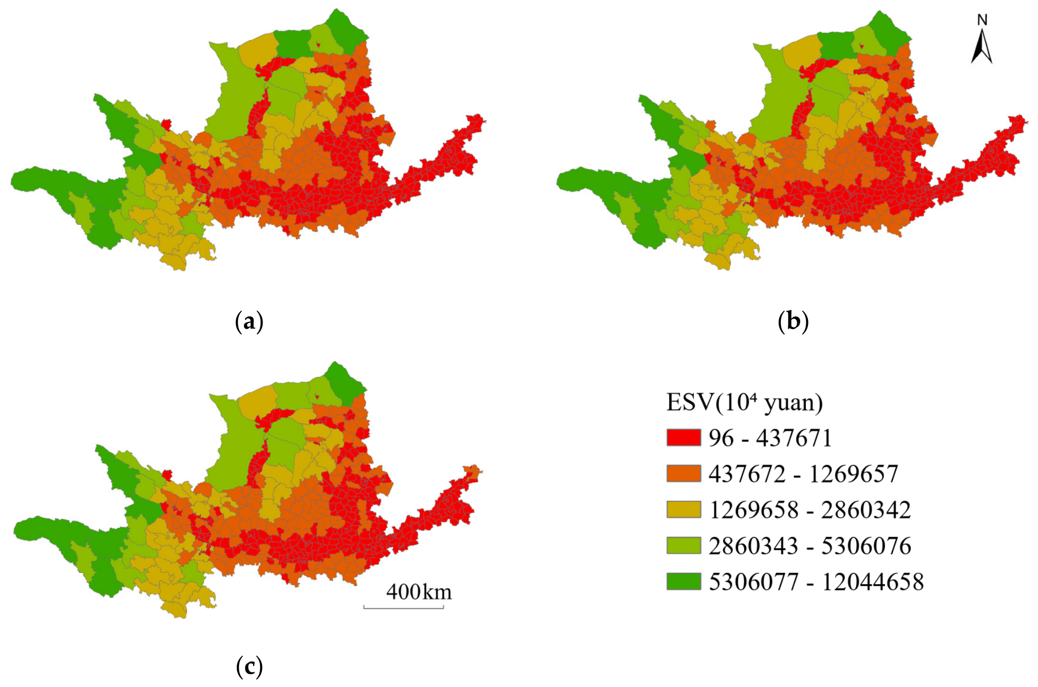
Spatially, ESV gradually increased from the southeast to the northwest, as shown in Figure 6. High-value areas were concentrated in the western and northern parts of the YRB. These areas include ecological function conservation zones such as the source regions of the Yangtze River and the Yellow River and are dominated by natural grassland ecosystems. These areas are characterized by strong ecosystem service functions and relatively high ESV levels. Notably, although Alxa Left Banner in the northwestern part of the basin is dominated by unused land and has a low ESV per unit area, its vast area, combined with the basic services provided by desert ecosystems, such as wind prevention, sand fixation, and biodiversity maintenance, is associated with relatively high total ESV at the basin scale. As a result, it forms a special high-value area at the basin scale.

Low-value areas were widely distributed in the middle and lower reaches of the Yellow River. These areas are densely populated and characterized by frequent agricultural and urban construction activities. Their land-use types are dominated by cropland and artificial construction land, while the proportion of natural ecosystems is relatively low. These areas are characterized by relatively weak ecosystem service functions and low ESV levels. Medium-value areas are located between the high-value and low-value areas, forming a transition zone and reflecting the gradient transition of ecosystem service functions.

Because the total ESV was relatively stable at the county scale, ESV change rates were further calculated to characterize local variations (shown in

Table 8. Distribution of counties across different ESV change rate categories.

Change Rate	2000–2010	2010–2020
<−20%	5	8
−20~−10%	14	32
−10%~0	112	228
0~10%	261	152
10~20%	47	18
>20%	13	14

). During 2000–2010, 131 counties, accounting for 28.98% of all counties, experienced negative ESV growth. During 2010–2020, the number of counties with negative ESV growth increased to 268, accounting for 59.29%. The number of counties with ESV change rates below −10% increased from 19 to 40, whereas the number of counties with change rates above 10% decreased from 60 to 32. These results indicate that although the total ESV of the entire basin changed only slightly, clear trade-offs occurred at the county scale. ESV improvement dominated in the first decade, while in the second decade, the number of degraded counties exceeded that of improved counties. This suggests that the spatial extent of ESV improvement was shrinking, while the risk of ESV degradation was spreading.

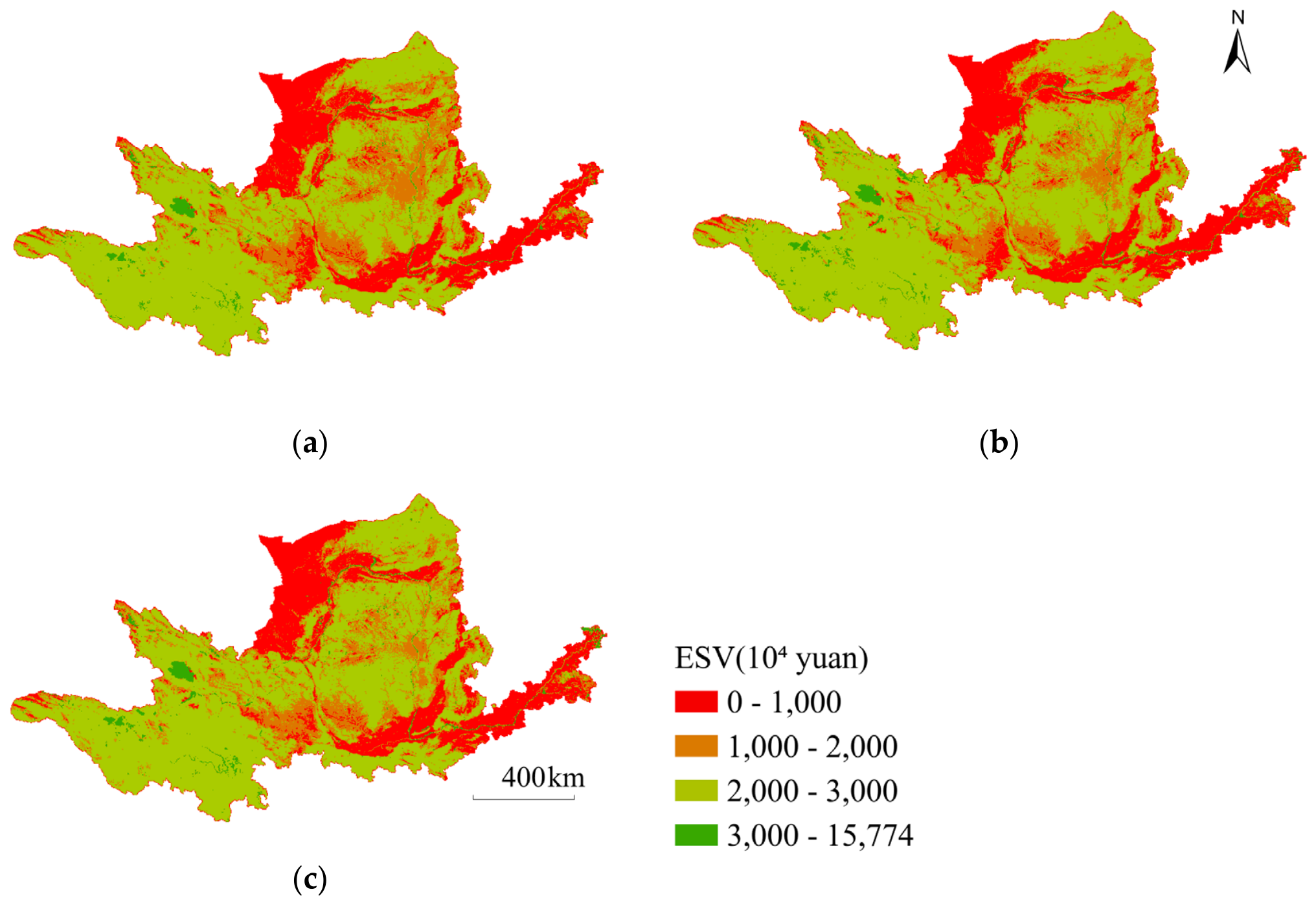
Based on the natural characteristics and variation patterns of the ESV data, the values were classified into four categories: low-value, sub-low-value, moderate-value, and high-value areas, as shown in Figure 7. Overall, the spatial pattern of ESV in the YRB was characterized by “reinforcement of high-value areas and relative stability of middle- and low-value areas.” High-value areas were stably concentrated in the core water conservation areas of the upper reaches, and the number of high-value grid cells continued to increase. Moderate-value areas constituted the dominant ESV category, with their area decreasing first and then remaining stable. Low-value areas were mainly distributed in two large regions, namely the northwestern desert area and the downstream agricultural and urban areas, and their area also showed a trend of first decreasing and then stabilizing.

High-value ESV areas were concentrated in the source region of the upper reaches and remained stably distributed around water bodies and wetlands in eastern Qinghai and northern Sichuan over the long term. These areas constitute the core water conservation zone of the Yellow River and have very strong ecosystem service functions, making them the most stable high-value center in the entire basin. From 2000 to 2010, the number of high-value grid cells increased significantly by 32%. Although the overall number of high-value ESV grid cells experienced a modest decline during 2010–2020, the number of extremely high-value ESV grid cells (ESV > 40 million yuan) remained relatively stable and slightly increased from 1853 in 2010 to 1908 in 2020. This indicates that core ecosystem service areas were maintained despite the reduction in broader high-value regions.

Moderate-value areas were the dominant coverage type in the basin, accounting for more than 55% of the total area. They formed large contiguous zones in the western, northeastern, and southern parts of the basin, as well as in central Shaanxi. These areas were mainly covered by forestland and grassland, and their area decreased during 2000–2010 before becoming stable.

Low-value areas were mainly distributed in two major regions. One was located in the northwestern part of the YRB, corresponding to the desert and sandy areas of Inner Mongolia, where the climate is arid, vegetation cover is low, and ecosystems are highly fragile. The other was located in the Henan and Shandong sections of the Yellow River, as well as central Shaanxi and southern Shanxi. These areas are characterized by dense urban settlements and developed agriculture, with high proportions of cropland and built-up land and a relatively low proportion of natural ecosystems, resulting in significantly lower ESV. The area of low-value zones first decreased and then tended to stabilize. Sub-low-value areas were distributed in patches between the two major low-value regions, and their area also decreased first before becoming stable.

4.3. Spatial Coupling and Correlation of Carbon Emissions and ESV

Analysis of land-use carbon emissions and ESV in the YRB shows that areas with higher carbon emissions tend to have relatively lower ESV, suggesting a possible spatial association between the two variables. To further examine this relationship, GeoDa 1.22 was used to calculate the global bivariate spatial autocorrelation index, and the results are presented in

Table 9. Global bivariate Moran’s I indices between carbon emissions and ESV at the county and grid scales.

Year	County Scale			Grid Scale
	I	p	z	I	p	z
2000	−0.148	<0.001	−6.8094	−0.049	<0.001	−49.0729
2010	−0.118	<0.001	−5.36	−0.082	<0.001	−85.3447
2020	−0.088	<0.001	−4.098	−0.092	<0.001	−95.296

. Across all study years and at both spatial scales, Moran’s I values were negative, with all p-values below 0.001. This indicates a significant negative spatial correlation between land-use carbon emissions and ESV in the YRB at the 99% confidence level. In other words, areas with high carbon emissions tend to be spatially associated with neighboring areas with low ESV, and vice versa.

At the county scale, Moran’s I increased from −0.148 to −0.088, indicating that the negative spatial clustering between carbon emissions and ESV gradually weakened. At the grid scale, however, Moran’s I decreased from −0.049 to −0.092, indicating that the negative spatial correlation gradually strengthened. Compared with the county scale, the grid scale reduces the influence of administrative boundary aggregation and better captures local spatial heterogeneity. The increasing absolute value of Moran’s I suggests that the spatial separation between high-carbon-emission areas and high-ESV areas became increasingly pronounced over the 20-year study period. Specifically, areas with higher carbon emissions were increasingly associated with lower ESV in surrounding areas, whereas areas with higher ESV tended to be surrounded by areas with lower carbon emissions.

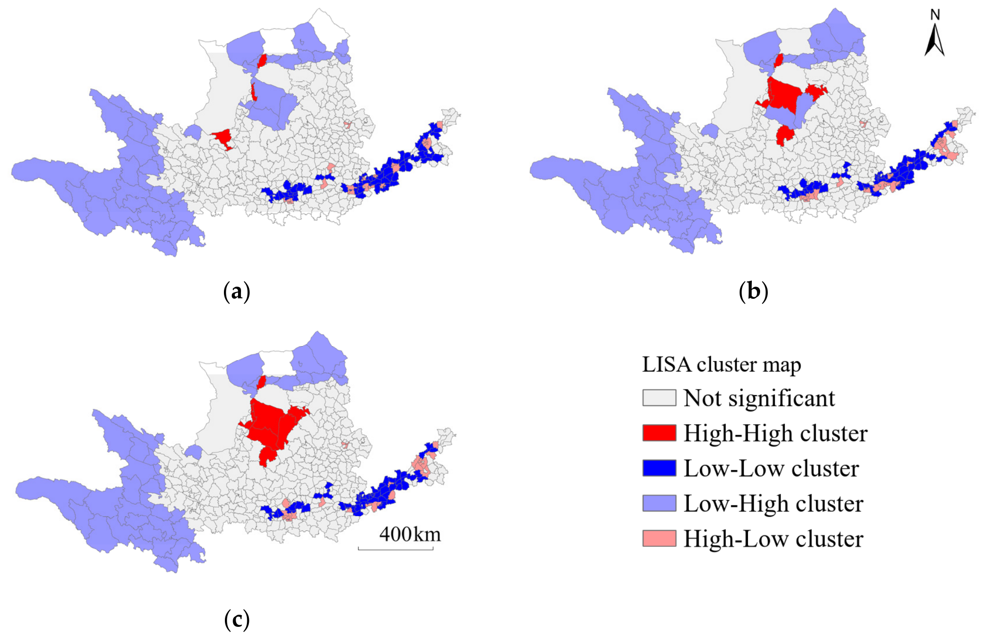
Further analysis using local bivariate Moran’s I, as shown in Figure 8, indicates that the carbon–ESV spatial association in the YRB was dominated by L–H clusters, which were continuously distributed in the ecological coordination areas of the western and northern basin. H–H clusters showed an increasingly grouped distribution in the Ordos–Yulin region, L–L clusters remained stable in a belt across the middle and lower reaches, and H–L clusters appeared as point-like patches embedded in urban built-up areas.

Table 10. Statistics of bivariate LISA cluster types at the county scale in 2000, 2010, and 2020.

LISA Cluster Type	2000		2010		2020
	N	%	N	%	N	%
High–High cluster	4	0.88%	7	1.55%	9	1.99%
Low–Low cluster	62	13.72%	59	13.05%	63	13.94%
Low–High cluster	44	9.73%	42	9.29%	41	9.07%
High–Low cluster	36	7.96%	38	8.41%	31	6.86%
Not significant	306	67.70%	306	67.70%	308	68.14%
In total	452	100%	452	100%	452	100%

summarizes the county-level bivariate LISA results. The number of statistically significant counties remained relatively stable, changing from 146 in both 2000 and 2010 to 144 in 2020. Among the four cluster types, L–L clusters were the most prevalent, accounting for approximately 13–14% of all counties throughout the study period. L–H clusters decreased slightly from 44 (9.73%) to 41 (9.07%), while H–L clusters decreased from 36 (7.96%) to 31 (6.86%). H–H clusters remained limited in number but increased from 4 (0.88%) to 9 (1.99%). Overall, the county-scale cluster structure was comparatively stable, with only modest changes in the numbers of the major cluster types.

Specifically, L–H clusters were distributed as large and continuous patches in some county-level units in the western and northern YRB. This distribution coincides with extensive grassland, forestland, wetlands, and water-conservation ecosystems, as well as relatively limited built-up land and energy-intensive activities, resulting in low local carbon emissions and comparatively high surrounding ESV. The number of county-level units in this category decreased slightly from 44 to 41, mainly because some county-level units in southern Ordos gradually evolved from L–H clusters into H–H clusters. This shift coincided with increasing carbon emissions together with relatively higher surrounding ESV in Ordos, a typical energy city, during the process of rapid industrialization and urbanization.

H–H clusters increased from 4 counties in 2000 to 9 in 2020 and gradually formed a more concentrated distribution in southern Ordos and western Yulin. Under the adopted variable order, this pattern indicates counties with high carbon emissions surrounded by areas with relatively high ESV. This pattern is closely related to the coexistence of intensive energy development and ecological restoration in the region.

L–L clusters were distributed in a continuous belt across parts of central-western Shandong, northeastern Henan, southern Shanxi, and central Shaanxi. This belt-like clustering pattern remained stable over the long term, with only slight changes along the margins. The distribution reflects low-emission cropland areas embedded within surrounding low-ESV landscapes influenced by intensive human activities.

H–L clusters were distributed as point-like patches embedded within the L–L cluster belt, and most of them were county-level units where the seats of prefecture-level cities are located. These counties generally contain a high concentration of built-up land, dense settlements, and intensive economic activity, while neighboring landscapes contain relatively low proportions of high-ESV land-cover types.

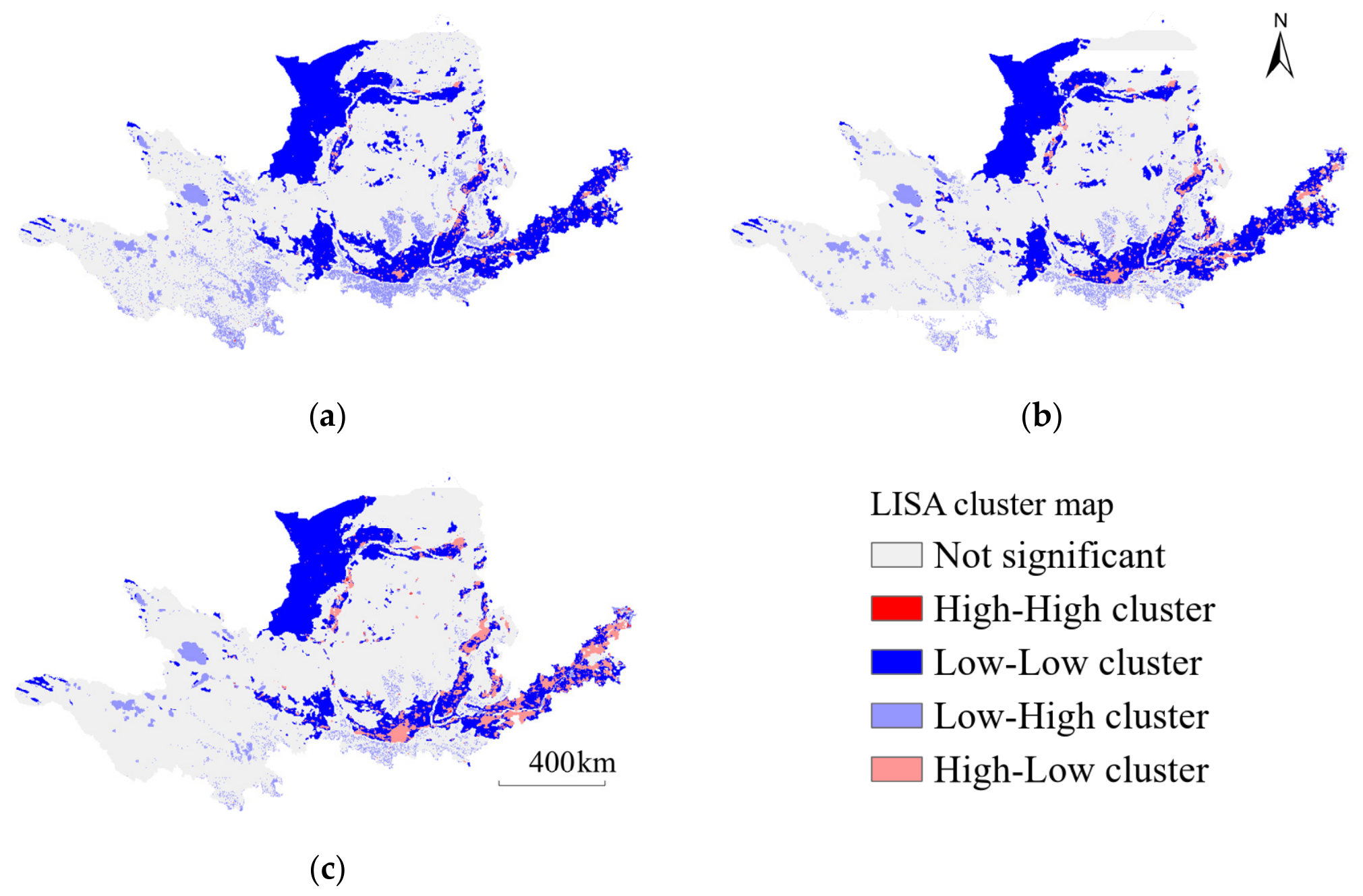
At the grid scale, as shown in Figure 9, the carbon–ESV spatial association in the YRB was dominated by L–L clusters, but their extent decreased substantially over time. L–H clusters declined markedly in the western basin, highlighting the risks of patch fragmentation and the breakdown of carbon sink–ecological synergy. Meanwhile, H–L clusters expanded from the eastern to the central basin, gradually encroaching upon L–L clusters. These grid-scale dynamics reveal the fine-scale carbon emission pressures associated with urbanization and industrialization, as well as the fact that localized declines in carbon–ESV synergy are masked by the averaging effect at the county scale. The grid-scale statistics in

Table 11. Statistics of bivariate LISA cluster types at the grid scale in 2000, 2010, and 2020.

LISA Cluster Type	2000		2010		2020
	N	%	N	%	N	%
High–High cluster	61	0.04%	66	0.05%	127	0.09%
Low–Low cluster	32,103	23.23%	28,998	20.98%	25,699	18.60%
Low–High cluster	12,374	8.96%	7619	5.51%	5436	3.93%
High–Low cluster	2213	1.60%	3768	2.73%	6976	5.05%
Not significant	91,434	66.17%	97,734	70.73%	99,947	72.33%
In total	138,185	100%	138,185	100%	138,185	100%

Note: During the bivariate LISA analysis, grid cells located at the edge of the study area that lacked first-order Queen neighboring relationships were excluded because spatial autocorrelation analysis requires valid spatial connections among units. Therefore, the number of grid cells used in the LISA analysis was slightly smaller than the total number of grid cells reported in Table 7. This treatment only removed boundary cells without valid neighboring information and ensured the validity of spatial autocorrelation calculations.

reveal much greater temporal changes than those observed at the county scale. The number of L–H grid cells decreased from 12,374 (8.96%) in 2000 to 5436 (3.93%) in 2020, representing a decline of 5.03%. Over the same period, H–L grid cells increased from 2213 (1.60%) to 6976 (5.05%), an increase of 3.45%. L–L grid cells declined from 32,103 (23.23%) to 25,699 (18.60%), whereas H–H grid cells increased from 61 to 127, although their overall proportion remained below 0.1%. The proportion of statistically non-significant grid cells also increased from 66.17% to 72.33%. These results demonstrate substantial fine-scale restructuring of the carbon–ESV spatial association pattern.

Specifically, L–L clusters were mainly distributed in large and contiguous patches in the northwestern YRB and along the northern edge of the Yellow River’s J-shaped bend, and also in belt-like zones in the eastern and southern basin. In the north, these L–L clusters were mainly composed of unused land such as desert areas, with extremely low carbon emissions and spatial associations with neighboring areas characterized by low ESV. In the east, L–L clusters were mainly cropland, with relatively low carbon emissions, but they were surrounded by low-ESV grids associated with urban construction and other land uses. Although both belong to the L–L category, the northwestern desert areas mainly result from natural environmental constraints with intrinsically low carbon emissions and low ESV, whereas the eastern agricultural areas reflect low-emission cropland embedded within surrounding low-ESV landscapes influenced by intensive human activities. These two L–L patterns therefore represent different ecological processes.

L–H clusters were mainly distributed in the western and southern YRB, showing an overall pattern of “mottled patches in the west and scattered distribution in the south.” In the western basin, these areas were mainly composed of forestland, grassland, and water conservation areas and lacked large-scale urban and industrial development. Their carbon emissions were extremely low, while neighboring areas exhibited relatively high ESVs, providing the basis for surrounding high ESV. Their mottled distribution pattern was associated with discontinuous ecological spaces and localized human disturbances, which further intensified patch fragmentation. In the south, L–H clusters were mainly distributed in forestland areas, characterized by extremely low carbon emissions and spatial associations with neighboring areas of high ESV.

The extent of L–H clusters decreased by more than 56%. In particular, many L–H clusters in the western basin were transformed into statistically non-significant areas. This suggests hidden risks of ecological fragmentation, localized ESV decline, and breakdown of the carbon sink–ecological synergy pattern in the upstream ecological region. However, the averaging effect of county-level administrative units smooths out internal ecological differences, thereby masking these fragmented but important signals of declining carbon–ESV spatial synergy and failing to reflect the weakening trend of the upstream ecological barrier.

H–L clusters were distributed in belt-like zones in the eastern YRB and as expanding patches in the central basin, showing a gradual tendency to encroach upon L–L clusters. In 2000, H–L clusters were only sporadically distributed in belts in the east. By 2010, they had extended toward the central basin, and by 2020 they formed a pattern of “eastern belts + central patches,” deeply embedded within the L–L cluster pattern. This indicates that the carbon emission pressures brought about by urbanization and industrialization become particularly evident at fine spatial scales, and these details cannot be fully captured at the county scale.

A direct comparison of the two spatial scales further demonstrates the scale-dependent nature of the carbon–ESV association. Between 2000 and 2020, the number of county-level L–H clusters decreased by only 0.66% (from 44 to 41), whereas the number of grid-level L–H clusters decreased by 5.03% (from 12,374 to 5436). Similarly, county-level H–L clusters decreased by 1.10% (from 36 to 31), while grid-level H–L clusters increased by 3.45% (from 2213 to 6976). County-level L–L clusters remained nearly unchanged, increasing from 62 to 63 (+0.22%), whereas grid-level L–L clusters declined from 32,103 to 25,699 (−4.63%). In addition, the proportion of statistically non-significant units increased by only 0.44 percentage points at the county scale but by 6.16 percentage points at the grid scale. These contrasting changes indicate that county-level aggregation produces a comparatively stable macro-pattern, while the grid analysis captures substantial localized restructuring in synergistic and conflicting carbon–ESV associations.

4.4. Zoning for the Synergistic Governance of Carbon Emissions and ESV

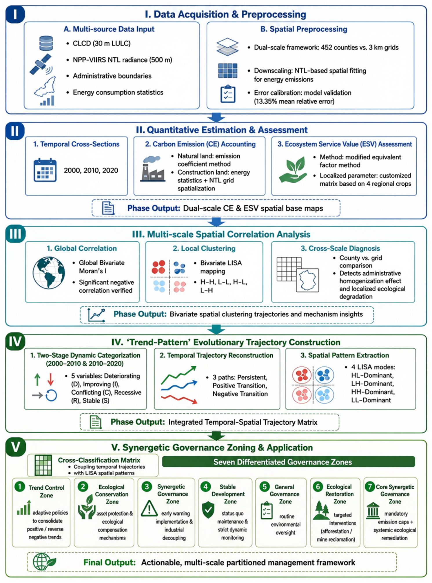
To achieve synergistic governance of carbon-emission reduction and ecological protection in the YRB, this study developed a two-dimensional Trend–Pattern zoning framework at the grid scale. The framework integrates the dynamic changes in carbon emissions and ESV during two periods, 2000–2010 and 2010–2020, with the spatial association characteristics identified by bivariate LISA. Based on this framework, the study area was ultimately divided into seven types of differentiated governance zones, providing a basis for targeted policy implementation in the basin.

4.4.1. Zoning Method and Workflow

The Trend–Pattern framework integrates temporal trend trajectories derived from carbon emission–ESV dynamics with spatial patterns represented by dominant bivariate LISA clusters, thereby providing the conceptual basis for governance zoning. Because the framework relies on the direction of temporal evolution and spatial association patterns rather than predefined numerical thresholds, the zoning results are not affected by arbitrary threshold selection. Therefore, conventional threshold sensitivity analysis is not directly applicable. The zoning procedure included four steps: classifying change types, constructing change trajectories, coupling them with spatial association trajectories, and conducting cross-classification. The specific steps are described as follows.

(1)

Classification of carbon-emission and ESV change types

The dynamic changes in carbon emissions and ESV were calculated for two periods: 2000–2010 and 2010–2020. Positive values (>0) were classified as increases, negative values (<0) as decreases, and zero values (=0) as unchanged. Because both carbon emissions and ESV were calculated as continuous variables without discretization, the classification was based on the direction of temporal change rather than arbitrary magnitude thresholds. Accordingly, grid cells were classified into five change types according to their change characteristics, as defined in

Table 12. Classification standards for the dynamic changes of carbon emissions and ESV.

Change Type	Abbreviation	Description
Deteriorating	D	Increased carbon emissions & decreased ESV; or constant carbon emissions & decreased ESV
Improving	I	Decreased carbon emissions & increased ESV; or decreased carbon emissions & Constant ESV; or constant carbon emissions & increased ESV
Conflicting	C	Increased carbon emissions & increased ESV; or increased carbon emissions & constant ESV
Recessive	R	Decreased carbon emissions & decreased ESV
Stable	S	Constant carbon emissions & constant ESV

. In this classification, the Trend dimension emphasizes the directional evolution of carbon emissions–ESV relationships rather than the magnitude of numerical changes. Therefore, slight variations between consecutive periods are interpreted as part of the overall temporal trajectory, while the final governance zoning is further determined by integrating the Trend dimension with spatial Pattern characteristics derived from bivariate LISA analysis.

(2)

Construction of two-stage change trajectories

For each grid cell, the change types in the two periods, 2000–2010 and 2010–2020, were integrated. According to the objectives of coordinated ecological protection and carbon-emission reduction, the five change types were ranked from most to least favorable as follows: improvement type > stability type > conflict type > decline type > deterioration type. The improvement type represents the most desirable trajectory, characterized by decreasing carbon emissions with increasing or stable ESV, or increasing ESV with stable carbon emissions. The stability type indicates that both carbon emissions and ESV remain unchanged. The conflict type reflects continued carbon-emission growth despite maintained or improved ESV. The decline type represents simultaneous decreases in both carbon emissions and ESV, indicating a reduction in ecosystem service provision despite reduced emissions. The deterioration type is the least desirable condition, as ESV decreases while carbon emissions increase or remain unchanged. Based on this ranking, the combinations of change types across the two periods were further classified into three trajectory categories.

The first category is the persistent trajectory, in which the change type remained the same in both periods. This category includes persistent deterioration (DD), persistent improvement (II), persistent conflict (CC), persistent decline (RR), and persistent stability (SS). The second category is the improving transition trajectory, in which the change type in the second period was more favorable than that in the first period, such as a transition from conflict type to stability type, indicating that the coordinated relationship tended to improve. The third category is the deteriorating transition trajectory, in which the change type in the second period was less favorable than that in the first period, such as a transition from stability type to conflict type, indicating a potential risk of weakened coordination.

(3)

Construction of bivariate LISA spatial association trajectories

Based on the bivariate local spatial autocorrelation results for carbon emissions and ESV in 2010 and 2020, as described in Section 4.3, two-stage LISA trajectories were constructed and classified into five types.

The HL-dominant type refers to grid cells that were classified as H–L clusters in at least one of the two years and were never classified as L–H clusters. The LH-dominant type refers to grid cells that were classified as L–H clusters in at least one of the two years and were never classified as H–L clusters. The H–H dominant type refers to grid cells that were never classified as H–L, L–H, or L–L clusters, and were classified as H–H clusters in at least one year. The LL-dominant type refers to grid cells that were never classified as H–L, L–H, or H–H clusters, and were classified as L–L clusters in at least one year. All remaining combinations were classified as other types.

(4)

Coupled cross-classification and delineation of governance zones

The two-stage change trajectories were coupled with the LISA spatial association trajectories to construct a cross-classification matrix, as shown in

Table 13. Cross-classification matrix and spatial synergistic zoning.

Combined Change Type	HL	LH	HH	LL	Others
Persistent Deterioration	Core SGZ	ERZ	Core SGZ	SGZ	SGZ
Positive Transformation	TCZ	ECZ	TCZ	TCZ	TCZ
Negative Transformation	SGZ	TCZ	SGZ	TCZ	TCZ
Persistent Improvement	GGZ	ECZ	GGZ	GGZ	ECZ
Persistent Conflict	SGZ	GGZ	SGZ	GGZ	GGZ
Persistent Recession	GGZ	ERZ	GGZ	ERZ	GGZ
Persistent Stability	SDZ	SDZ	SDZ	SDZ	SDZ

Note: Core SGZ: Core Synergistic Governance Zone; ERZ: Ecological Restoration Zone; SGZ: Synergistic Governance Zone; TCZ: Trend Control Zone; ECZ: Ecological Conservation Zone; GGZ: General Governance Zone; SDZ: Stable Development Zone.

. Based on the coordinated characteristics and governance needs of different categories, seven synergistic governance zones were delineated. These seven zones represent the minimum set of categories required to distinguish the major combinations of temporal evolution trajectories and dominant spatial association patterns while maintaining practical interpretability for governance. Fewer categories would merge areas with distinct governance priorities, whereas additional categories would increase complexity without providing substantial management value. Each governance zone was identified from two complementary dimensions: (1) the temporal evolution trajectory represented by the combined change types, reflecting long-term carbon–ecological dynamics; and (2) the dominant LISA spatial association category, including HL, LH, HH, LL, and Others, indicating the current spatial interaction between carbon emissions and ESV. By integrating temporal dynamics with present spatial characteristics, the cross-classification matrix provides a basis for identifying differentiated governance priorities. For example, areas with persistent deterioration and an HL-dominant pattern indicate both a worsening temporal trajectory and a spatial association between high carbon emissions and neighboring low-ESV areas; therefore, they were classified as the Core Synergistic Governance Zone. Although Trend Control Zone, General Governance Zone, and Synergistic Governance Zone all require management intervention, they differ conceptually. Trend Control Zone emphasizes trajectory regulation because these areas are undergoing positive or negative transitions before stable spatial patterns are established. General Governance Zone represents relatively moderate combinations that do not exhibit pronounced ecological advantages or severe carbon–ecology conflicts and therefore require routine management. In contrast, the Synergistic Governance Zone identifies areas where unfavorable temporal trajectories coincide with conflict-prone spatial associations, making coordinated carbon-emission reduction and ecological management the primary governance objective.

4.4.2. Zoning Results and Spatial Distribution Characteristics

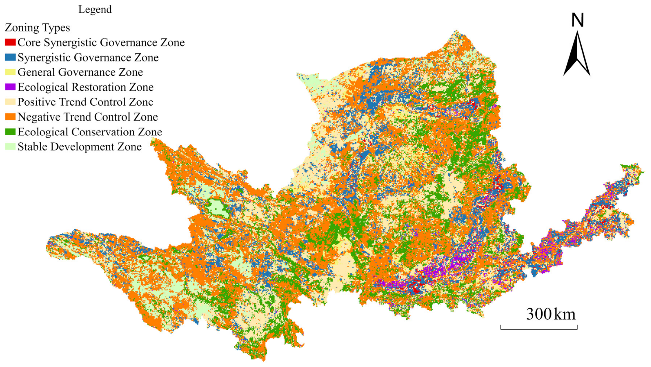
Based on the above method, the spatial zoning map of synergistic governance in the YRB was generated, as shown in Figure 10. The area proportions, main characteristics, and management strategies of each zone are presented in

Table 14. Grid statistics and management strategies for each spatial governance zone.

Zone		Grid Count	Proportion (%)	Characteristics and Management Strategies
Trend Control Zone	Positive	56,559	40.93%	The synergistic relationship is undergoing a positive transition, but the advantages of spatial clustering have not yet fully emerged. Consolidate the transition gains and prevent trend reversal.
	Negative	28,515	20.64%	The synergistic relationship is undergoing a negative transition, but no significant high-risk spatial clustering has yet emerged. Strengthen early-warning interventions and promptly contain and reverse the adverse trend.
Ecological Conservation Zone		20,595	14.9	Continuous improvement or positive transformation in ecological advantage areas. Strengthen ecological compensation and strictly control ecological land conversion in upstream ecological barriers.
Synergistic Governance Zone		14,206	10.28	Includes units with non-typical spatial correlation but deteriorating trends, or those in stress/H–H areas. Prioritize industrial upgrading in energy bases and urban expansion control in metropolitan areas.
Stable Development Zone		7566	5.48	Long-term stable units. Maintain current status and strengthen routine monitoring.
General Governance Zone		6553	4.74	Other combination types. Implement routine management and standard environmental oversight.
Ecological Restoration Zone		2271	1.64	Areas with continuous recession/deterioration in ecological advantage or L–L regions. Prioritize abandoned mine restoration, vegetation reconstruction, and watershed ecological restoration.
Core Synergistic Governance Zone		1920	1.39	Continuously deteriorating units in H–L or H–H spatial clusters. Strictly control high-energy-consuming industries and implement integrated emission reduction and ecological restoration.

.

Overall, the trend control zones remained the dominant governance type, accounting for more than 60% of the total area, with positive trend control zones (40.93%) substantially exceeding negative trend control zones (20.64%). Ecological conservation zones and synergistic governance zones were the next most extensive categories, together accounting for 25.18%. Although core synergistic governance zones and ecological restoration zones accounted for less than 4% of the total area, they represent key and challenging areas for basin governance.

In terms of spatial distribution, the synergistic governance zoning of the basin was characterized by widely distributed and contiguous dominant types, point-like clustering of special types, and a clear differentiation between ecological zones and conflict-prone zones.

Specifically, positive trend control zones were widely distributed across the basin and represented areas undergoing a positive transition in the carbon–ecology relationship despite the absence of dominant spatial clustering. Governance in these areas should focus on consolidating the ongoing transition, preventing reversal, and gradually strengthening carbon–ecology synergies. Negative trend control zones, in contrast, represented areas experiencing an unfavorable transition before the emergence of significant high-risk spatial clustering. These areas require strengthened monitoring, early-warning interventions, and timely management measures to prevent further deterioration into conflict-prone governance zones. Representative counties include Qin’an County, Jia County, and Zhuanglang County for the positive TCZ, and Zuoyun County, Jingchuan County, and Yijun County for the negative TCZ.

Ecological conservation zones were mainly concentrated in ecologically advantageous areas in the middle and upper reaches. Representative counties include Pianguan County, Hequ County, and Jingle County. These areas were mostly LH-dominant units characterized by persistent improvement or improving transition, and they constitute the core functional areas for ESV supply in the basin. Governance in these areas should focus on ecological protection, establishment of ecological compensation mechanisms, promotion of green development experience, and enhancement of ecosystem carbon sink functions.

Synergistic governance zones were mainly distributed in densely urbanized areas and energy development areas in the middle and lower reaches. Representative counties include Hanggin Rear Banner, Zhongmu County, and Linhe District. These areas were H–H aggregation units characterized by persistent conflict or deteriorating transition, where the contradiction between carbon emissions and ecological protection was particularly prominent. Governance in these areas should seek low-carbon development pathways by optimizing the industrial structure and controlling urban expansion, so as to alleviate the conflict between increasing carbon emissions and ecological protection.

Stable development zones were mainly distributed in parts of the western and northern YRB. Representative counties include Gangcha County, Zeku County, and Dari County. These areas have remained in a long-term stable state of carbon–ecology coordination and are subject to relatively weak human disturbance. Governance should strictly control new development activities, strengthen ecological and carbon monitoring, and prevent external disturbances from undermining the existing stable pattern.

The General Governance Zone is scattered and interspersed throughout the basin, often occurring among other zones such as the Trend Regulation Zone and the Coordinated Governance Zone, without forming any obvious large-scale contiguous clusters. Representative counties include Xiji County, Uxin Banner, and Binzhou City. It mainly comprises residual combinations with no distinct evolutionary trends or spatial association characteristics, and the overall carbon–ecological conflict is relatively weak. Routine management should therefore be implemented, together with strengthened dynamic monitoring and appropriate control of development intensity, to prevent a shift toward conflict or degradation.

Ecological restoration zones were scattered in central Shaanxi and southern Shanxi, with a tendency to develop into contiguous belt-like areas. Representative counties include Linyi County, Dali County, and Fufeng County. These areas were LH-dominant or LL-dominant zones characterized by persistent decline or deterioration, and they face a significant risk of ESV loss. Governance should implement projects such as forest and grassland restoration, wetland protection, and mine-site revegetation to improve ecosystem stability.

Core synergistic governance zones were scattered in the lower reaches of the YRB and in resource-based cities in the middle and upper reaches. Representative counties include Yanta District, Yuquan District, and Weicheng District. These areas were persistently deteriorating HL/HH-dominant units and exhibited the most pronounced carbon–ecological management challenges due to unfavorable temporal trajectories combined with conflict-prone or high-pressure spatial association patterns. Governance in these areas should adopt mandatory control measures, strictly limit the scale of energy-intensive industries, and promote the coordinated implementation of low-carbon transition and ecological restoration.

Overall, the zoning pattern is generally consistent with the major functional regions of the YRB. Ecological Conservation Zones are mainly distributed within the upper-reach ecological barrier and important ecological conservation areas, whereas Synergistic Governance Zones and Core Synergistic Governance Zones largely coincide with major energy-development areas and densely urbanized regions in the middle and lower reaches. This spatial consistency indicates that the proposed Trend–Pattern framework effectively captures the dominant regional carbon–ecology characteristics while providing finer-scale management information within existing planning frameworks.

Although the proposed zoning framework is developed at the grid scale to capture fine spatial heterogeneity, practical implementation should be coordinated with existing county-level administrative systems. Therefore, the grid-based results are intended to support intra-county identification of priority management areas rather than replace current administrative planning units. Future applications may further integrate grid-scale diagnosis with administrative governance mechanisms to improve operational feasibility.

While Table 14 summarizes the recommended governance strategies for each zone, the proposed framework is intended to provide a diagnostic and decision-support basis for differentiated management rather than prescribe uniform quantitative regulatory targets. Specific carbon-emission reduction ratios or ESV enhancement thresholds should be determined by local governments according to regional emission baselines, ecosystem conditions, industrial structures, and ongoing carbon-neutrality policies. Consequently, the governance recommendations proposed in this study should be regarded as adaptive management priorities that can be further developed into locally appropriate implementation targets.

5. Discussion

5.1. Key Findings

This study systematically analyzed the spatiotemporal evolution and spatial association between land-use carbon emissions and ESV in the YRB from 2000 to 2020 at both the county and 3 km × 3 km grid scales, based on land-use data. Furthermore, by coupling the dynamic changes in carbon emissions and ESV with the spatial association characteristics identified by bivariate LISA, this study developed a two-dimensional Trend–Pattern synergistic governance zoning framework at the grid scale. The main findings not only reveal the dynamic evolution of the carbon–ecological system in the YRB at the empirical level, but also provide several mechanistic and policy implications that merit further discussion.

The results show that total carbon emissions in the YRB surged from 235 million tons to 1.033 billion tons during 2000–2020, accompanied by a rapid increase in the number of high-emission counties. In contrast, total ESV increased only slightly from 2695.147 billion yuan to 2766.704 billion yuan, with an average annual growth rate of only 0.13%. This indicates an asymmetric pattern characterized by a sharp increase in carbon emissions and marginal growth in ESV. More importantly, although ESV remained generally stable with a slight upward trend at the county scale, and high-value ESV areas even continued to be reinforced at the grid scale, the grid-scale bivariate LISA analysis revealed that L–H ecological coordination clusters decreased by more than 56% and showed a trend of patch fragmentation in the western basin. These findings suggest that the carbon–ecological conflict in the YRB is not manifested as synchronized deterioration across the entire basin. Rather, it is characterized by local mismatches under overall stability and the hidden weakening of ecological coordination areas. Conventional assessments based on administrative units may substantially underestimate the risk of functional weakening in the upstream ecological barrier due to the averaging effect. Therefore, fine-scale spatial association analysis provides important complementary information for detecting potential localized declines in carbon–ESV synergy that may be less apparent at the administrative scale.

These scale-dependent differences can be explained by several underlying spatial mechanisms. First, county-level assessments are affected by the MAUP, whereby spatial aggregation smooths local variability and masks ecological hotspots through averaging within administrative boundaries [49]. Second, the YRB exhibits pronounced landscape heterogeneity, with forests, croplands, urban land, and water bodies frequently coexisting within individual counties. Aggregating these heterogeneous land-use types into a single administrative unit inevitably reduces the ability to detect localized carbon–ecological conflicts [50]. Third, ecological processes and land-use interactions operate continuously across space rather than following administrative boundaries [49]. Consequently, grid-based analysis can provide a finer representation of the spatial coupling between anthropogenic activities and ecosystem functions and can reveal localized degradation signals that may be less apparent at the county scale. These mechanisms explain why the grid-scale analysis identified the substantial contraction of L–H clusters, whereas the county-scale assessment suggested only limited changes.

5.2. Comparison with Existing Research

The finding that total carbon emissions continued to increase while the growth rate slowed, together with the continuous expansion of medium- and high-emission areas, is consistent with previous studies on carbon emissions in the YRB [43,46,47]. Meanwhile, the relative stability of total ESV, supported by ecological restoration projects such as the Grain for Green Program, also agrees with the results of most existing assessments [51,52,53]. In terms of the spatial association between carbon emissions and ESV, many studies have reported a negative spatial correlation between the two variables [25,28,54]. By comparing the county scale with the 3 km grid scale, this study provides important extensions to these findings.

First, this study reveals scale heterogeneity and the averaging effect. At the grid scale, carbon emissions showed a hierarchical transition characterized by carbon sink contraction, low-emission area shrinkage, and medium- and high-emission area expansion. However, the slowdown in emission growth observed at the county scale may have weakened the visibility of these fine-scale pressures. Similarly, although total ESV remained relatively stable, the grid-scale analysis showed that the carbon–ecological synergy in the upstream region had weakened markedly. This risk was less evident in county-level administrative units because of the averaging effect.

Second, this study challenges the assumption that macro-level ESV stability necessarily indicates ecological security. Stability in the total amount of ESV does not mean that functional coordination is secure. Greater attention should therefore be paid to the dynamic early warning of coordinated relationships at fine spatial scales. Overall, this study highlights the potential information loss associated with relying solely on administrative-scale assessments and provides complementary multi-scale information for carbon–ecological governance in the YRB.

The proposed Trend–Pattern framework also differs from widely adopted territorial spatial planning approaches, such as the “Three Zones and Three Lines” and the Ecological Red Line. These planning frameworks primarily delineate functional spaces based on ecological protection priorities, agricultural production, and urban development, providing a relatively static basis for territorial spatial management [55,56]. In contrast, the Trend–Pattern framework emphasizes the dynamic interactions between carbon emissions and ESV by integrating both temporal evolution and spatial association. This enables the identification of areas undergoing improvement, deterioration, or persistent carbon–ecological conflicts, thereby supporting adaptive governance rather than static spatial control. Furthermore, the incorporation of grid-scale analysis allows localized ecological risks that are obscured by administrative-scale assessments to be detected. Therefore, rather than replacing existing zoning systems, the proposed framework provides a complementary decision-support tool that can help refine differentiated governance strategies within established territorial planning frameworks. Specifically, ecological red lines identify areas requiring strict protection, whereas the Trend–Pattern framework further prioritizes management actions according to the evolutionary trajectory of carbon–ecological interactions, thereby providing additional support for adaptive ecological governance under changing environmental conditions.

5.3. Research Contributions and Policy Implications

This study first integrates county- and grid-scale assessments with the evolution of bivariate spatial associations, revealing the phenomenon of “localized mismatch under overall stability” and highlighting the potential limitations of single-scale analyses in studies of the coupling relationship between ecosystem services and carbon emissions. The proposed masking mechanism of the averaging effect further enriches the theoretical understanding of the relationship between scale selection and landscape pattern processes.

Based on the spatial association types and evolutionary trajectories of carbon emissions and ESV, seven governance zones were delineated to support differentiated spatial planning and management. Ecological conservation zones should prioritize ecological protection and maintain landscape connectivity through ecological compensation and strict conservation measures. Stable development zones should maintain current land-use patterns while strengthening long-term monitoring to detect potential disturbances. Trend control zones require adaptive management, with planning measures tailored to local trajectories by consolidating improvements in recovering areas and introducing timely interventions in deteriorating areas. Synergistic governance zones should optimize industrial layout, regulate development intensity, and establish early-warning systems to prevent the expansion of carbon–ecological conflicts. General governance zones should maintain existing management practices while continuing routine environmental monitoring. Ecological restoration zones should prioritize forest and grassland restoration, mine-site revegetation, and other nature-based solutions to enhance ecosystem services. Core synergistic governance zones should be designated as priority areas for coordinated emission reduction and ecological restoration, with strict land-use control, restoration targets, and implementation monitoring integrated into regional planning frameworks.

The proposed governance zones are generally consistent with China’s current territorial spatial planning framework and ecological governance strategies. For example, Ecological Conservation Zones correspond to areas prioritizing ecological protection and ecosystem conservation, whereas Ecological Restoration Zones are consistent with national ecological restoration initiatives. Trend Control Zones are aligned with carbon-emission reduction policies targeting rapidly urbanizing regions. Therefore, the proposed zoning framework provides a practical decision-support tool that complements existing land-use policies rather than replacing them.

Although developed for the YRB, the Trend–Pattern framework is not region-specific. It can be transferred to other river basins where multi-temporal carbon-emission and ecosystem-service datasets are available and where spatial heterogeneity plays an important role in carbon–ecological interactions. Nevertheless, the specific zoning results and management priorities should be adjusted according to local ecological conditions, land-use characteristics, and governance objectives.

5.4. Research Limitations and Future Directions

Although this study systematically reveals the spatial association between carbon emissions and ESV in the YRB, several limitations remain and require further exploration in future research.

First, the carbon emission accounting boundary is not yet fully comprehensive. This study focused on land-use carbon emissions. Carbon emissions from built-up land were spatially estimated using energy consumption statistics and NTL data, thereby implicitly representing energy-related emissions associated with industrial production, residential activities, and transportation. However, industrial process emissions (e.g., cement clinker calcination and chemical production) and emissions associated with agricultural and livestock production that fall outside the adopted land-use carbon accounting framework were not explicitly included [57,58]. It should be noted that energy-related emissions from industrial activities have been partially captured through provincial energy consumption statistics and NTL-based spatialization, whereas non-energy industrial process emissions remain outside the current accounting boundary. This limitation may lead to a certain underestimation of carbon emissions in some areas of the YRB. Future studies could integrate sector-specific emission inventories with land-use carbon accounting to construct a more comprehensive grid-based carbon emission accounting framework. Moreover, although independent municipal carbon-emission inventories would provide additional validation for the spatialized emission estimates, such datasets are currently unavailable for the entire YRB. Future studies could incorporate publicly available municipal carbon inventories to further evaluate the robustness of the proposed spatialization framework.

In addition, uncertainty may also arise from the NTL-based spatial downscaling procedure. Although the regression models were calibrated using provincial energy consumption statistics, NTL intensity cannot fully represent the spatial distribution of all energy-consuming activities, particularly in industrial areas with weak lighting signals or rural production areas. Consequently, the locations and boundaries of individual grid-scale carbon-emission hotspots may contain spatial allocation uncertainty, which may further influence local LISA classifications and the resulting governance-zone boundaries. Furthermore, the 3 km grid was selected to balance spatial heterogeneity, data consistency, and computational efficiency, but different spatial resolutions may produce different local spatial association patterns due to scale effects. Finally, the Trend–Pattern zoning framework is based on temporal trajectories and dominant LISA patterns; therefore, the zoning results may vary with alternative spatial resolutions or future changes in land-use patterns. Accordingly, the identified grid-scale hotspots and governance zones should be interpreted as relative spatial patterns and management-priority areas rather than precise local emission inventories or rigid regulatory boundaries.

Second, there are limitations in the ESV assessment. This study adopted the equivalent factor method because of its relatively simple data requirements and its suitability for macro-scale ESV assessments based on land-use change. Although the standard equivalent values were regionalized according to the agricultural production characteristics of the YRB, uniform equivalent coefficients were assigned to each land-use type across the study area. Consequently, the method cannot fully capture environmental heterogeneity within the same land-use type, as ESV may vary with local topographic, climatic, and soil conditions. In addition, because the equivalent factor method estimates ESV using standardized equivalent coefficients derived from agricultural production values, the resulting ESV should be regarded as a monetary proxy rather than a direct measurement of ecosystem functioning or ecological processes. Accordingly, it provides an integrated indicator of the relative capacity of ecosystems to deliver services under a unified valuation framework, but cannot fully capture the non-market, multidimensional, and process-based characteristics of ecosystem functioning. Furthermore, the estimated ESV is sensitive to the selected equivalent coefficients, particularly for cropland, grassland, wetlands, and water bodies. Since no sensitivity analysis of the equivalent coefficients was conducted in this study, the influence of coefficient uncertainty on the estimated ESV was not explicitly evaluated and should therefore be acknowledged as a limitation. However, because this study primarily focuses on the spatial coupling patterns between carbon emissions and ESV rather than the absolute valuation of ecosystem services, these uncertainties are unlikely to substantially affect the identified spatial association patterns or the resulting governance zoning. Future studies could improve ESV assessment by incorporating spatially and temporally differentiated correction factors based on elevation, precipitation, soil properties, and other environmental variables, integrating process-based models such as InVEST with multiple valuation approaches, and conducting sensitivity analyses of key equivalent coefficients to further evaluate the robustness of the results.

Third, the bivariate LISA analysis identifies spatial association patterns rather than causal relationships between carbon emissions and ESV. The observed spatial correlations may also be influenced by other factors, such as socioeconomic development, industrial structure, ecological restoration policies, and natural environmental conditions. Therefore, the identified spatial patterns should be interpreted as diagnostic evidence of spatial coupling rather than direct evidence of causal mechanisms. Future studies could integrate spatial regression or structural equation models to further investigate the drivers of carbon–ESV interactions.

The methodology adopted in this study is primarily based on established carbon-accounting methods, standardized ecosystem service valuation coefficients, and mature spatial statistical approaches. Most methodological parameters were adopted directly from widely accepted studies rather than calibrated during model development. Therefore, the uncertainty associated with subjective parameter selection is relatively limited. Future studies may further evaluate the influence of alternative emission coefficients, ecosystem service valuation parameters, or spatial resolutions through formal sensitivity analyses as more region-specific datasets become available.

Finally, the temporal coverage of this study is limited to 2000–2020. The three temporal cross-sections were intentionally selected to examine the decadal spatiotemporal evolution of carbon emissions and ESV over two comparable ten-year periods. It may therefore not reflect the latest impacts of China’s accelerated energy structure transition following the implementation of the “dual carbon” goals, the large-scale development of wind and solar energy, or integrated restoration projects for mountains, rivers, forests, farmland, lakes, grasslands, and deserts in the YRB. Future research will extend the dataset to 2025 and further develop scenario-based projections toward 2030 to evaluate more recent changes in the carbon–ESV relationship, thereby providing a more timely scientific basis for adaptive management in the YRB.

6. Conclusions

This study developed a multi-scale analytical framework integrating land-use data, NTL imagery, and statistical energy consumption data to investigate the coupled dynamics between land-use carbon emissions and ESV in the YRB. By combining temporal evolution trends with spatial association patterns, a Trend–Pattern framework was proposed to support differentiated synergistic governance and bridge the gap between spatiotemporal diagnosis and practical land-use management.

The results revealed pronounced asymmetry in the evolution of carbon emissions and ecosystem services during 2000–2020. Total carbon emissions increased dramatically from 235 million tons to 1.033 billion tons, whereas total ESV remained relatively stable with only slight fluctuations. Although carbon emissions and ESV exhibited a significant negative spatial correlation, substantial scale effects were identified. County-scale analysis captured the overall spatial evolution of carbon emissions and ecosystem services, whereas grid-scale analysis revealed considerable local heterogeneity and changes in carbon–ESV spatial relationships that were masked by administrative averaging. In particular, the marked contraction of L–H clusters demonstrates that relying solely on administrative units may underestimate localized carbon–ecological conflicts and overlook emerging ecological risks.

Beyond these empirical findings, this study provides several methodological contributions. First, the proposed multi-scale analytical framework systematically compares county-scale administrative units with grid-scale natural spatial units, revealing how spatial scale influences the interpretation of carbon–ecological relationships. Second, the Trend–Pattern framework extends conventional bivariate spatial association analysis by integrating temporal trajectories with spatial patterns. Rather than merely identifying spatial clusters, it translates coupled carbon–ESV dynamics into governance-oriented diagnoses and provides a decision-support basis for differentiated management. Third, by coupling temporal trajectories with dominant spatial association patterns, this study delineates seven governance zones with explicit management objectives and corresponding policy recommendations, thereby advancing previous studies from descriptive spatial pattern analysis toward decision-support-oriented governance zoning.

The findings also provide important implications for decision making and regional sustainable development. First, differentiated governance strategies should complement uniform administrative management because different regions exhibit distinct carbon–ecological trajectories and spatial association characteristics. Areas characterized by persistent carbon–ecological conflicts require stricter emission reduction measures, industrial restructuring, and energy transition, whereas ecological conservation zones should prioritize maintaining ecosystem integrity and preventing future degradation. Second, the identified scale effects suggest that grid-scale remote sensing monitoring should complement conventional county-level assessments to improve the early detection of possible localized ecological degradation and carbon–ecological conflicts. Finally, the proposed Trend–Pattern framework provides a transferable decision-support tool for ecological compensation, land-use optimization, and low-carbon transition planning in large river basins and other regions facing the dual challenges of ecological conservation and socioeconomic development.