Author Contributions
Conceptualization, D.P. and Q.Z.; Methodology, D.P., G.S., J.W., L.H., Q.Z. and H.Z.; Software, D.P.; Validation, D.P., G.S., J.W., L.H., Q.Z. and H.Z.; Formal analysis, D.P. and L.H.; Investigation, D.P., G.S. and J.W.; Resources, D.P. and J.W.; Data curation, D.P. and L.H.; Writing—original draft, D.P.; Writing—review & editing, D.P., G.S., L.H., Q.Z. and H.Z.; Visualization, D.P.; Supervision, G.S., J.W. and H.Z.; Project administration, D.P. and H.Z.; Funding acquisition, H.Z. All authors have read and agreed to the published version of the manuscript.
Figure 1.
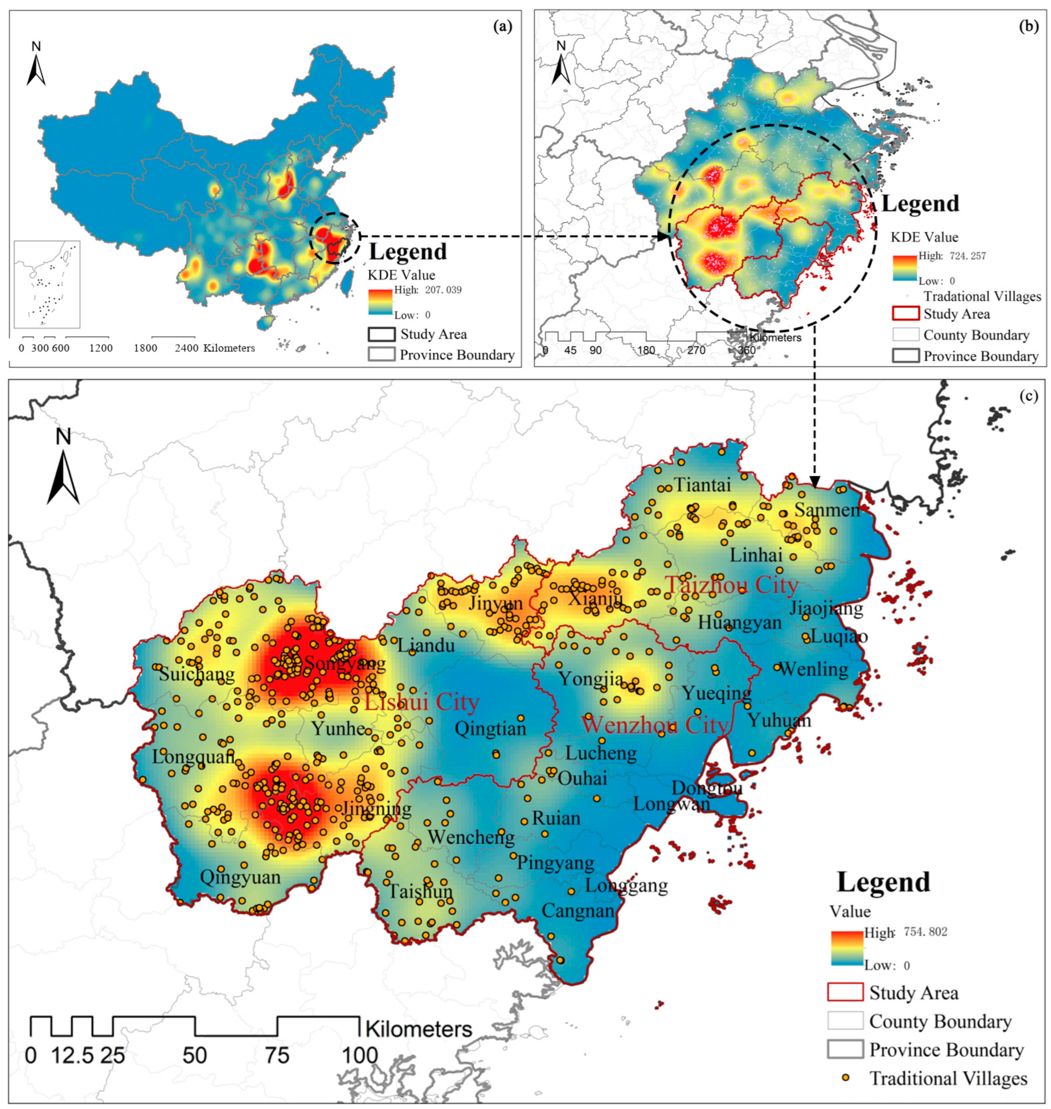
Descriptive conventional ArcGIS KDE patterns of recognized traditional villages in (a) China, (b) Zhejiang Province, and (c) southern Zhejiang. The three independently scaled cartographic surfaces provide regional context only; their values are not compared across panels, and none is used as the model outcome.
Figure 1.
Descriptive conventional ArcGIS KDE patterns of recognized traditional villages in (a) China, (b) Zhejiang Province, and (c) southern Zhejiang. The three independently scaled cartographic surfaces provide regional context only; their values are not compared across panels, and none is used as the model outcome.
Figure 2.
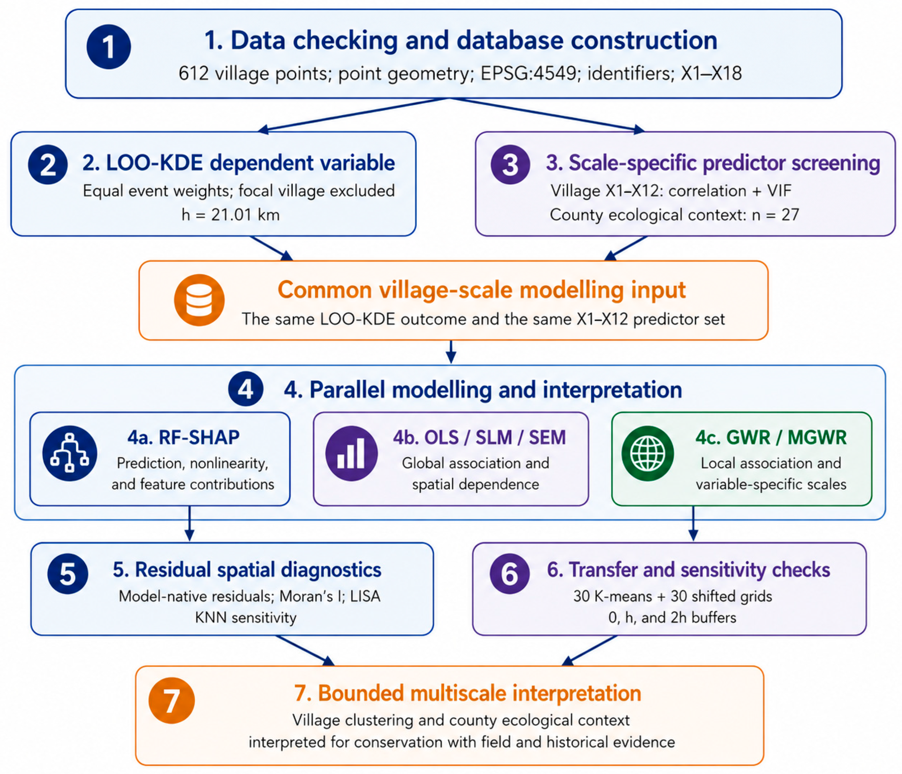
Implemented scale-aware analytical workflow. The workflow separates construction of the self-excluding LOO-KDE outcome, village-scale X1–X12 modelling, 27-unit county ecological context, model-native residual diagnostics, and repeated spatial transfer and sensitivity checks. The final interpretation is explicitly bound to the correlates of local clustering intensity.
Figure 2.
Implemented scale-aware analytical workflow. The workflow separates construction of the self-excluding LOO-KDE outcome, village-scale X1–X12 modelling, 27-unit county ecological context, model-native residual diagnostics, and repeated spatial transfer and sensitivity checks. The final interpretation is explicitly bound to the correlates of local clustering intensity.
Figure 3.
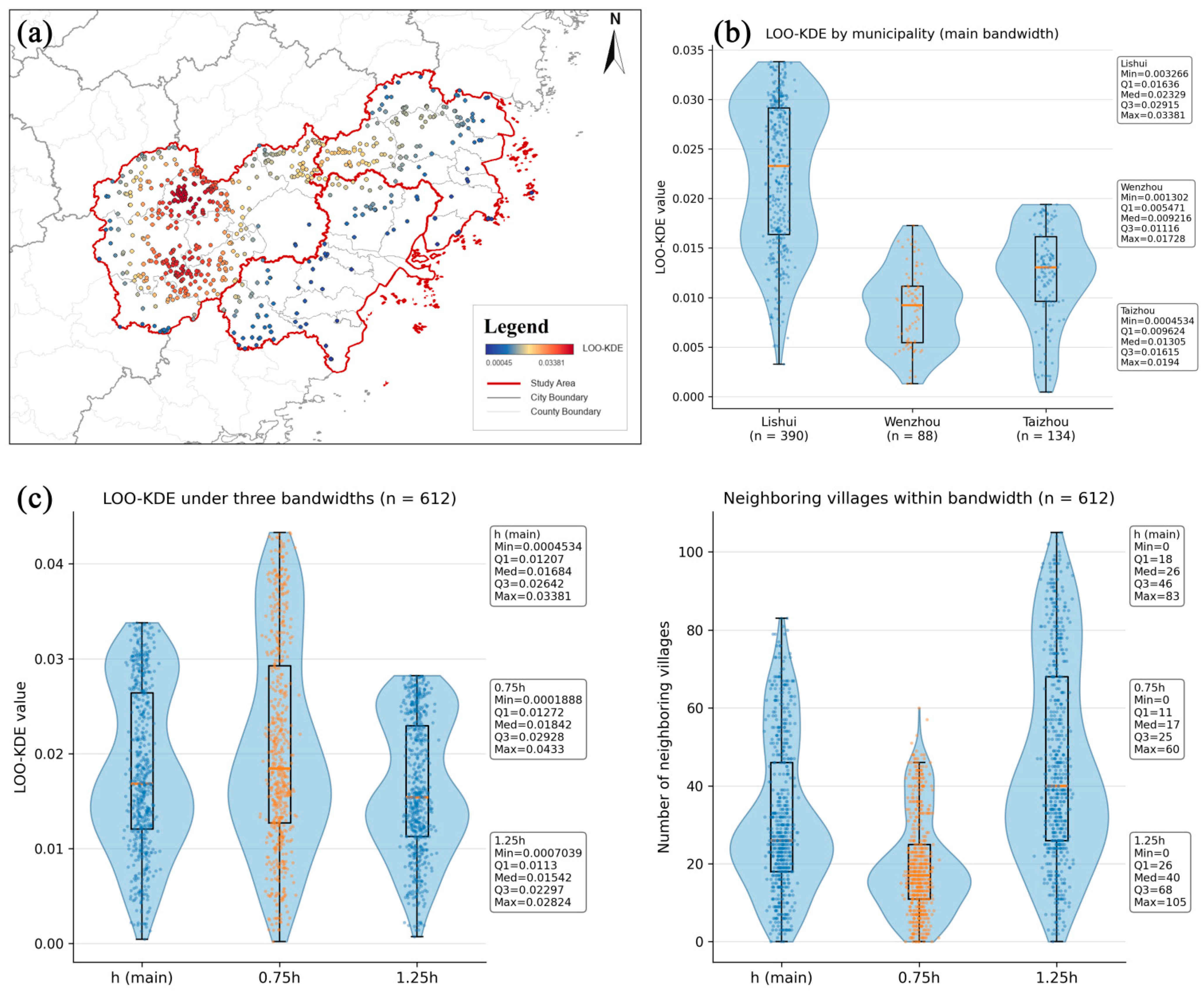
Local clustering intensity of the 612 recognized traditional villages in southern Zhejiang: (a) spatial distribution of LOO-KDE; (b) violin and box plots of LOO-KDE by municipality; (c) violin and box plots of LOO-KDE and of the number of neighbouring villages within the bandwidth, under the main, 0.75 h, and 1.25 h bandwidths.
Figure 3.
Local clustering intensity of the 612 recognized traditional villages in southern Zhejiang: (a) spatial distribution of LOO-KDE; (b) violin and box plots of LOO-KDE by municipality; (c) violin and box plots of LOO-KDE and of the number of neighbouring villages within the bandwidth, under the main, 0.75 h, and 1.25 h bandwidths.
Figure 4.
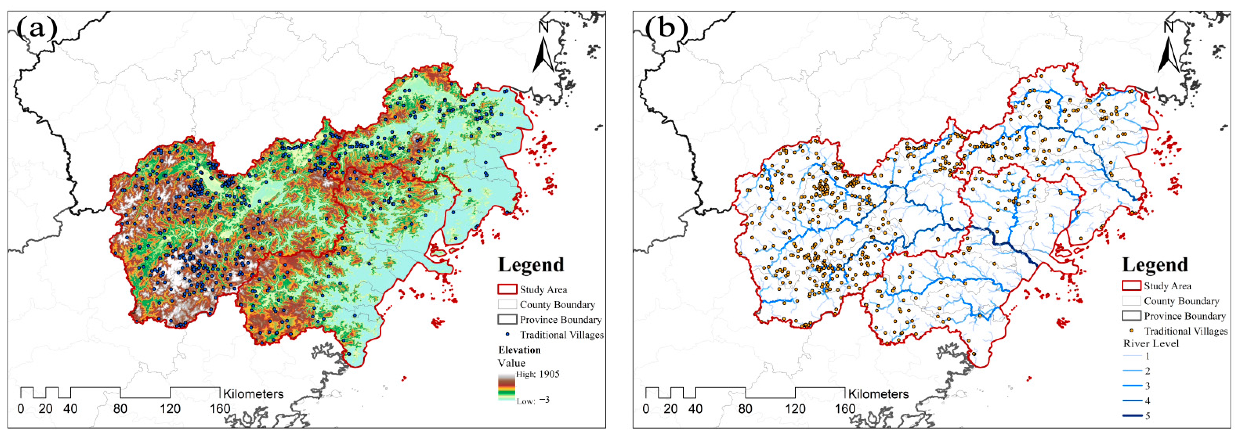
Relationship between traditional village distribution and topographic–hydrological conditions in southern Zhejiang: (a) relationship between traditional village distribution and elevation in southern Zhejiang; (b) relationship between traditional village distribution and river networks in southern Zhejiang.
Figure 4.
Relationship between traditional village distribution and topographic–hydrological conditions in southern Zhejiang: (a) relationship between traditional village distribution and elevation in southern Zhejiang; (b) relationship between traditional village distribution and river networks in southern Zhejiang.
Figure 5.
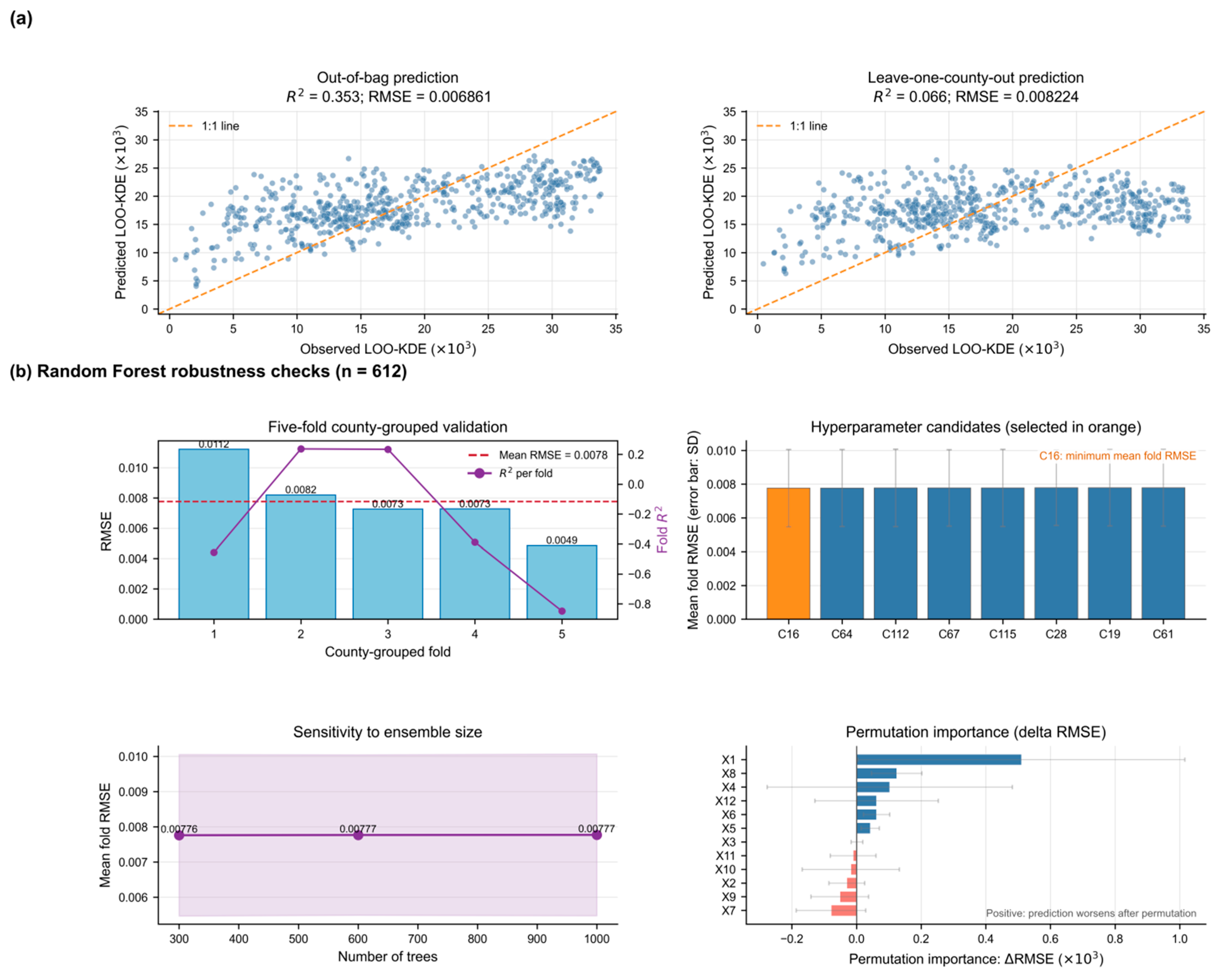
Random Forest diagnostics for the final X1–X12 model. (a) Observed-versus-predicted LOO-KDE for out-of-bag prediction and leave-one-county-out transfer; dashed orange lines show 1:1 agreement. (b) Robustness checks comprising five-fold county-grouped validation, the leading candidates from the 144-combination tuning search (selected candidate in orange), ensemble-size sensitivity, and county-grouped test-set permutation importance expressed as the change in RMSE. Error bars denote between-fold standard deviations.
Figure 5.
Random Forest diagnostics for the final X1–X12 model. (a) Observed-versus-predicted LOO-KDE for out-of-bag prediction and leave-one-county-out transfer; dashed orange lines show 1:1 agreement. (b) Robustness checks comprising five-fold county-grouped validation, the leading candidates from the 144-combination tuning search (selected candidate in orange), ensemble-size sensitivity, and county-grouped test-set permutation importance expressed as the change in RMSE. Error bars denote between-fold standard deviations.
Figure 6.
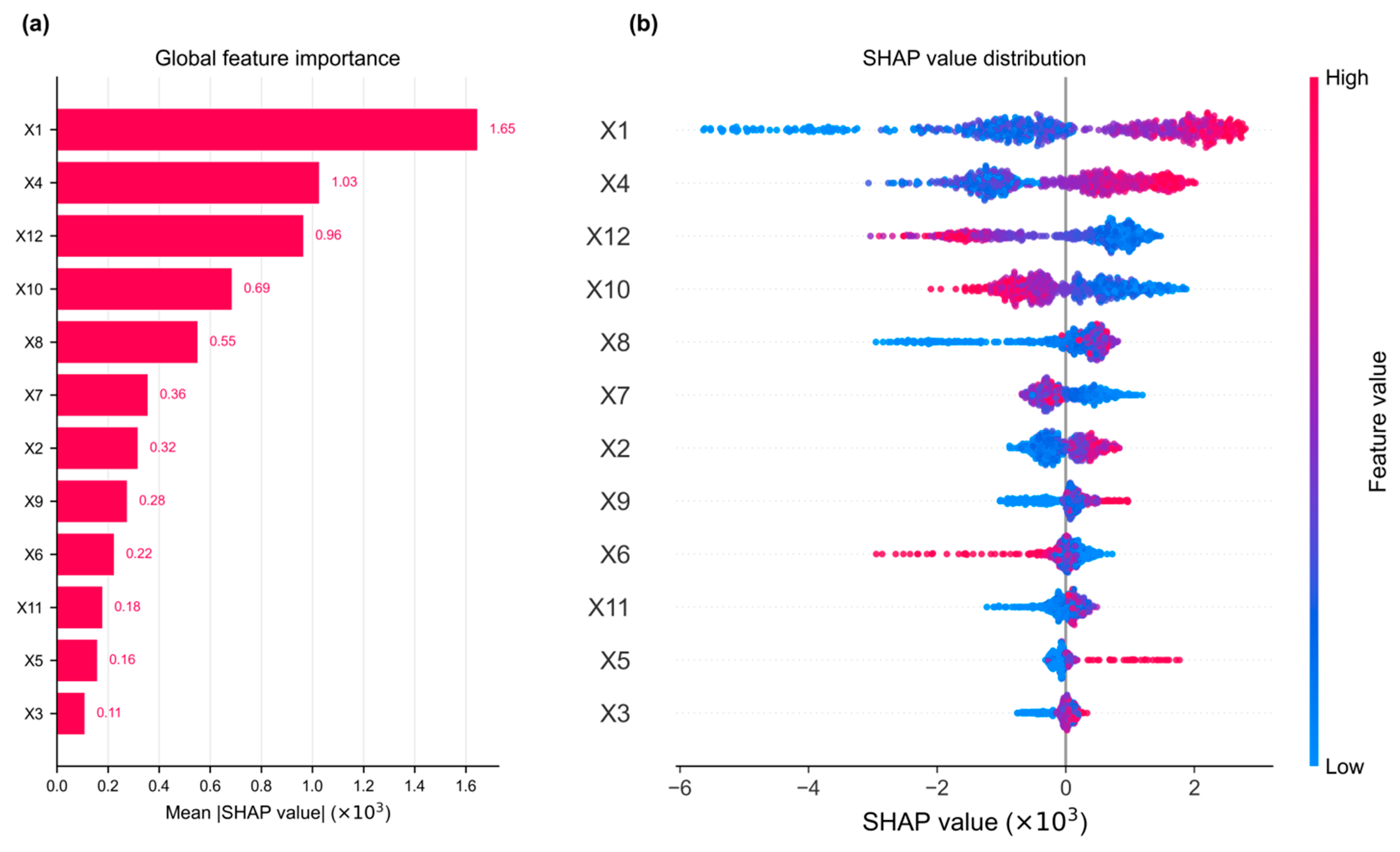
TreeSHAP interpretation of the final X1–X12 Random Forest: (a) mean absolute SHAP importance and (b) beeswarm distribution. The common blue–purple–magenta scale denotes observed feature values from low to high. SHAP values are multiplied by 103 for legibility only; rankings, signs, and model results are unchanged.
Figure 6.
TreeSHAP interpretation of the final X1–X12 Random Forest: (a) mean absolute SHAP importance and (b) beeswarm distribution. The common blue–purple–magenta scale denotes observed feature values from low to high. SHAP values are multiplied by 103 for legibility only; rankings, signs, and model results are unchanged.
Figure 7.
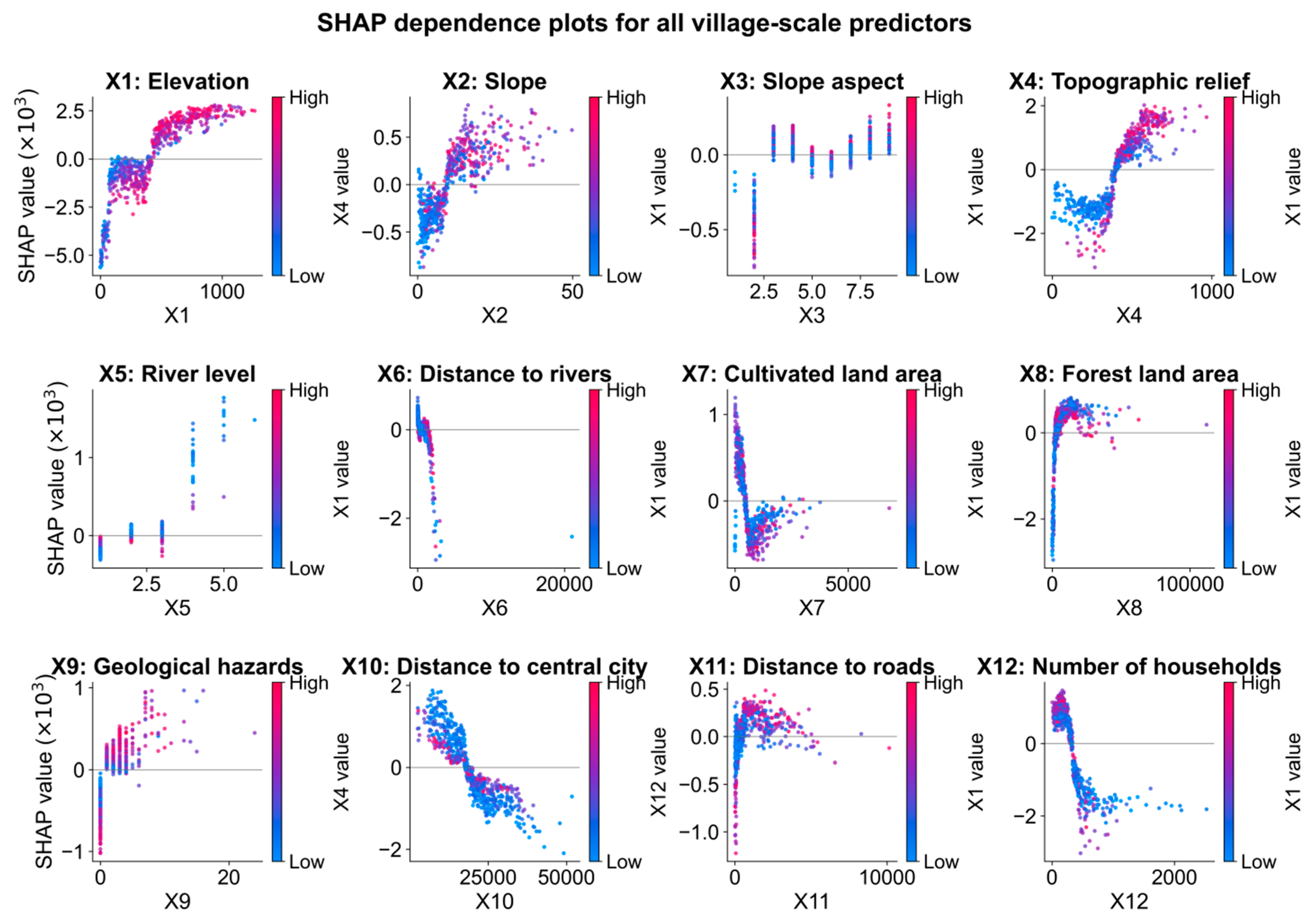
SHAP dependence plots for all X1–X12 village-scale predictors. Vertical position is the feature-specific SHAP contribution multiplied by 103, and each panel’s right-hand colour bar identifies the value of that predictor’s strongest interacting feature. Patterns are predictive and exploratory rather than causal.
Figure 7.
SHAP dependence plots for all X1–X12 village-scale predictors. Vertical position is the feature-specific SHAP contribution multiplied by 103, and each panel’s right-hand colour bar identifies the value of that predictor’s strongest interacting feature. Patterns are predictive and exploratory rather than causal.
Figure 8.
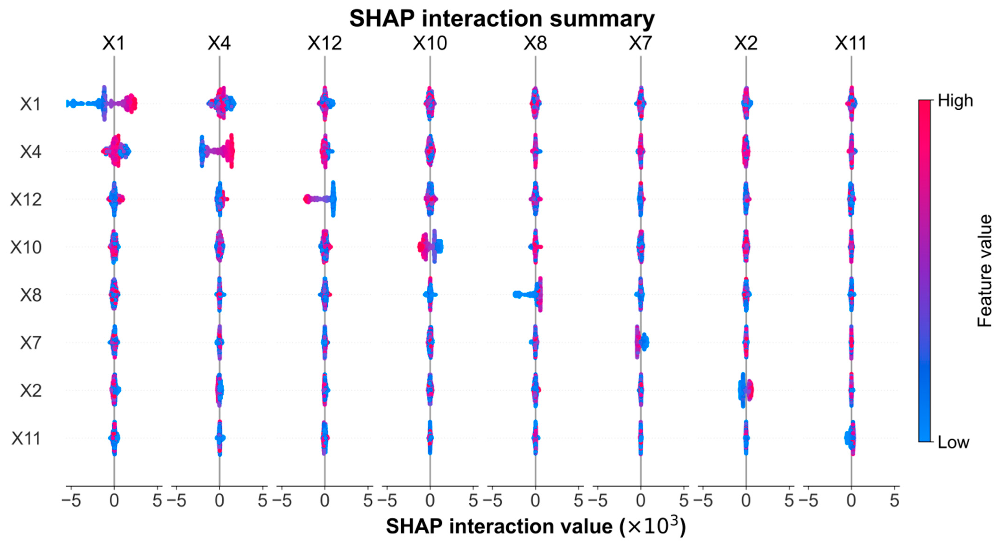
SHAP interaction summary for the eight leading predictors in the final X1–X12 Random Forest. Rows and columns identify feature pairs, horizontal position represents the pairwise interaction contribution multiplied by 103, and the common blue–purple–magenta scale denotes low-to-high feature values.
Figure 8.
SHAP interaction summary for the eight leading predictors in the final X1–X12 Random Forest. Rows and columns identify feature pairs, horizontal position represents the pairwise interaction contribution multiplied by 103, and the common blue–purple–magenta scale denotes low-to-high feature values.
Figure 9.
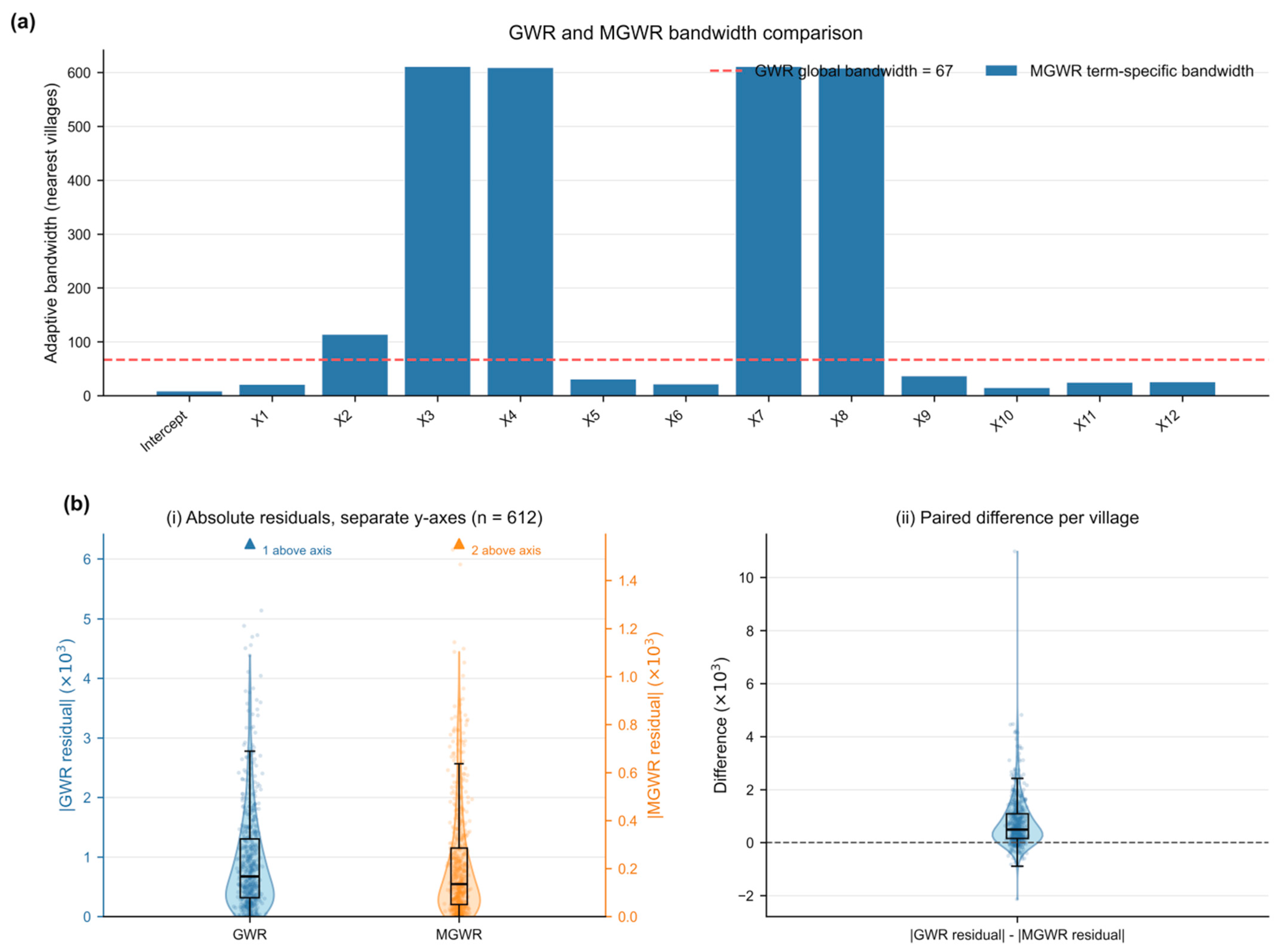
GWR-MGWR bandwidth and residual comparison. (a) AICc-selected adaptive nearest-neighbour bandwidths: GWR used a single 67-neighbour bandwidth, whereas MGWR selected term-specific bandwidths from nine to 611 neighbours. (b-i) Violin and box plots of absolute GWR and MGWR residuals, displayed on separate labelled y-axes because their numerical ranges differ; GWR is read against the left axis and MGWR against the right axis. For legibility, the violin density outlines end at the 99th percentile, and the axis limits place this percentile at approximately 70% of the panel height. Box-plot statistics use all 612 observations; one GWR and two MGWR observations beyond the displayed limits are identified by triangles at the top of the respective axes. (b-ii) Paired village-level differences defined as |GWR residual| minus |MGWR residual|. Positive values indicate smaller absolute residuals under MGWR.
Figure 9.
GWR-MGWR bandwidth and residual comparison. (a) AICc-selected adaptive nearest-neighbour bandwidths: GWR used a single 67-neighbour bandwidth, whereas MGWR selected term-specific bandwidths from nine to 611 neighbours. (b-i) Violin and box plots of absolute GWR and MGWR residuals, displayed on separate labelled y-axes because their numerical ranges differ; GWR is read against the left axis and MGWR against the right axis. For legibility, the violin density outlines end at the 99th percentile, and the axis limits place this percentile at approximately 70% of the panel height. Box-plot statistics use all 612 observations; one GWR and two MGWR observations beyond the displayed limits are identified by triangles at the top of the respective axes. (b-ii) Paired village-level differences defined as |GWR residual| minus |MGWR residual|. Positive values indicate smaller absolute residuals under MGWR.
Figure 10.
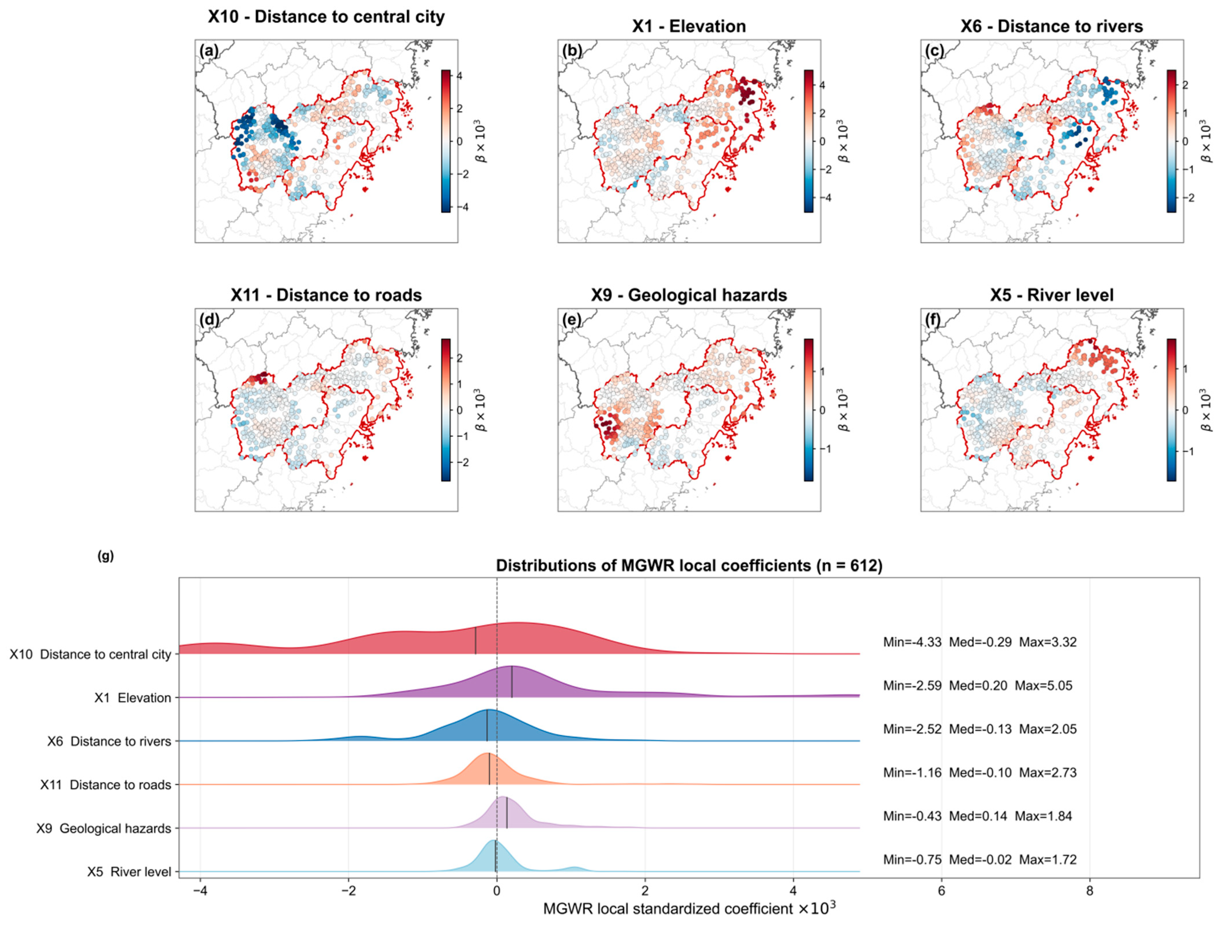
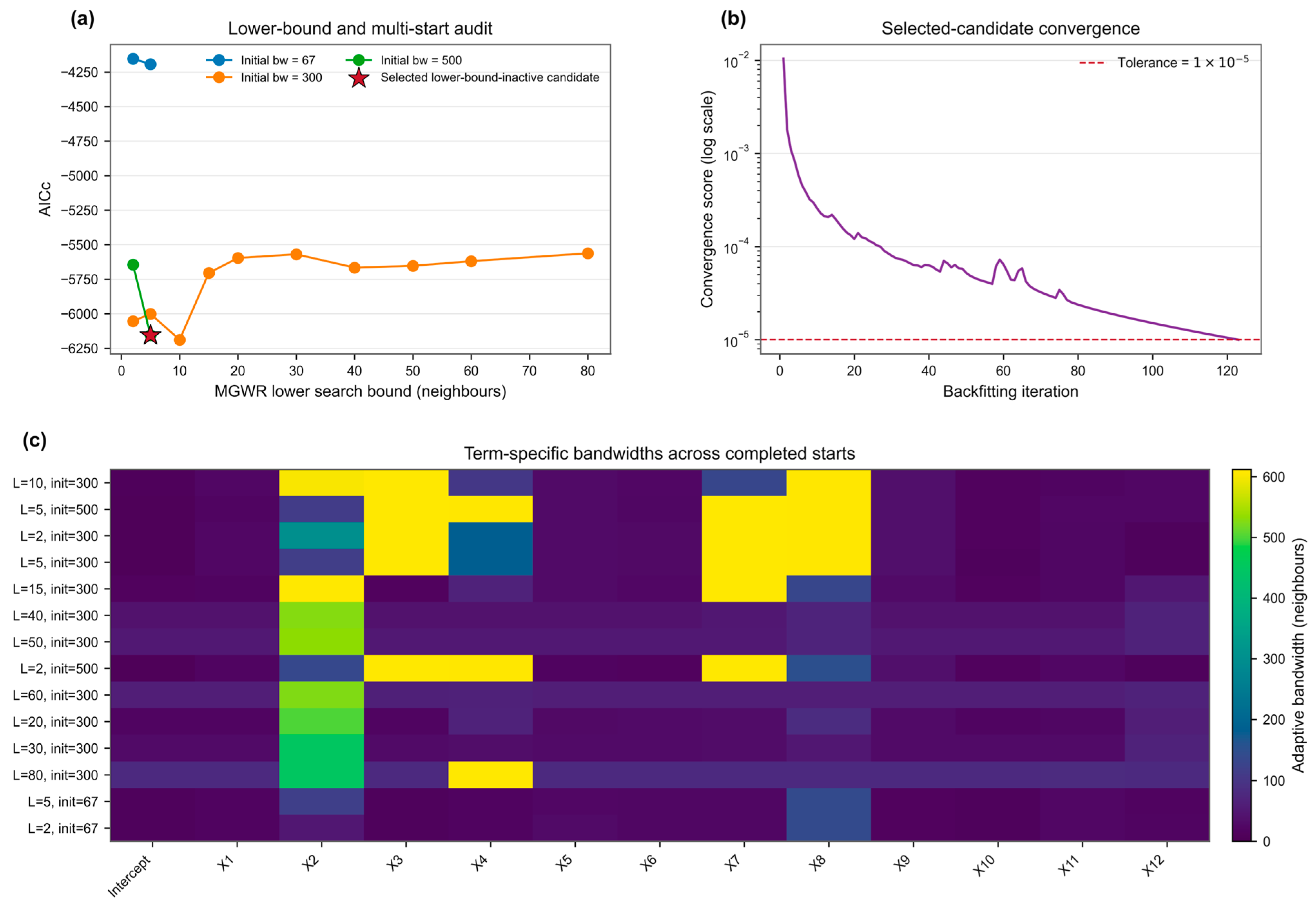
MGWR local standardized coefficient results for the six X1–X12 terms with the largest local variation in the revised primary lower-bound-inactive candidate. (a–f) Framed coefficient maps over the study area and surrounding province, city, and county boundaries; (g) ridgeline distributions summarizing each mapped coefficient surface. Coefficients are multiplied by 103 for legibility only. Multi-start sensitivity, small local bandwidths, near-global upper-bound terms, and elevated local conditioning require exploratory interpretation.
Figure 10.
MGWR local standardized coefficient results for the six X1–X12 terms with the largest local variation in the revised primary lower-bound-inactive candidate. (a–f) Framed coefficient maps over the study area and surrounding province, city, and county boundaries; (g) ridgeline distributions summarizing each mapped coefficient surface. Coefficients are multiplied by 103 for legibility only. Multi-start sensitivity, small local bandwidths, near-global upper-bound terms, and elevated local conditioning require exploratory interpretation.
Figure 11.
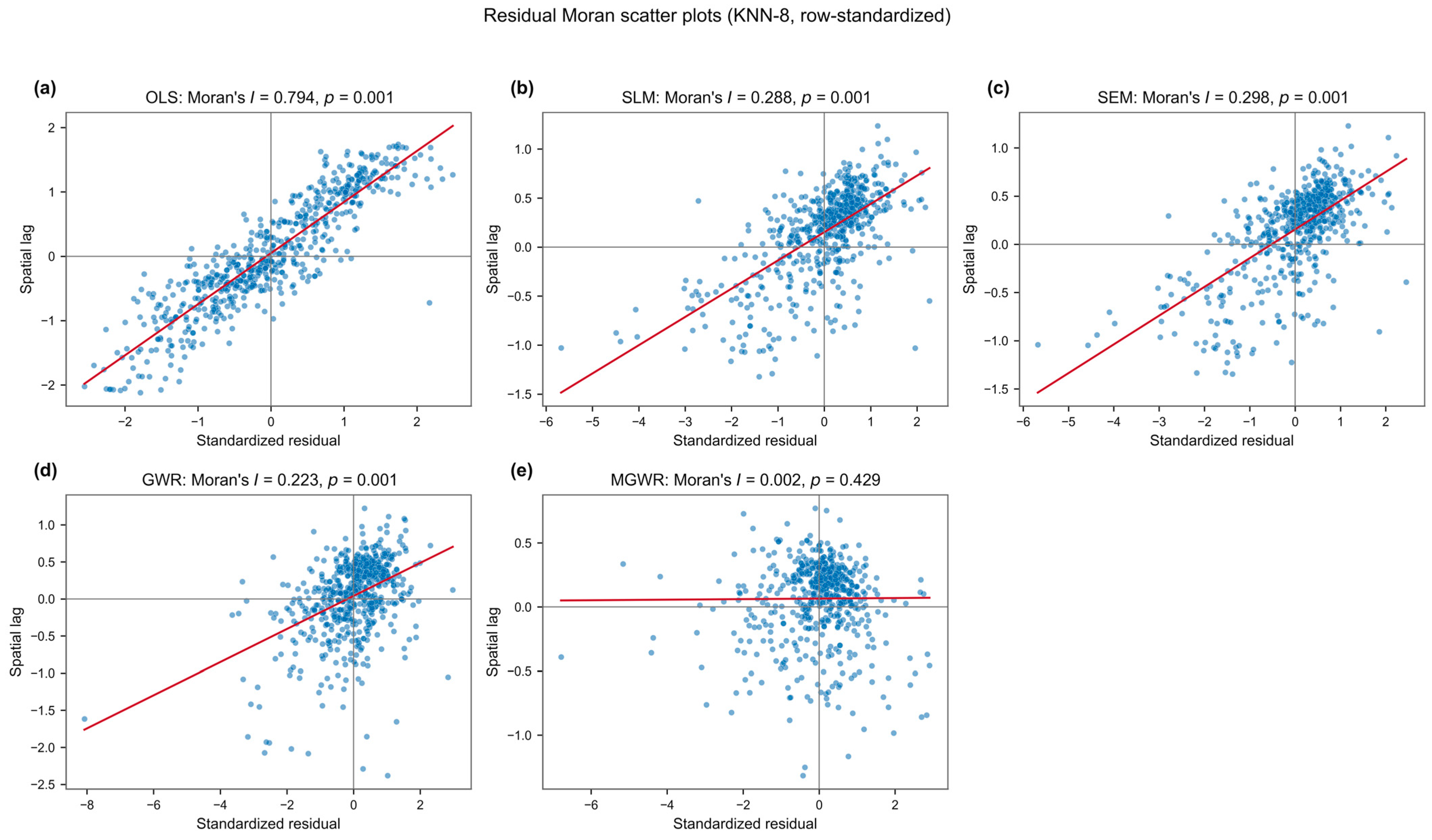
Moran scatter plots for model-native residuals or innovations: (a) OLS residuals; (b) SLM structural disturbances; (c) SEM filtered innovations; (d) GWR residuals; and (e) MGWR residuals. All panels use row-standardized KNN-8 weights; Moran’s I and permutation p-values are reported in each panel.
Figure 11.
Moran scatter plots for model-native residuals or innovations: (a) OLS residuals; (b) SLM structural disturbances; (c) SEM filtered innovations; (d) GWR residuals; and (e) MGWR residuals. All panels use row-standardized KNN-8 weights; Moran’s I and permutation p-values are reported in each panel.
Figure 12.
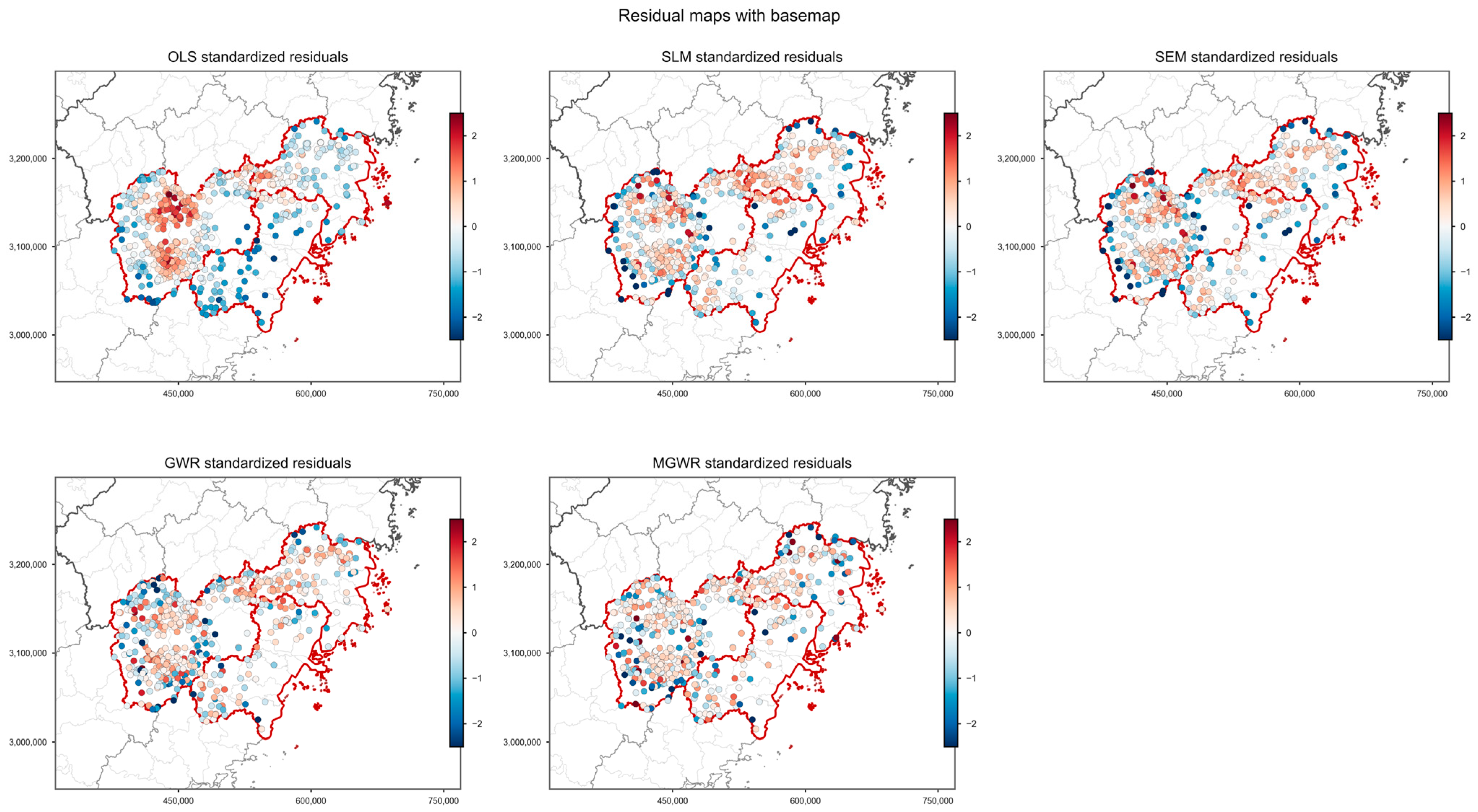
Framed small-multiple maps of standardized model-native residuals or innovations for OLS, SLM, SEM, GWR, and MGWR. A shared diverging scale permits direct visual comparison, and the contextual administrative boundaries are retained.
Figure 12.
Framed small-multiple maps of standardized model-native residuals or innovations for OLS, SLM, SEM, GWR, and MGWR. A shared diverging scale permits direct visual comparison, and the contextual administrative boundaries are retained.
Figure 13.
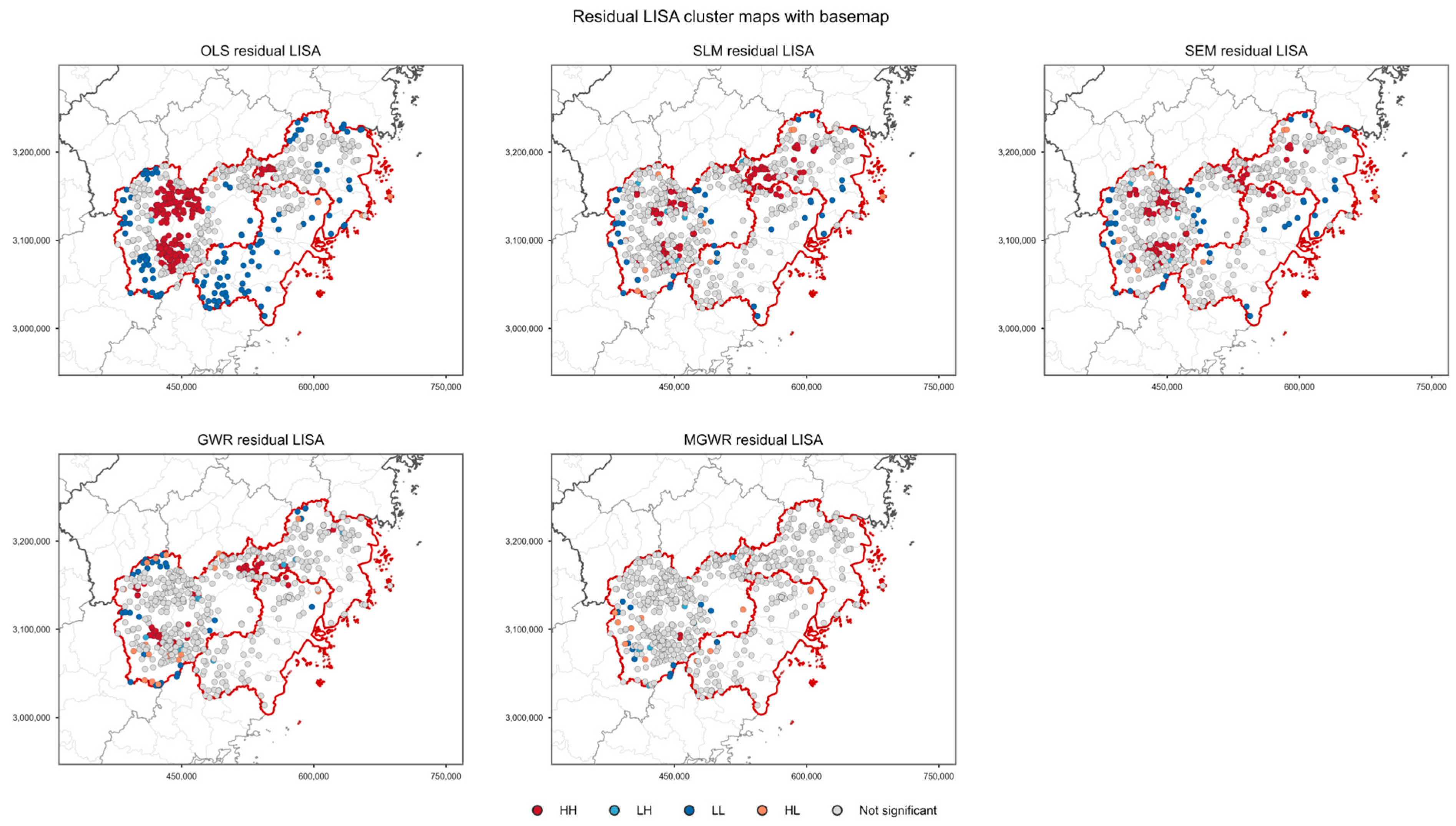
Framed LISA cluster maps for model-native residuals or innovations (p < 0.05; 999 permutations; row-standardized KNN-8 weights). A common legend is used across all panels.
Figure 13.
Framed LISA cluster maps for model-native residuals or innovations (p < 0.05; 999 permutations; row-standardized KNN-8 weights). A common legend is used across all panels.
Figure 14.
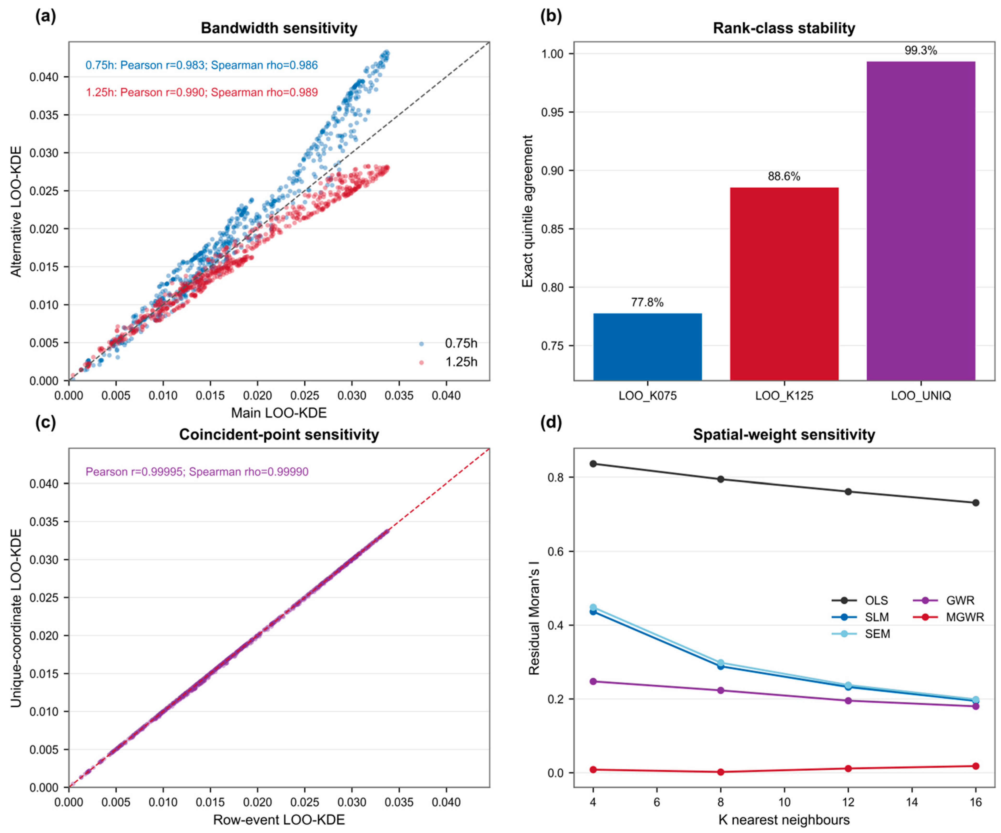
LOO-KDE and residual-spatial-dependence sensitivity: (a) distributions under 0.75 h, the main bandwidth h, and 1.25 h; (b) rank and quintile agreement; (c) influence of treating coincident coordinates as unique spatial events; and (d) residual Moran’s I under KNN values of 4, 8, 12, and 16.
Figure 14.
LOO-KDE and residual-spatial-dependence sensitivity: (a) distributions under 0.75 h, the main bandwidth h, and 1.25 h; (b) rank and quintile agreement; (c) influence of treating coincident coordinates as unique spatial events; and (d) residual Moran’s I under KNN values of 4, 8, 12, and 16.
Figure 15.
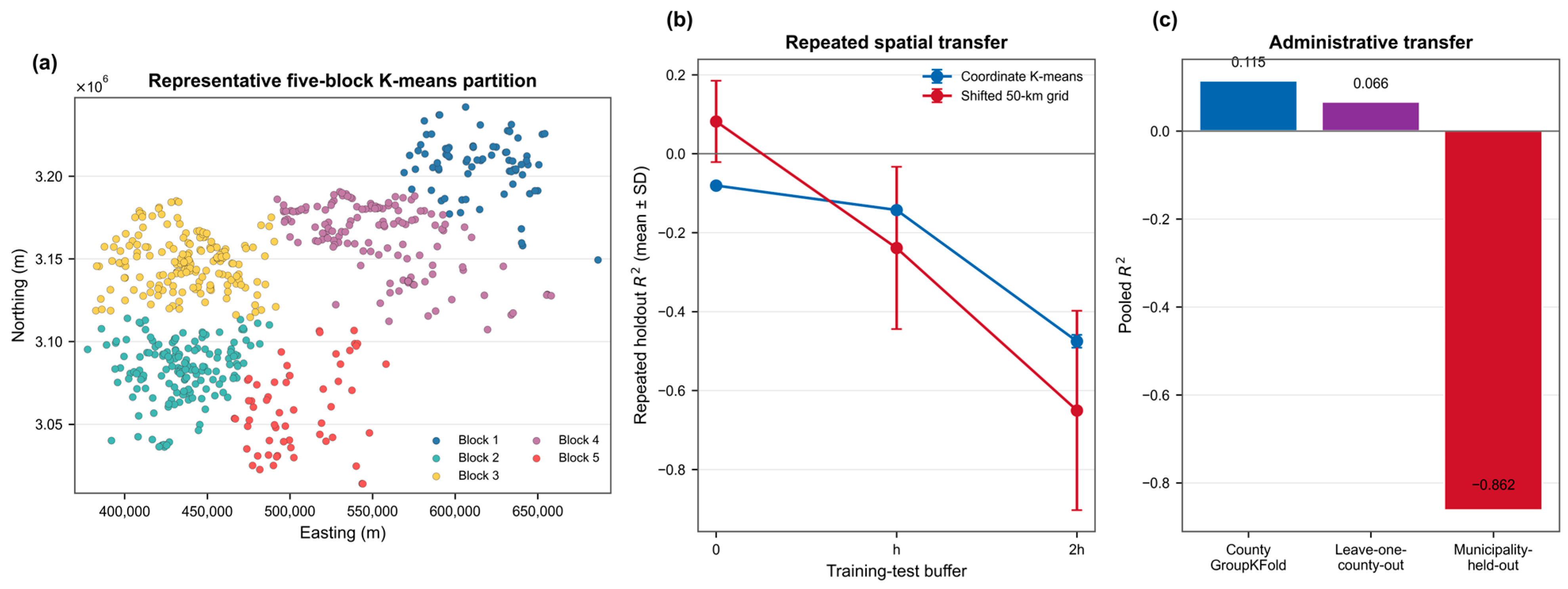
Geographic-transfer validation at increasing separation. (a) Representative coordinate K-means partition displayed in the original EPSG:4549 projected coordinates with an equal map aspect ratio; (b) mean ± standard deviation across 30 coordinate K-means and 30 shifted 50 km grid holdouts under no buffer, a one-bandwidth buffer (h), and a two-bandwidth buffer (2 h); and (c) county- and municipality-held-out transfer. Negative R2 values indicate performance below an intercept-only prediction for the held-out observations.
Figure 15.
Geographic-transfer validation at increasing separation. (a) Representative coordinate K-means partition displayed in the original EPSG:4549 projected coordinates with an equal map aspect ratio; (b) mean ± standard deviation across 30 coordinate K-means and 30 shifted 50 km grid holdouts under no buffer, a one-bandwidth buffer (h), and a two-bandwidth buffer (2 h); and (c) county- and municipality-held-out transfer. Negative R2 values indicate performance below an intercept-only prediction for the held-out observations.
Figure 16.
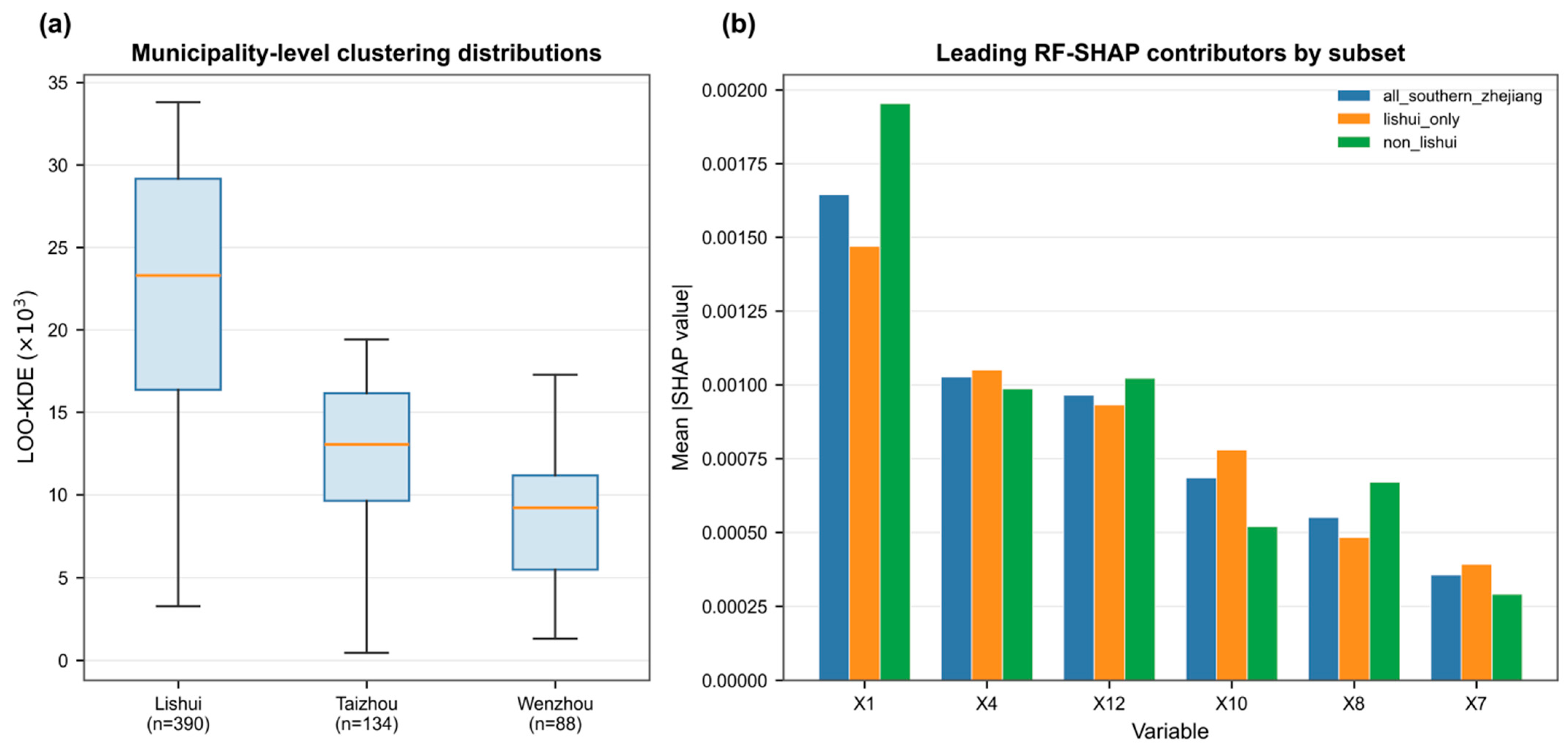
Municipality and geographic-subset comparison. (a) Box plots of LOO-KDE distributions in Lishui, Taizhou, and Wenzhou. (b) Mean absolute RF-SHAP contributions of the six leading full-region predictors, summarized for all southern Zhejiang villages, the Lishui subset, and the non-Lishui subset. These are within-model descriptive subgroup summaries rather than separately refitted models.
Figure 16.
Municipality and geographic-subset comparison. (a) Box plots of LOO-KDE distributions in Lishui, Taizhou, and Wenzhou. (b) Mean absolute RF-SHAP contributions of the six leading full-region predictors, summarized for all southern Zhejiang villages, the Lishui subset, and the non-Lishui subset. These are within-model descriptive subgroup summaries rather than separately refitted models.
Table 1.
Dependent variable and explanatory variables for traditional villages in southern Zhejiang, with units, spatial scales, and data sources: (N) natural geographic factors; (S) socio-economic factors.
Table 1.
Dependent variable and explanatory variables for traditional villages in southern Zhejiang, with units, spatial scales, and data sources: (N) natural geographic factors; (S) socio-economic factors.
| Code | Variable | Definition/Calculation | Unit | Spatial Scale | Data Source | Reference Year |
|---|
| Y | LOO-KDE local clustering intensity | Gaussian leave-one-out KDE calculated from all other recognized villages; focal village excluded | villages km−2 | village point | Recognized-village inventory; authors’ Python/GIS calculation | Inventory to 2023 |
| X1 | Elevation | DEM elevation extracted at the village centroid | m | village point | ASTER GDEM 30 m, RESDC | Terrain invariant |
| X2 | Slope | Slope derived from DEM at village centroid | degree | village point | ASTER GDEM 30 m; authors’ GIS calculation | Terrain invariant |
| X3 | Slope aspect | Aspect azimuth derived from DEM | degree (0–360) | village point | ASTER GDEM 30 m; authors’ GIS calculation | Terrain invariant |
| X4 | Topographic relief | Maximum–minimum elevation difference within local terrain window | m | local terrain window | ASTER GDEM 30 m; authors’ GIS calculation | Terrain invariant |
| X5 | River level | Order/grade of the nearest mapped river | ordinal grade | nearest river feature | RESDC water-body/river data; authors’ extraction | 2023-aligned |
| X6 | Distance to rivers | Euclidean distance from village centroid to nearest mapped river | m | village point | RESDC water data; authors’ GIS calculation | 2023-aligned |
| X7 | Cultivated land area | Registered cultivated land area associated with the village | mu (1 mu = 1/15 ha = 666.7 m2) | village unit | Field investigation and local government statistics | 2023 |
| X8 | Forest land area | Registered forest land area associated with the village | mu | village unit | Field investigation and local government statistics | 2023 |
| X9 | Geological hazards | Recorded geological-hazard events within 3 km of the village | count | 3 km village buffer | RESDC geological-hazard records; authors’ GIS calculation | records to 2023 |
| X10 | Distance to the central city | Euclidean distance from village to nearest designated central-city coordinate | m | village point | Compiled city coordinates; authors’ GIS calculation | 2023-aligned |
| X11 | Distance to roads | Euclidean distance to the nearest road in the analysis network | m | village point | National 1:250,000 road network; authors’ GIS calculation | 2023 |
| X12 | Number of households | Registered households in the village | households | village unit | Authors’ field survey and village records | 2024 records; surveyed 2025 |
| X13 | GDP | Total GDP of the county-level administrative unit | 10,000 CNY | county/district context | Taizhou, Wenzhou, and Lishui statistical yearbooks | 2023 |
| X14 | Per capita GDP | County/district GDP per resident | CNY/person | county/district context | Municipal statistical yearbooks | 2023 |
| X15 | Rural per capita disposable income | County/district rural disposable income per resident | CNY/person | county/district context | Municipal statistical yearbooks | 2023 |
| X16 | Primary industry output | Gross output value of the primary industry | 10,000 CNY | county/district context | Municipal statistical yearbooks | 2023 |
| X17 | Secondary industry output | Gross output value of the secondary industry | 10,000 CNY | county/district context | Municipal statistical yearbooks | 2023 |
| X18 | Tertiary industry output | Gross output value of the tertiary industry | 10,000 CNY | county/district context | Municipal statistical yearbooks | 2023 |
Table 2.
Correlation-screening decision and VIF results for the final X1–X12 village-scale predictor set.
Table 2.
Correlation-screening decision and VIF results for the final X1–X12 village-scale predictor set.
| Variable | VIF | Tolerance | Decision |
|---|
| X1 | 1.727 | 0.579 | Retained |
| X2 | 1.407 | 0.711 | Retained |
| X3 | 1.032 | 0.969 | Retained |
| X4 | 1.963 | 0.509 | Retained |
| X5 | 1.169 | 0.855 | Retained |
| X6 | 1.067 | 0.937 | Retained |
| X7 | 1.528 | 0.654 | Retained |
| X8 | 1.378 | 0.726 | Retained |
| X9 | 1.029 | 0.972 | Retained |
| X10 | 1.134 | 0.882 | Retained |
| X11 | 1.189 | 0.841 | Retained |
| X12 | 1.543 | 0.648 | Retained |
Table 3.
OLS, SLM, and SEM coefficients for standardized X1–X12 predictors on the original LOO-KDE scale. SLM/SEM spatial parameters are reported as rho and lambda; KNN-8 weights are row-standardized.
Table 3.
OLS, SLM, and SEM coefficients for standardized X1–X12 predictors on the original LOO-KDE scale. SLM/SEM spatial parameters are reported as rho and lambda; KNN-8 weights are row-standardized.
| Term | OLS Beta | OLS p | SLM Beta | SLM p | SEM Beta | SEM p |
|---|
| Intercept | 0.018250 | 1.07 × 10−265 | −1.93 × 10⁻⁴ | 3.49 × 10⁻⁴ | −0.022640 | 3.46 × 10⁻⁷ |
| X1 | 0.003146 | 1.11 × 10⁻¹⁵ | 1.56 × 10⁻⁴ | 0.0191 | 1.78 × 10⁻⁴ | 0.0642 |
| X2 | 1.14 × 10⁻⁴ | 0.7419 | 1.12 × 10⁻⁵ | 0.8498 | 1.53 × 10⁻⁵ | 0.7832 |
| X3 | 4.21 × 10⁻⁴ | 0.1540 | 3.45 × 10⁻⁵ | 0.4935 | 1.12 × 10⁻⁶ | 0.9820 |
| X4 | 0.001707 | 3.19 × 10⁻⁵ | 1.08 × 10⁻⁴ | 0.1216 | 6.10 × 10⁻⁵ | 0.3995 |
| X5 | 0.001652 | 2.06 × 10⁻⁷ | 5.00 × 10⁻⁵ | 0.3531 | 3.13 × 10⁻⁵ | 0.5904 |
| X6 | −9.11 × 10⁻⁴ | 0.0025 | −9.80 × 10⁻⁵ | 0.0562 | −1.17 × 10⁻⁴ | 0.0429 |
| X7 | −6.36 × 10⁻⁵ | 0.8595 | −7.81 × 10⁻⁶ | 0.8989 | 2.47 × 10⁻⁵ | 0.7064 |
| X8 | 5.38 × 10⁻⁵ | 0.8747 | −2.21 × 10⁻⁵ | 0.7048 | 5.65 × 10⁻⁵ | 0.3600 |
| X9 | 1.97 × 10⁻⁴ | 0.5038 | 3.71 × 10⁻⁵ | 0.4625 | 4.79 × 10⁻⁵ | 0.3883 |
| X10 | −0.002135 | 1.34 × 10⁻¹¹ | −1.82 × 10⁻⁴ | 7.45 × 10⁻⁴ | −2.65 × 10⁻⁴ | 0.0241 |
| X11 | −2.47 × 10⁻⁴ | 0.4355 | −1.67 × 10⁻⁴ | 0.0021 | −1.25 × 10⁻⁴ | 0.0325 |
| X12 | −0.001062 | 0.0034 | 4.83 × 10⁻⁶ | 0.9378 | −1.10 × 10⁻⁵ | 0.8703 |
| rho | - | - | 0.984637 | 0.0000 | - | - |
| lambda | - | - | - | - | 0.988723 | 0.0000 |
Table 4.
Definition-audited model fit. SLM structural and SEM filtered rows are in-sample model-native diagnostics; SLM reduced-form and SEM systematic rows are covariate-based predictions. Package pseudo-R2 values are not directly comparable across definitions.
Table 4.
Definition-audited model fit. SLM structural and SEM filtered rows are in-sample model-native diagnostics; SLM reduced-form and SEM systematic rows are covariate-based predictions. Package pseudo-R2 values are not directly comparable across definitions.
| Model/Metric | Definition | R2 | RMSE | MAE | Package R2/Pseudo-R2 | AIC or AICc |
|---|
| OLS | response-scale fitted value X beta | 0.3047 | 0.007113 | 0.005871 | - | −4290.97 |
| SLM structural fit | rho W y + X beta | 0.9792 | 0.001229 | 8.93 × 10⁻⁴ | 0.9803 | −6266.48 |
| SLM reduced form | (I − rho W)−1 X beta | −9.8195 | 0.028057 | 0.026555 | 0.9803 | −6266.48 |
| SEM systematic | X beta | −22.9488 | 0.041743 | 0.040889 | 0.1615 | −6256.19 |
| SEM filtered fit | y minus filtered innovation | 0.9791 | 0.001233 | 8.88 × 10⁻⁴ | 0.1615 | −6256.19 |
| GWR | response fitted value | 0.9743 | 0.001368 | 9.59 × 10⁻⁴ | 0.9743 | −5463.77 |
| MGWR | response fitted value | 0.9984 | 0.000341 | 2.22 × 10⁻⁴ | 0.9984 | −6155.20 |
Table 5.
Residual global Moran’s I and significant LISA cluster counts for the final X1–X12 models (row-standardized KNN-8 weights; 999 permutations).
Table 5.
Residual global Moran’s I and significant LISA cluster counts for the final X1–X12 models (row-standardized KNN-8 weights; 999 permutations).
| Model | Residual Moran’s I | z (Permutation) | p (Permutation) | Significant LISA n | HH/LL/HL/LH |
|---|
| OLS | 0.7943 | 42.62 | 0.001 | 328 | 188/133/4/3 |
| SLM | 0.2882 | 15.59 | 0.001 | 156 | 96/44/9/7 |
| SEM | 0.2980 | 15.96 | 0.001 | 172 | 111/48/8/5 |
| GWR | 0.2231 | 11.53 | 0.001 | 124 | 53/39/20/12 |
| MGWR | 0.0021 | 0.19 | 0.429 | 38 | 2/12/14/10 |
Table 6.
RF tuning, administrative transfer, and repeated spatially grouped holdout results for X1–X12. Spatial rows report means across 30 repetitions.
Table 6.
RF tuning, administrative transfer, and repeated spatially grouped holdout results for X1–X12. Spatial rows report means across 30 repetitions.
| Validation Design | Predictors | R2 | RMSE | MAE | Interpretation |
|---|
| apparent_training | X1–X12 | 0.5762 | 0.005553 | 0.004564 | diagnostic/grouped estimate |
| out_of_bag | X1–X12 | 0.3531 | 0.006861 | 0.005656 | diagnostic/grouped estimate |
| county_GroupKFold_pooled | X1–X12 | 0.1147 | 0.008026 | 0.006663 | diagnostic/grouped estimate |
| leave_one_county_out | X1–X12 | 0.0664 | 0.008224 | 0.006804 | administrative transfer |
| municipality_held_out | X1–X12 | −0.8620 | 0.011639 | 0.009719 | administrative transfer |
| coordinate_kmeans; buffer 0 | X1–X12 | −0.0807 | 0.008867 | 0.007483 | mean of 30 repetitions |
| coordinate_kmeans; buffer h | X1–X12 | −0.1426 | 0.009118 | 0.007681 | mean of 30 repetitions |
| coordinate_kmeans; buffer 2 h | X1–X12 | −0.4753 | 0.010360 | 0.008631 | mean of 30 repetitions |
| shifted_50 km_grid; buffer 0 | X1–X12 | 0.0818 | 0.008162 | 0.006770 | mean of 30 repetitions |
| shifted_50 km_grid; buffer h | X1–X12 | −0.2388 | 0.009463 | 0.007768 | mean of 30 repetitions |
| shifted_50 km_grid; buffer 2 h | X1–X12 | −0.6503 | 0.010914 | 0.008997 | mean of 30 repetitions |
Table 7.
AICc-selected GWR/MGWR adaptive bandwidths and MGWR local coefficient variability for the X1–X12 specification.
Table 7.
AICc-selected GWR/MGWR adaptive bandwidths and MGWR local coefficient variability for the X1–X12 specification.
| Term | GWR Bandwidth | MGWR Bandwidth | MGWR Mean Beta | Local Beta SD | Local Beta Range |
|---|
| Intercept | 67 | 9 | 0.019326 | 0.007057 | 0.00403 to 0.03148 |
| X1 | 67 | 21 | 5.85 × 10⁻⁴ | 0.001360 | −0.00259 to 0.00505 |
| X2 | 67 | 114 | 2.14 × 10⁻⁵ | 6.98 × 10⁻⁵ | −2.01 × 10⁻⁴ to 1.87 × 10⁻⁴ |
| X3 | 67 | 611 | −5.60 × 10⁻⁵ | 5.71 × 10⁻⁶ | −6.85 × 10⁻⁵ to −4.94 × 10⁻⁵ |
| X4 | 67 | 609 | −1.70 × 10⁻⁵ | 6.81 × 10⁻⁶ | −2.99 × 10⁻⁵ to −6.61 × 10⁻⁶ |
| X5 | 67 | 31 | 5.54 × 10⁻⁵ | 3.68 × 10⁻⁴ | −7.50 × 10⁻⁴ to 0.00172 |
| X6 | 67 | 22 | −1.89 × 10⁻⁴ | 7.27 × 10⁻⁴ | −0.00252 to 0.00205 |
| X7 | 67 | 611 | −5.14 × 10⁻⁵ | 3.52 × 10⁻⁶ | −5.64 × 10⁻⁵ to −4.57 × 10⁻⁵ |
| X8 | 67 | 608 | 1.03 × 10⁻⁵ | 1.50 × 10⁻⁵ | −5.18 × 10⁻⁶ to 3.89 × 10⁻⁵ |
| X9 | 67 | 37 | 2.21 × 10⁻⁴ | 3.86 × 10⁻⁴ | −4.28 × 10⁻⁴ to 0.00184 |
| X10 | 67 | 15 | −6.95 × 10⁻⁴ | 0.001653 | −0.00433 to 0.00332 |
| X11 | 67 | 25 | −3.24 × 10⁻⁵ | 4.79 × 10⁻⁴ | −0.00116 to 0.00273 |
| X12 | 67 | 26 | 1.30 × 10⁻⁴ | 3.64 × 10⁻⁴ | −6.49 × 10⁻⁴ to 0.00246 |




 ,
,