Quasi-Experimental Evaluation of the Association Between Payments for Ecosystem Services and Satellite-Based Vegetation Dynamics in Cundinamarca, Colombia

Abstract

Payments for Ecosystem Services (PES) are increasingly used to promote conservation, but evidence of their biophysical outcomes remains mixed because participation is rarely assigned at random. This study assessed the association between participation in the Yo Protejo ¡Agua para Todos! PES program and satellite-based vegetation dynamics in Cundinamarca, Colombia, during 2015–2024. Annual NDVI, EVI, and SAVI values were derived from Landsat 8 and 9 imagery processed in Google Earth Engine. The empirical strategy combined fixed-effects difference-in-differences models, two spatial comparison groups, propensity-score adjustment, inverse probability of treatment weighting, property-clustered inference, event-study diagnostics, differential-trend models, and property-year robustness analyses. Pre-treatment and covariate-balance diagnostics indicated imperfect counterfactual comparability, particularly for the external 500–1000 m buffer-ring controls. No vegetation index produced uniformly positive and robust associations across specifications. NDVI showed a small positive association during program implementation under the 500 m neighboring-control definition, but this result was not preserved after differential-trend adjustment or property-year aggregation. EVI produced positive point-level estimates under the external control, although this specification retained substantial residual imbalance and the estimates became negative after property-year aggregation. SAVI provided no robust positive evidence and showed negative post-implementation differentials in some external-control models. Overall, the estimated associations were sensitive to the vegetation metric, comparison-group definition, temporal phase, inferential level, and spatial aggregation. The results should therefore be interpreted as specification-dependent adjusted associations rather than definitive causal effects.

1. Introduction

Payments for Ecosystem Services (PES) are voluntary and conditional economic transfers intended to align individual land-use decisions with collective objectives such as water regulation, carbon sequestration, biodiversity conservation, and soil protection [1]. In practice, PES rarely operate as pure market exchanges. They generally function as mixed institutional arrangements involving public agencies, communities, non-governmental organizations, and private actors under conditions of territorial targeting, monitoring constraints, and overlapping conservation and rural-development objectives [2,3,4].

Although PES have expanded worldwide [5], their adoption does not guarantee measurable environmental outcomes. Program performance depends on spatial targeting, contract duration, incentive intensity, conditionality, monitoring, and enforcement capacity [4,6,7,8]. Moreover, participating areas are rarely selected at random; they are often prioritized because of their ecological importance, degradation history, or exposure to environmental threats. Consequently, administrative indicators or simple before-and-after comparisons may provide misleading evidence when treated areas differ systematically from untreated locations [4,9,10,11].

Empirical findings remain heterogeneous. Some programs have reduced deforestation or improved conservation outcomes when incentives were targeted toward areas under substantial pressure and maintained long enough to influence land-use decisions, as reported in Uganda and Mexico [12,13]. Other studies show that effectiveness can improve through better beneficiary selection, contract design, and treatment targeting [8]. However, broader reviews find that many programs generate modest, null, or ambiguous outcomes, particularly where transformation pressure is low, targeting is weak, or monitoring and enforcement are limited [4,14].

In Colombia, PES are formally regulated under Decree-Law 870 of 2017 [15]. Cundinamarca has implemented several initiatives aimed at conserving ecosystems associated with water regulation and provision, including the Yo Protejo ¡Agua para Todos! program [16]. However, enrolled area, financial execution, and beneficiary counts do not establish whether participation is associated with measurable ecological outcomes. Rigorous evidence on the biophysical performance of subnational PES programs in Colombia therefore remains limited.

This study evaluates satellite-based vegetation dynamics associated with participation in Yo Protejo ¡Agua para Todos! during 2015–2024. Vegetation condition is assessed using Landsat-derived NDVI, EVI, and SAVI, which differ in their sensitivity to canopy density, atmospheric effects, and soil background [17,18,19]. The empirical strategy compares treated areas with a neighboring 500 m control and an external 500–1000 m buffer-ring control. It combines fixed-effects difference-in-differences models, propensity-score weighting, property-clustered inference, placebo and event-study diagnostics, differential-trend specifications, property-year aggregation, and restricted pre-treatment-comparable samples.

The objective is to assess how vegetation dynamics differ between PES-treated and comparable untreated areas and whether the estimated associations vary across vegetation indices, spatial counterfactuals, temporal phases, inferential levels, and analytical specifications. The study contributes by integrating three complementary vegetation metrics, two alternative spatial comparison groups, and multiple robustness strategies within a unified quasi-experimental framework. Rather than proposing a new estimator, it provides a transparent design for examining how evaluations of conservation-incentive programs depend on spectral measurement, counterfactual construction, spatial aggregation, and statistical inference.

2. Materials and Methods

2.1. Study Area and Treatment Definition, and Spatial Comparison Groups

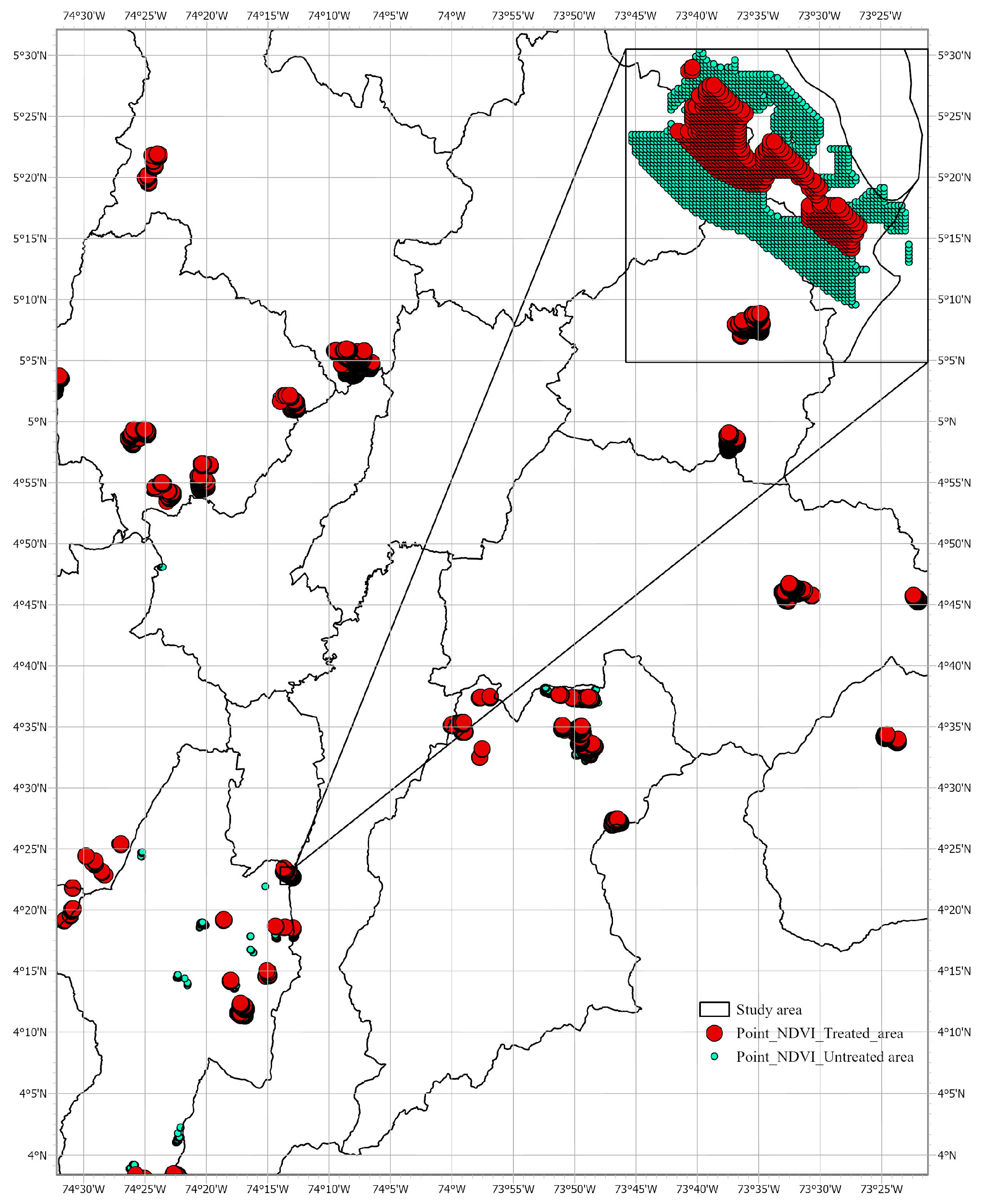
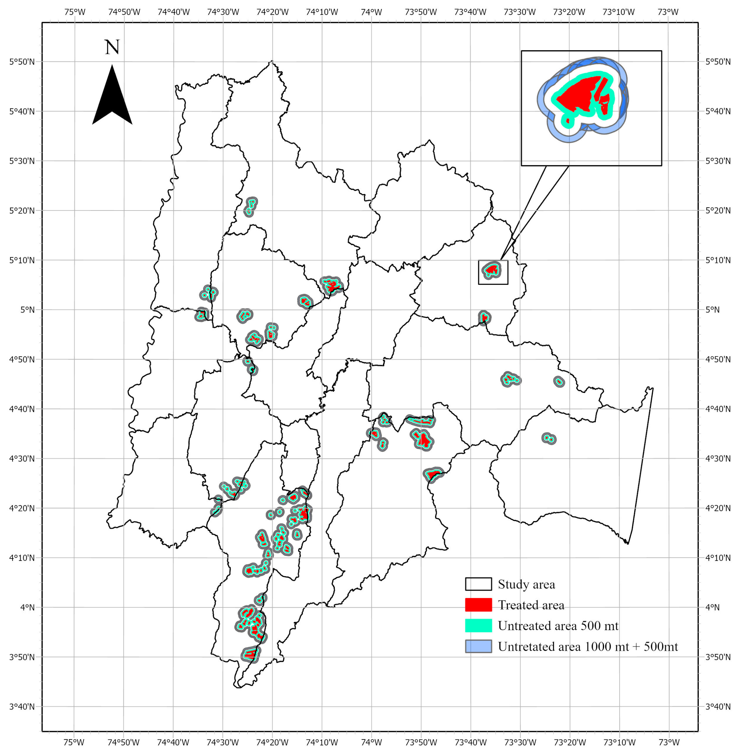
The study was conducted in the department of Cundinamarca, Colombia, in areas associated with the Payments for Ecosystem Services (PES) program Yo Protejo ¡Agua para Todos!, a water-related conservation initiative aimed at protecting strategic ecosystems linked to water regulation and provision. The treated areas corresponded to the polygons or properties enrolled in the PES program (Figure 1). These areas were used as the spatial basis for defining the treatment group and for constructing alternative comparison groups. All treated properties entered the PES program in 2018 and remained enrolled until the end of 2020. Treatment adoption was therefore simultaneous across properties rather than staggered over time.

Because participation in the PES program was not randomly assigned, two spatial comparison groups were constructed. The first comparison group consisted of untreated areas located within a 500 m buffer around the perimeter of the treated polygons, excluding all areas enrolled in the PES program. This comparison group allowed treated areas to be compared with nearby untreated areas expected to share broadly similar local biophysical and agroclimatic conditions, following the use of surrounding or buffer areas in spatial evaluations of conservation interventions [20,21,22].

A second comparison group was constructed as an external buffer-ring control. In this specification, the first 500 m surrounding the treated polygons were excluded as a separation band, and the subsequent 500 m ring was used as an alternative comparison area. Thus, this second control group corresponded to untreated areas located approximately between 500 m and 1000 m from the boundary of the PES-treated polygons. This design was included to reduce potential contamination from immediately adjacent areas, such as local spillovers, shared management practices, or direct spatial dependence between treated and neighboring untreated areas. However, increasing spatial separation may also reduce environmental and observable comparability. The use of alternative comparison areas is consistent with recommendations emphasizing the importance of constructing credible counterfactuals in conservation impact evaluations [9,10,11,21,22]. Therefore, all analyses were implemented separately for two control definitions: the 500 m neighboring-control group and the external 500–1000 m buffer-ring control group.

The units of analysis corresponded to spatial observation points derived from valid Landsat pixels located within treated and comparison polygons. Each point represented a valid 30 m Landsat pixel and was spatially associated with its corresponding property, municipality, PES modality, and comparison group. The PES modality distinguished between individual PES agreements and collective agreements (Figure 2). Each point was assigned a unique identifier, allowing the same spatial unit to be followed annually from 2015 to 2024. The resulting dataset was structured as a spatial panel at the point-year level.

Two additional spatial covariates were incorporated to approximate territorial accessibility and settlement proximity: distance to the nearest populated center and distance to the nearest municipal seat. These layers were obtained from the Geoportal of the National Administrative Department of Statistics of Colombia (DANE), specifically from the DIVIPOLA/MGN 2025 geographic service [23]. The populated-center and municipal-seat layers were clipped to the department of Cundinamarca and used as reference features for distance calculations. Distances were calculated in ArcGIS Pro (version 3.0) using the Near tool, estimating the planar distance from each observation point to the closest populated center and to the closest municipal seat. Because the distance distributions were right-skewed, both variables were transformed as ln(1 + d) and subsequently standardized within each vegetation-index and comparison-group scenario before inclusion in the propensity-score model.

Program enrollment was voluntary and administratively targeted toward properties located in strategic water-related ecosystems [15,16]. Therefore, treated properties may differ from untreated areas in ecological importance, previous management, accessibility, or conservation potential. These selection mechanisms motivated the use of fixed-effects, propensity-score weighting, and complementary counterfactual diagnostics.

2.2. Remote Sensing Data and Vegetation Indices

Vegetation condition was assessed using annual vegetation indices derived from Landsat 8 and Landsat 9 Surface Reflectance Collection 2, Level-2, Tier 1 imagery processed in Google Earth Engine. The use of Landsat Collection 2 products is consistent with recent improvements in geometric and radiometric quality and with the availability of surface reflectance products for long-term vegetation monitoring [24,25]. The analysis covered the period from 2015 to 2024. For each year, all valid observations between 1 January and 31 December were used to generate annual median composites. This procedure reduces the influence of residual atmospheric noise, anomalous observations, and short-term variability that is not representative of the annual vegetation signal.

The Collection 2 scale factor and offset were applied to the optical bands before calculating the vegetation indices. Cloud, cloud-shadow, and saturated observations were excluded using the QA_PIXEL and QA_RADSAT quality bands. The blue, red, and near-infrared reflectance bands corresponded to SR_B2, SR_B4, and SR_B5, respectively.

The primary outcome was the Normalized Difference Vegetation Index (NDVI), which is widely used as an indicator of relative vegetation greenness and photosynthetic activity in multitemporal remote sensing studies [17]. NDVI was calculated as:

$${NDVI}_{it}=({NIR}_{it}-{RED}_{it})/({NIR}_{it}+{RED}_{it})$$

(1)

where NIR_it corresponds to near-infrared reflectance and RED_it to red reflectance for spatial unit (i) in year (t). NDVI values theoretically range between −1 and +1. Negative values are generally associated with water, shadows, or non-vegetated surfaces, whereas positive values indicate vegetation activity. General interpretation ranges were used only as broad references, following remote sensing guidance on vegetation indices [26]. In this study, NDVI was interpreted as an indirect indicator of vegetation greenness and photosynthetic activity, not as a direct measure of forest cover, biodiversity, ecological integrity, or habitat quality.

To assess whether the estimated associations were sensitive to the vegetation index used, two additional indices were analyzed as robustness outcomes: the Enhanced Vegetation Index (EVI) and the Soil-Adjusted Vegetation Index (SAVI). EVI was calculated as:

$${EVI}_{it}=2.5 \times ({NIR}_{it}-{RED}_{it})/({NIR}_{it}+6{RED}_{it} -7.5{BLUE}_{it}+1)$$

(2)

where (BLUE_{it}) corresponds to blue reflectance, and the standard parameters were used: (G = 2.5), (C_1 = 6), (C_2 = 7.5), and (L = 1). EVI was included because it reduces some atmospheric and canopy background effects and is often useful in areas with denser vegetation [18].

$${SAVI}_{it}=({NIR}_{it}-{RED}_{it})\left(1+L\right)/({NIR}_{it}+{RED}_{it}+L)\hspace{1em}\hspace{1em}L=0.5$$

(3)

where (L) is a soil adjustment factor. Following common practice, (L = 0.5) was used. SAVI was included because it partially adjusts for soil background effects, which may be relevant in heterogeneous rural landscapes with mixed vegetation cover, exposed soil, and agricultural land uses [19].

Each vegetation index was analyzed independently. This decision was necessary because the number of valid pixels may differ across NDVI, EVI, and SAVI after applying quality filters and range cleaning. Therefore, EVI and SAVI were not treated as exact replications over the same spatial sample, but as complementary robustness checks to assess whether the direction, magnitude, and temporal pattern of the results were sensitive to the vegetation metric used. For consistency, observations with missing valid values or index values outside the interval ([−1, 1]) were excluded from the analytical dataset.

2.3. Analytical Periods and Empirical Strategy

The analysis was organized around three temporal periods. The pre-treatment period was defined as 2015–2017, before the implementation of the PES program. The implementation period was defined as 2018–2020, corresponding to the years in which all treated properties were enrolled in the program. The post-implementation period was defined as 2021–2024. Because all treated properties entered the program in 2018 and completed their participation in 2020, the implementation indicator applies uniformly to all treated properties during 2018–2020. The 2021–2024 period therefore represents the post-implementation phase following the completion of the PES agreements.

The empirical strategy was implemented separately for each vegetation index and for each comparison group. This generated six scenarios combining NDVI, EVI, and SAVI with the 500 m neighboring control and the external 500–1000 m buffer-ring control.

The main empirical approach was a difference-in-differences design with spatial-unit and year fixed-effects. This strategy compares changes in vegetation indices before and after the beginning of the PES implementation phase between treated and untreated spatial units, while controlling for time-invariant differences across units and common annual shocks [27,28,29].

The aggregate specification was:

$$Y_{it}^k={\alpha }_{i }+{\gamma }_t+\delta \left({Treated}_i \times {Post}_t^{2018–2024}\right)+{\epsilon }_{it}$$

(4)

where $Y_{it}^k$ represents vegetation index (k) for spatial unit (i) in year (t), ${\alpha }_{i }$ represents spatial-unit fixed effects, ${\gamma }_t$ represents year fixed effects, (Treated_i) identifies units enrolled in the PES program, and ${Post}_t^{2018–2024}$ takes the value of 1 for the years 2018–2024 and 0 for the pre-treatment period 2015–2017. The coefficient $\delta$ captures the average differential change in the vegetation index after the start of the PES implementation period.

Given that the program had a distinct implementation phase, a phased specification was also estimated:

$$Y_{it}^k={\alpha }_{i }+{\gamma }_t+{\delta }_1 \left({Treated}_i \times {implementation}_t^{2018–2020}\right)+{\delta }_2\left({Treated}_i \times {Post}_t^{2021–2024}\right)+{\epsilon }_{it}$$

(5)

where ${implementation}_t^{2018–2020}$ equals 1 for all treated properties during the three years of program participation and 0 otherwise, while ${Post}_t^{2021–2024}$ identifies the period after the PES agreements had ended. Because all properties entered and exited the program in the same years, the design does not involve staggered treatment adoption.

The phased specification was adopted as the main temporal structure because vegetation responses to conservation incentives may be heterogeneous over time. Aggregating the entire 2018–2024 period into a single post-treatment block could obscure differences between the active implementation stage and subsequent years, as emphasized by the recent literature on dynamic treatment effects and event-study approaches [30,31,32].

2.4. Pre-Treatment Diagnostics, Placebo Tests, and Event-Study Models

Before estimating the main models, the comparability between treated and untreated areas was assessed during the pre-treatment period. This diagnostic step was necessary because the credibility of a difference-in-differences design depends on the assumption that, in the absence of treatment, treated and comparison units would have followed similar trends in the outcome variable [27,30,33].

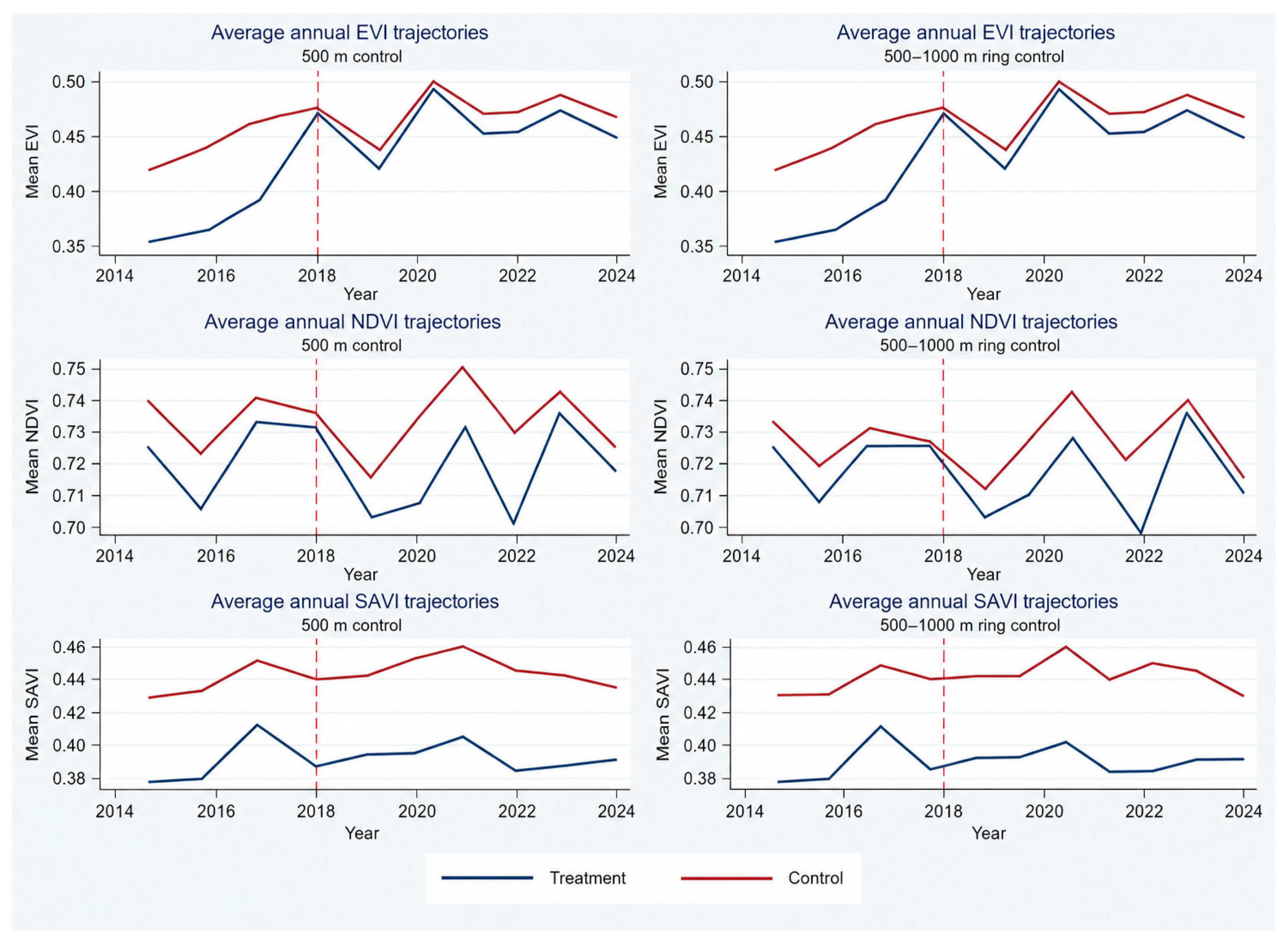
Three complementary diagnostics were implemented. First, annual average trajectories were visually compared between treated and untreated units for the 2015–2017 period. Second, a linear pre-treatment trend test was estimated using only observations from 2015 to 2017:

$$Y_{it}^k={\alpha }_{i }+{\gamma }_t+\beta \left({Treated}_i\times {Time}_t\right)+{\epsilon }_{it}$$

(6)

The time-invariant treatment main effect was omitted because it is absorbed by the spatial-unit fixed effects. ${Time}_t$ is a linear time trend centered in 2015. The coefficient ${\beta }_3$ indicates whether treated and untreated units followed different slopes before PES implementation.

Third, placebo tests were estimated by simulating false treatment start dates prior to the actual implementation period. The specifications assigned false post-treatment periods to 2017 and to 2016–2017. These placebo tests were used to identify whether apparent treatment-associated differentials existed before the program began and to assess counterfactual credibility [30,34].

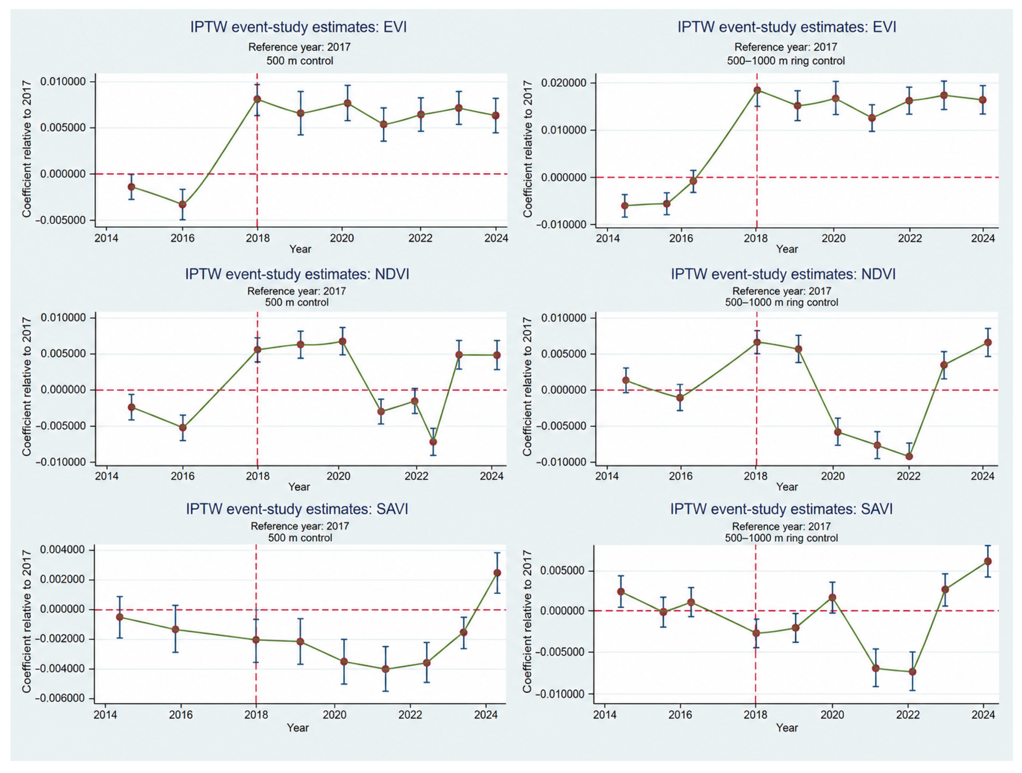
In addition, event-study specifications were estimated using 2017 as the reference year:

$$Y_{it}^k={\alpha }_{i }+{\gamma }_t+{\sum }_{t\ne 2017}{\theta }_t\left({Treated}_i \times 1\left[t=\tau \right]\right)+{\epsilon }_{it}$$

(7)

Here, $1\left[t=\tau \right]$ is an indicator for year τ, and each coefficient ${\theta }_t$ measures the treated–control differential in that year relative to 2017. The event-study models were used as diagnostic and descriptive tools to examine the temporal pattern of the estimated associations before and after the beginning of the implementation phase [30,31].

2.5. Propensity Score Estimation and IPTW Adjustment

Because enrollment in the PES program was not random, propensity-score estimation and inverse probability of treatment weighting were used to improve observable comparability between treated and untreated spatial units. The propensity score estimates the probability that a unit is treated as a function of observed pre-treatment characteristics and facilitates comparisons between treated and untreated units with similar observable initial conditions [35,36].

For each vegetation index and comparison group, the propensity score was estimated using the following logistic model:

$$\widehat{P}i=Pr\left({Treated}_i=1\right|x_i)=\mathsf{\Lambda }\left({\gamma }_0+X_i^{\prime }\gamma \right)$$

(8)

where $\widehat{P}i$ is the estimated propensity score for spatial unit i, Λ(.) denotes the logistic cumulative distribution function, and Xi is the vector of observed pre-treatment vegetation and spatial covariates.

The vegetation covariates included the mean value of the corresponding index during 2015–2017, its value in 2015, its value in 2017, and its pre-treatment standard deviation. The spatial covariates included standardized distance to the nearest populated center, standardized distance to the nearest municipal seat, municipality indicator variables, and PES modality. PES modality was incorporated as a program-design stratum associated with the reference PES area, distinguishing individual PES agreements from collective agreements.

The propensity score was estimated at the spatial-point level. Consequently, properties containing more valid pixels contributed more observations to the point-level participation model and estimand. This feature was explicitly assessed through the property-year aggregation analysis described below.

After estimating the propensity score, observations outside the region of common support were excluded. Stabilized inverse probability of treatment weights were calculated separately for treated and untreated spatial units as follows:

$${SW}_i={\displaystyle \frac{Pr\left(Treated=1\right)}{\widehat{p}i}},\mathrm{i}\mathrm{f} {Treated}_i=1$$

(9)

and

$${SW}_i={\displaystyle \frac{Pr\left(Treated=0\right)}{1-\widehat{p}i}},\mathrm{i}\mathrm{f} {Treated}_i=0$$

(10)

Here, SWi denotes the stabilized weight assigned to spatial unit i, while Pr(Treated = 1) and Pr(Treated = 0) represent the marginal proportions of treated and untreated spatial units, respectively. To reduce the influence of extreme weights, stabilized weights were trimmed at the 1st and 99th percentiles. The aggregate and phased DiD models were then re-estimated using the common-support sample and the stabilized trimmed IPTW weights.

Covariate balance before and after weighting was assessed using standardized mean differences. Absolute standardized mean differences closer to zero indicate better observable balance between treated and untreated units. An absolute SMD below 0.10 was used as a conventional reference for satisfactory observable balance [36,37].

2.6. Sensitivity and Robustness Analyses

Several sensitivity analyses were implemented to assess the robustness of the estimated associations.

First, models incorporating a differential linear time trend were estimated. These models included an interaction between treatment status and a linear time trend:

$$Y_{it}^k={\alpha }_{i }+{\gamma }_t + \delta \left({Treated}_i \times {Post}_t^{2018–2024}\right) +\theta \left({Treated}_i \times {Time}_t\right)+ {\epsilon }_{it}$$

(11)

and its phased equivalent:

$$\begin{array}{cc}{Y}_{it}^k={\alpha }_{i }+{\gamma }_t +\hfill & {\delta }_1 \left({Treated}_i \times {implementation}_t^{2018–2020}\right)\hfill \\ & +{\delta }_2 \left({Treated}_i \times post{implementation}_t^{2021–2024}\right)+\theta \left({Treated}_i\times {Time}_t\right)\hfill \\ & +{\epsilon }_{it}\hfill \end{array}$$

(12)

In these specifications, Time t denotes a linear time trend defined as year 2015 and therefore centered in 2015, and the interaction ${Treated}_i \times {Time}_t$ allows treated and untreated spatial units to follow different underlying linear temporal trajectories. The coefficient θ captures the differential linear trend between the two groups, while δ, δ1 and δ2 represent the adjusted treatment-period differentials after accounting for this additional trend. Both differential-trend specifications were estimated using the common-support sample, stabilized IPTW weights trimmed at the 1st and 99th percentiles, and spatial-unit and year fixed-effects.

These models were interpreted as stringent sensitivity analyses because they introduce additional functional-form assumptions regarding differential time dynamics between treated and untreated units. They were not adopted as the main specification, but rather as robustness contrasts, consistent with recent recommendations on pre-trend assessment and sensitivity analysis in difference-in-differences designs [34,38].

Second, the models were re-estimated after aggregating the data at the property-year–treatment-group level. This analysis reduced the dominance of properties containing large numbers of valid pixels and allowed the results to be compared with estimates obtained using a more aggregated spatial unit.

Third, a property-level parallel-trends subsample was constructed. For each property, a pre-treatment trend model was estimated using only observations from 2015 to 2017:

$$Y_{ipt}^k= {\beta }_{0p}+{\beta }_{1p}{Treated}_i + {\beta }_{2p}{Time}_i+{\beta }_{3p}\left({Treated}_i \times {Time}_t\right)+{\epsilon }_{ipt}$$

(13)

where (p) identifies the property, (i) identifies the spatial unit within the property, and (t) identifies the year. The coefficient ${\beta }_{3p}$ measures the difference in pre-treatment slope between treated and untreated units within property p.

A property was retained when it simultaneously met four predefined criteria:

• p ≥ 0.10 for the differential pre-treatment slope.
• $\left|{\beta }_{3p}\right|$ ≤ 0.02.
• Maximum absolute annual change in the treated–control pre-treatment gap ≤0.02.
• Complete treated–control gaps for 2015, 2016, and 2017.

The maximum gap change was calculated from the differences between the treated–control gaps in 2015, 2016, and 2017. Selection was based exclusively on pre-treatment information and was not conditioned on post-treatment results, thereby avoiding subsample selection based on estimated treatment-period associations [34,38]. The unweighted and IPTW-weighted DiD models were then re-estimated in this restricted sample.

Fourth, the entire empirical sequence was replicated for NDVI, EVI, and SAVI under the two control definitions.

All statistical analyses were conducted in Stata 17. Fixed-effects models included spatial-unit and year fixed-effects. Point-level models were estimated using both spatial-unit- and property-clustered standard errors. Because PES participation was assigned at the property or PES-polygon level, property-clustered inference was prioritized in the main tables, figures, and interpretation. Spatial-unit-clustered estimates were retained as supplementary sensitivity results. Property-year models were also clustered at the property level. Because treatment status is time-invariant within each spatial unit, its main effect is absorbed by the spatial-unit fixed effects. Therefore, interpretation focused on the interactions between treatment status and the temporal indicators.

3. Results

3.1. Analytical Samples and Descriptive Vegetation Trajectories

Analyses were conducted separately for NDVI, EVI, and SAVI under the 500 m neighboring control and the external 500–1000 m buffer-ring control, yielding six analytical scenarios. After quality and range cleaning, the final panels contained between 1,116,890 and 2,584,103 point-year observations. A total of 146 observations were excluded from the NDVI 500 m scenario, 1288 from the external NDVI scenario, and 47 from the external EVI scenario; no out-of-range values were identified in the remaining scenarios. Because each index used its own valid-pixel sample, cross-index comparisons represent complementary robustness assessments rather than exact replications over identical spatial observations (Figure 3).

The descriptive trajectories showed baseline treated–control differences in several scenarios. Treated NDVI values were generally slightly lower than control values before implementation, while SAVI also displayed visible baseline gaps. Some EVI trajectories separated more clearly after 2018 (

Table 1. Analytical samples by vegetation index and comparison group.

Vegetation Index	Comparison Group	Final Point-Year Observations	Property Clusters
NDVI	500 m neighboring control	1,288,804	191
NDVI	External 500–1000 m buffer-ring control	2,094,042	220
EVI	500 m neighboring control	1,604,400	214
EVI	External 500–1000 m buffer-ring control	2,584,103	239
SAVI	500 m neighboring control	1,116,890	168
SAVI	External 500–1000 m buffer-ring control	1,787,610	210

Note. Property clusters correspond to unique property identifiers in the complete valid analytical sample.

). These patterns are unadjusted and should not be interpreted as evidence of a persistent or causal program-associated vegetation response.

3.2. Counterfactual Diagnostics and Covariate Balance

Counterfactual credibility varied across vegetation indices and comparison-group definitions. With property-clustered inference, differential pre-treatment slopes were not statistically distinguishable from zero for NDVI or EVI, but remained positive and significant for SAVI under both control definitions. Placebo evidence also persisted for NDVI and SAVI in selected scenarios. These results do not imply that every specification violated parallel trends, but failure to reject a differential slope is not proof of comparability because only three pre-treatment years were available.

IPTW improved observable balance more effectively under the neighboring controls than under the external buffer-ring controls. The neighboring scenarios retained maximum post-weighting absolute standardized mean differences between 0.136 and 0.157, whereas the corresponding values for the external controls ranged from 0.283 to 0.320. Thus, weighting reducedbut did not eliminateobservable differences, particularly in the external-control specifications (

Table 2. Summary of pre-treatment diagnostics and post-IPTW covariate balance. 

Index	Pre-Treatment Trend Estimate [95% CI]	Significant Placebo Evidence	Pre-Treatment Mean SMD Before → After	Maximum Post-IPTW |SMD|	Covariates with |SMD| ≥ 0.10
NDVI—500 m neighboring	0.0038 [−0.0008, 0.0083]; p = 0.107	2017: p = 0.023	−0.128 → 0.006	0.155	5/26
NDVI—External 500–1000 m	0.0033 [−0.0019, 0.0084]; p = 0.213	None at 5%	−0.030 → −0.098	0.320	8/26
EVI—500 m neighboring	0.0019 [−0.0027, 0.0066]; p = 0.415	None at 5%	−0.613 → −0.094	0.136	4/28
EVI—External 500–1000 m	0.0036 [−0.0019, 0.0091]; p = 0.196	None at 5%	−0.622 → −0.211	0.283	12/28
SAVI—500 m neighboring	0.0051 [0.0002, 0.0099]; p = 0.041	2017: p = 0.022	−0.601 → −0.065	0.157	5/26
SAVI—External 500–1000 m	0.0058 [0.0001, 0.0115]; p = 0.046	2016–2017: p = 0.034	−0.554 → −0.172	0.302	15/26

).

Taken together, the diagnostics support interpreting the weighted coefficients as adjusted associations rather than effects obtained from fully balanced or demonstrably parallel counterfactuals. The 500 m neighboring controls generally offered better observable comparability, while the external controls reduced immediate adjacency at the cost of larger residual imbalance.

3.3. Main IPTW Difference-in-Differences Estimates

The unweighted coefficients changed substantially after common-support restriction and IPTW, particularly for EVI, indicating that observable pre-treatment differences contributed to the initial treated–control differentials.

Table 3. Main IPTW difference-in-differences estimates with property-clustered inference. 

Index	General, 2018–2024	Implementation, 2018–2020	Post-Implementation, 2021–2024	Observations	Property Clusters
NDVI—500 m neighboring	0.00364 [0.00004, 0.00723]; p = 0.048	0.0054 [0.0013, 0.0095]; p = 0.011	0.0023 [−0.0018, 0.0065]; p = 0.272	1,284,494	187
NDVI—External 500–1000 m	−0.0002 [−0.0045, 0.0040]; p = 0.909	0.0023 [−0.0029, 0.0075]; p = 0.387	−0.0021 [−0.0069, 0.0026]; p = 0.374	2,005,498	207
EVI—500 m neighboring	0.0085 [−0.0055, 0.0226]; p = 0.232	0.0092 [−0.0054, 0.0237]; p = 0.217	0.0081 [−0.0057, 0.0219]; p = 0.248	1,600,500	212
EVI—External 500–1000 m	0.0202 [0.0009, 0.0395]; p = 0.041	0.0210 [0.0009, 0.0412]; p = 0.041	0.0196 [0.0007, 0.0384]; p = 0.042	2,510,180	236
SAVI—500 m neighboring	−0.0013 [−0.0044, 0.0018]; p = 0.410	−0.0019 [−0.0058, 0.0020]; p = 0.333	−0.0008 [−0.0041, 0.0024]; p = 0.610	1,114,590	168
SAVI—External 500–1000 m	−0.0023 [−0.0061, 0.0015]; p = 0.235	−0.0002 [−0.0051, 0.0048]; p = 0.949	−0.0039 [−0.0076, −0.0001]; p = 0.043	1,736,830	200

Note. Entries report coefficients followed by property-clustered 95% confidence intervals and p-values. Models include spatial-unit and year fixed-effects, are restricted to common support, and use stabilized weights trimmed at the 1st and 99th percentiles.

therefore prioritizes the IPTW estimates with property-clustered inference.

For NDVI, the 500 m neighboring-control specification produced a small positive association for 2018–2024 and a stronger implementation-period association, while the post-implementation coefficient was not significant. None of the external-control NDVI estimates was statistically distinguishable from zero. EVI estimates were positive but imprecise under the neighboring control; the external-control estimates were positive across all phases, although this scenario retained substantial residual imbalance. SAVI provided no positive evidence, and only the negative post-implementation coefficient under the external control was statistically significant.

Relative magnitudes also differed across indices. The positive NDVI implementation coefficient under the neighboring control represented approximately 0.74% of the weighted treated-group pre-treatment mean and a standardized association of 0.046. The external-control EVI implementation estimate represented approximately 5.18% of baseline and a standardized association of 0.165, but its interpretation is limited by residual imbalance and aggregation sensitivity. The negative external-control SAVI post-implementation coefficient represented approximately −0.93% of baseline and a standardized association of −0.034.

3.4. Dynamic and Robustness Analyses

The IPTW event-study models used 2017 as the reference year and property-clustered confidence intervals. The 2015 and 2016 coefficients were not statistically significant at the 5% level in any scenario, but the short pre-treatment period and wide confidence intervals prevent interpreting this result as confirmation of parallel trends (Figure 4).

The dynamic estimates were heterogeneous. NDVI showed a positive coefficient in 2018 under the neighboring control and a negative coefficient in 2021 under the external control. EVI coefficients were positive after 2018 under both controls but were not statistically significant by individual year. SAVI showed no year-specific positive evidence (

Table 4. Phased IPTW estimates from complementary robustness analyses. 

Index	Implementation, 2018–2020	Post-Implementation, 2021–2024	Observations	Property Clusters
Panel A. Differential-Trend IPTW Models
NDVI—500 m neighboring	0.0026 [−0.0035, 0.0086]; p = 0.406	−0.0038 [−0.0133, 0.0056]; p = 0.424	1,284,494	187
NDVI—External 500–1000 m	−0.0033 [−0.0111, 0.0045]; p = 0.406	−0.0142 [−0.0268, −0.0017]; p = 0.027	2,005,498	207
EVI—500 m neighboring	0.0085 [−0.0060, 0.0230]; p = 0.248	0.0067 [−0.0072, 0.0206]; p = 0.344	1,600,500	212
EVI—External 500–1000 m	0.0184 [−0.0021, 0.0389]; p = 0.078	0.0138 [−0.0062, 0.0338]; p = 0.175	2,510,180	236
SAVI—500 m neighboring	−0.0052 [−0.0111, 0.0008]; p = 0.087	−0.0079 [−0.0173, 0.0016]; p = 0.101	1,114,590	168
SAVI—External 500–1000 m	−0.0061 [−0.0127, 0.0004]; p = 0.066	−0.0168 [−0.0274, −0.0062]; p = 0.002	1,736,830	200
Panel B. Property-Year IPTW Models
NDVI—500 m neighboring	0.0027 [−0.0045, 0.0099]; p = 0.468	0.0027 [−0.0045, 0.0100]; p = 0.457	3360	187
NDVI—External 500–1000 m	0.0004 [−0.0066, 0.0074]; p = 0.911	0.0004 [−0.0070, 0.0078]; p = 0.912	3410	206
EVI—500 m neighboring	−0.0289 [−0.0434, −0.0145]; p < 0.001	−0.0186 [−0.0320, −0.0052]; p = 0.007	3840	211
EVI—External 500–1000 m	−0.0198 [−0.0355, −0.0040]; p = 0.014	−0.0107 [−0.0258, 0.0044]; p = 0.162	3880	235
SAVI—500 m neighboring	−0.0005 [−0.0063, 0.0053]; p = 0.873	0.0033 [−0.0028, 0.0094]; p = 0.289	2950	167
SAVI—External 500–1000 m	0.0006 [−0.0061, 0.0073]; p = 0.855	0.0001 [−0.0064, 0.0065]; p = 0.988	3130	200
Panel C. Restricted Pre-Treatment-Comparable Properties
NDVI—500 m neighboring	0.0088 [0.0007, 0.0168]; p = 0.034	0.0009 [−0.0053, 0.0072]; p = 0.760	301,350	32
NDVI—External 500–1000 m	0.0010 [−0.0148, 0.0167]; p = 0.893	−0.0015 [−0.0115, 0.0085]; p = 0.748	121,103	10
EVI—500 m neighboring	0.0008 [−0.0273, 0.0289]; p = 0.956	0.0010 [−0.0238, 0.0257]; p = 0.938	361,480	43
EVI—External 500–1000 m	0.0225 [−0.0418, 0.0867]; p = 0.470	0.0276 [−0.0317, 0.0868]; p = 0.339	221,010	17
SAVI—500 m neighboring	−0.0018 [−0.0098, 0.0062]; p = 0.655	−0.0030 [−0.0072, 0.0011]; p = 0.148	241,640	31
SAVI—External 500–1000 m	0.0012 [−0.0072, 0.0096]; p = 0.764	−0.0068 [−0.0158, 0.0022]; p = 0.126	234,490	14

Note. Entries report coefficients followed by property-clustered 95% confidence intervals and p-values. Panel A includes a treatment-specific linear trend. Panel B aggregates outcomes to the property-year–treatment-group level. Panel C restricts the point-level sample to properties satisfying the predefined pre-treatment comparability criteria.

).

The robustness analyses did not identify a positive association that was invariant to analytical choices. Differential-trend adjustment removed the main NDVI implementation and EVI associations at the 5% level and produced negative post-implementation coefficients for external-control NDVI and SAVI. Property-year aggregation rendered all NDVI and SAVI estimates non-significant and reversed the EVI coefficients. In the restricted samples, the only positive coefficient that remained statistically significant was NDVI during implementation under the neighboring control; the small number of retained properties substantially reduced precision and generalizability.

3.5. Cross-Specification Synthesis

Across specifications, no vegetation index produced a uniformly positive and persistent adjusted association. For NDVI, the most recurrent positive signal was a small implementation-period association under the 500 m neighboring control. This result also appeared in 2018 and in the restricted pre-treatment-comparable sample, but it was not preserved after differential-trend adjustment or property-year aggregation.

EVI was the most sensitive index. Point-level estimates were positive under the external control, but this scenario retained substantial residual imbalance, annual coefficients were imprecise, and the property-year estimates became negative. The results therefore do not support characterizing EVI as consistently positive across counterfactual and aggregation choices.

SAVI provided no positive robustness support. Some external-control specifications showed negative post-implementation differentials, but these were not preserved after property-year aggregation or in the restricted samples and were accompanied by significant pre-treatment diagnostics. Overall, the evidence supports specification-dependent adjusted associations rather than a uniform or causally attributable improvement in vegetation condition.

4. Discussion

The results indicate that the association between participation in the Yo Protejo ¡Agua para Todos! PES program and vegetation dynamics in Cundinamarca was neither uniform across vegetation indices nor stable across comparison-group definitions, temporal phases, levels of statistical clustering, and spatial units of analysis. No vegetation index produced consistently positive and statistically robust associations across the complete set of specifications. The positive signal observed most recurrently in the point-level analyses corresponded to NDVI during the active implementation period under the 500 m neighboring-control definition. However, this association was not preserved in the differential-trend or property-year models. EVI produced positive point-level estimates under the external control but was highly sensitive to residual covariate imbalance and spatial aggregation, whereas SAVI provided no evidence of a positive adjusted association. These findings therefore support an interpretation based on specification-dependent and temporally heterogeneous associations rather than a single program response.

The NDVI results suggest a modest vegetation-greenness differential concentrated around the active implementation period. Under the neighboring-control specification, the IPTW implementation coefficient remained statistically significant after clustering standard errors at the property level; a positive annual coefficient was observed in 2018, and a positive implementation association was also identified in the restricted sample of properties satisfying the pre-treatment comparability criteria. The magnitude represented approximately 0.74% of the weighted treated-group pre-treatment mean and a standardized association of 0.046, indicating a small difference in vegetation greenness. Nevertheless, the coefficient was not statistically distinguishable from zero after introducing a differential linear trend or aggregating observations to the property-year level. Consequently, the NDVI evidence is compatible with a short-lived or localized implementation-period association, but it does not demonstrate a persistent improvement in vegetation condition attributable to PES participation.

The EVI findings require an even more cautious interpretation. In the main point-level IPTW models, the estimates obtained with the 500 m neighboring control were positive but statistically imprecise after clustering at the property level. Positive and statistically significant coefficients were obtained under the external 500–1000 m buffer-ring control, with the implementation estimate representing approximately 5.18% of the weighted baseline mean and a standardized association of 0.165. However, this scenario retained substantial residual imbalance in pre-treatment vegetation, settlement-distance, PES-modality, and municipality covariates. Moreover, the annual event-study coefficients were not statistically significant at the 5% level, the differential-trend estimates weakened, the restricted property-level estimates were imprecise, and the property-year IPTW coefficients changed sign and became negative. The EVI results therefore cannot be characterized as the most consistent positive evidence. Instead, they demonstrate pronounced sensitivity to counterfactual construction, weighting, and the relative contribution of properties containing different numbers of valid pixels.

SAVI did not provide positive robustness support. The neighboring-control estimates were generally close to zero and statistically non-significant after property-level clustering. Under the external comparison, the main IPTW and differential-trend models identified negative post-implementation associations. The main post-implementation coefficient represented approximately −0.93% of the treated-group baseline mean and a standardized association of −0.034. However, SAVI also retained statistically significant differential pre-treatment slopes under both control definitions, and the negative post-implementation coefficient was not preserved in the property-year or restricted parallel-trends analyses. Accordingly, this result should not be interpreted as evidence that PES participation reduced vegetation condition. It is more appropriately understood as a partial negative differential arising in a comparison-group specification with remaining identification limitations.

The divergence among NDVI, EVI, and SAVI may reflect both ecological and measurement-related mechanisms. NDVI is widely used to represent vegetation greenness and photosynthetic activity but can become less sensitive under relatively dense canopy conditions and may be influenced by atmospheric and background characteristics [17,26]. EVI incorporates the blue band and additional gain and correction parameters to reduce some atmospheric and canopy-background influences and to retain sensitivity under higher biomass conditions [18]. SAVI, in contrast, explicitly reduces the influence of soil background and may respond differently in heterogeneous rural mosaics containing pastures, crops, secondary vegetation, sparse cover, and exposed soil [19]. These properties provide plausible reasons why the indices may not respond identically to changes in vegetation condition.

Nevertheless, the differences among indices should not be interpreted as purely ecological mechanisms. Each index was estimated using its own set of valid pixels after quality filtering, and the property-year analyses altered the relative contribution of properties with different numbers of spatial observations. The reversal of the EVI coefficients after aggregation is particularly important because it indicates that the positive point-level pattern may have been influenced by the spatial distribution and weighting of valid pixels rather than by a uniform ecological response across properties. The observed index heterogeneity therefore likely combines differences in spectral sensitivity, land-cover composition, valid-pixel samples, spatial aggregation, and residual confounding. Future evaluations should examine these mechanisms directly by stratifying results according to baseline land cover, canopy density, soil exposure, elevation, ecosystem type, and productive land use.

The credibility of the estimated associations also depends fundamentally on the construction of the counterfactual and the treatment of endogeneity. PES enrollment was not randomly assigned, and participating properties may differ systematically from untreated areas in ecosystem importance, previous degradation, management history, accessibility, institutional attention, and expected conservation potential [9,10,11,21,22]. Spatial-unit and year fixed effects control for time-invariant differences across observation points and common annual shocks, while IPTW reduces imbalance in observed pre-treatment vegetation and spatial characteristics [35,36,37]. However, neither strategy eliminates bias from unobserved or time-varying factors.

The updated pre-treatment diagnostics illustrate this limitation. When standard errors were clustered at the property level, differential pre-treatment slopes were not statistically significant for NDVI or EVI, but remained significant for SAVI. Some placebo coefficients also remained significant, particularly the 2017 placebo for NDVI and SAVI under the neighboring-control definition and the 2016–2017 placebo for SAVI under the external control. Failure to reject a pre-treatment coefficient equal to zero does not demonstrate that the parallel-trends assumption was satisfied, especially with only three pre-treatment years and relatively wide property-clustered confidence intervals [30,34,38]. These mixed diagnostics justify interpreting the DiD coefficients as adjusted associations rather than as causally identified treatment effects.

The level of statistical clustering was itself substantively important. The original point-level panel contained very large numbers of spatial observations, but pixels located within the same property are exposed to common management practices, environmental conditions, program assignment, and local shocks. Clustering standard errors at the property level substantially widened confidence intervals and rendered several coefficients that were statistically significant under spatial-unit clustering indistinguishable from zero. This finding demonstrates that the large number of pixels should not be interpreted as an equally large number of independent treatment assignments. Aligning statistical inference with the property level therefore provides a more conservative and credible assessment of uncertainty.

The comparison-group results also reveal a trade-off between spatial proximity and statistical independence. The neighboring 500 m controls achieved substantially better observable balance after IPTW and are more likely to share local environmental conditions with treated areas. However, they may also be affected by spillovers, shared land-management practices, hydrological connectivity, or indirect institutional influence. The external 500–1000 m buffer-ring reduces immediate adjacency and potential contamination, but it exhibited substantially greater residual imbalance in vegetation, distance, PES modality, and municipality indicators. The positive external-control EVI estimates and the negative external-control SAVI and NDVI differentials must therefore be interpreted in light of weaker observable comparability. More distant controls did not automatically provide a more credible counterfactual.

Temporal heterogeneity remains an important feature of the evidence, although it should not be generalized across all indices. The most recurrent positive NDVI signal was concentrated during 2018–2020 and was not maintained consistently during 2021–2024. This pattern could be compatible with stronger compliance, monitoring, technical assistance, or behavioral responses while the program was actively implemented. Previous research has shown that conservation-incentive outcomes may depend on targeting, conditionality, incentive continuity, monitoring, and contract duration [2,4,8,12,13,14,39,40,41]. However, the available data do not permit direct testing of these mechanisms. The implementation-period pattern should therefore be presented as a plausible temporal interpretation rather than as evidence that program activities generated the observed changes.

The robustness analyses further limit any simple success-or-failure interpretation. Differential-trend models weakened most positive point-level associations. Property-year aggregation eliminated the positive NDVI signal and reversed the EVI estimates. The restricted parallel-trends samples retained only a positive NDVI implementation coefficient under the neighboring control, while EVI and SAVI estimates remained statistically imprecise. In addition, only a small proportion of properties satisfied the predefined pre-treatment comparability criteria, particularly under the external-control definitions. These restricted analyses improve internal comparability but substantially reduce statistical precision and external generalizability. Taken together, the robustness evidence indicates that no estimated association is invariant to the analytical choices considered.

From a policy perspective, the findings demonstrate that PES performance cannot be inferred solely from enrolled area, number of participants, executed resources, or a single satellite vegetation indicator. Administrative indicators remain essential for monitoring program delivery, but they do not establish measurable environmental outcomes. Monitoring systems should combine multiple longitudinal ecological indicators with information on contract duration, payment continuity, compliance, technical assistance, monitoring frequency, land-use practices, and baseline ecosystem conditions. They should also recognize the hierarchical structure of spatial data and report inference at the level at which program participation is assigned.

The study therefore contributes less by providing a definitive judgment regarding the environmental effectiveness of the evaluated PES program than by demonstrating how strongly that judgment depends on the vegetation metric, comparison-group construction, weighting strategy, inferential level, temporal specification, and spatial aggregation. The integrated use of multiple indices, alternative counterfactuals, property-clustered inference, balance diagnostics, event-study models, differential trends, and property-level robustness analyses provides a more transparent framework for evaluating conservation incentives. For Cundinamarca, the evidence supports only a modest and specification-sensitive NDVI association during active implementation, rather than a uniform, persistent, or causally attributable improvement in vegetation condition.

5. Conclusions

This study evaluated the association between participation in the Yo Protejo ¡Agua para Todos! Payments for Ecosystem Services program and satellite-based vegetation dynamics in Cundinamarca, Colombia, during the period of 2015–2024. The analysis combined Landsat-derived NDVI, EVI, and SAVI observations with fixed-effects difference-in-differences models, propensity-score weighting, alternative spatial comparison groups, property-clustered inference, event-study diagnostics, and complementary robustness analyses.

The results do not support a uniform or persistent positive association between PES participation and vegetation condition. The most recurrent positive signal was a small NDVI association during the 2018–2020 implementation period under the 500 m neighboring-control definition. This association was also observed in 2018 and in the restricted pre-treatment-comparable sample, but it was not preserved after differential-trend adjustment or property-year aggregation. EVI produced positive point-level estimates under the external control, although this specification retained substantial residual covariate imbalance and the estimates became negative after property-year aggregation. SAVI provided no robust positive evidence, while the negative post-implementation differentials identified in some external-control models were not stable across robustness specifications.

These findings demonstrate that the estimated associations were sensitive to the vegetation index, comparison-group definition, temporal phase, inferential level, and spatial unit of analysis. IPTW improved observable comparability but did not eliminate residual imbalance, and property-level clustering substantially widened confidence intervals relative to spatial-unit clustering. Accordingly, the results should be interpreted as specification-dependent adjusted associations rather than definitive causal effects. The evidence does not establish that the program uniformly improved or deteriorated vegetation condition, nor that favorable differentials persisted after implementation ended.

Beyond the evidence for Cundinamarca, the study contributes an integrated framework for evaluating conservation-incentive programs through longitudinal remote sensing, multiple spectral indicators, alternative spatial counterfactuals, numerical balance diagnostics, property-level inference, and complementary sensitivity analyses. This approach provides a more transparent basis for assessing environmental performance than administrative indicators or simple before-and-after comparisons alone.

6. Limitations and Future Research

This study has several limitations that should be considered when interpreting its findings. First, NDVI, EVI, and SAVI are indirect indicators of vegetation greenness and spectral condition. They do not directly measure forest cover, biodiversity, biomass, habitat quality, ecological integrity, water regulation, or ecosystem-service provision. Future studies should therefore combine vegetation indices with land-cover classifications, forest-structure metrics, hydrological indicators, biodiversity data, and field observations.

Second, each vegetation index was analyzed using its own valid-pixel sample after quality filtering and range cleaning. Consequently, differences among NDVI, EVI, and SAVI may reflect both their distinct spectral properties and variation in the spatial composition of the analytical samples. Harmonized pixel samples, multi-index models, and analyses stratified by land cover, canopy density, and soil exposure would help clarify the mechanisms underlying index heterogeneity.

Third, PES participation was not randomly assigned. Fixed-effects and IPTW improved observable comparability but could not eliminate bias from unobserved or time-varying factors such as previous land-use trajectories, livestock intensity, management practices, technical assistance, compliance, institutional capacity, local enforcement, and microclimatic conditions. In addition, the three-year pre-treatment period limited the statistical power of parallel-trends and placebo diagnostics. Future evaluations would benefit from longer pre-intervention series, richer administrative and environmental covariates, and designs exploiting exogenous variation in eligibility, timing, or program assignment.

Fourth, the hierarchical and spatial structure of the data affected statistical inference. Although the panel contained large numbers of pixels, observations within the same property shared treatment assignment and local environmental conditions. Property-level clustering therefore produced wider and more credible confidence intervals than spatial-unit clustering. Results were also sensitive to property-year aggregation, especially for EVI, indicating that the relative influence of properties with different numbers of valid pixels matters. Future studies should consider multilevel models, property-weighted estimators, and alternative aggregation strategies.

Fifth, neither spatial comparison group provided a fully satisfactory counterfactual. The 500 m neighboring controls achieved better observable balance but may have been affected by spillovers, shared management, or spatial dependence. The external 500–1000 m buffer-ring reduced immediate adjacency but retained greater covariate imbalance. Future research should evaluate environmentally matched controls, watershed-based neighborhoods, alternative buffer distances, and explicit spatial-dependence models.

Finally, the available information did not permit direct analysis of implementation intensity, contract duration, payment continuity, monitoring frequency, technical assistance, or compliance with conservation agreements. The 2015–2024 period may also be insufficient to detect delayed ecological responses or long-term behavioral changes. Linking remote sensing outcomes with detailed administrative records, extending the monitoring horizon, and incorporating higher-resolution imagery and field data would improve understanding of when and under what conditions PES programs are associated with sustained environmental outcomes.