Article

Ecological Network Bottlenecks and Restoration Priorities in the Chengjiang Karst Basin, China

1
Institute of Architecture and Urban Planning, Chongqing University, Chongqing 400045, China
2
Institute of Resources and Environment, Lanzhou University, Lanzhou 730000, China
*
Author to whom correspondence should be addressed.
Land 2026, 15(8), 1332; https://doi.org/10.3390/land15081332
Submission received: 3 June 2026 / Revised: 15 July 2026 / Accepted: 16 July 2026 / Published: 24 July 2026
(This article belongs to the Special Issue Spatial Optimization for Multifunctional Land Systems)

Abstract

Karst river basins require restoration approaches that identify vulnerable connections while distinguishing ecological constraints from governance implementation conditions. This study developed a sequential Structure–Resistance–Connectivity–Governance (SRCG) framework for the Chengjiang River Basin, Guangxi, China. Ecological sources were identified from vegetation vitality, habitat quality, landscape integrity, and hydrological proximity. Natural landscape resistance and anthropogenic disturbance were integrated to delineate potential source-pair corridors. Bottleneck Intensity combined corridor load, minimum corridor width, and high-resistance overlap, and was integrated with ecological movement resistance to delineate Ecological Restoration Priority Zones (ERPZs). Governance Mismatch Index and Administrative Boundary Proximity Index values were applied only after ERPZ delineation. The analysis identified 28 ecological sources covering 312.4 km2, 76 potential connections, three principal bottleneck clusters, and six ERPZs covering 118.5 km2. The upper basin retained a relatively continuous network; whereas, the middle and lower reaches were increasingly constrained by roads, settlements, quarry disturbance, fragmented cropland, and discontinuous riparian vegetation. ERPZ-A, D, E, and F were resistance-dominated, ERPZ-B was bottleneck-dominated, and ERPZ-C was compound-priority. Governance assessment differentiated four implementation contexts. Overall land-cover accuracy was 0.896, Cohen’s kappa was 0.874, and 14 of 16 field sections were concordant with mapped landscape conditions; sensitivity tests retained the principal sources, bottlenecks, and ERPZ cores. The framework separates ecological restoration urgency from implementation difficulty, while its outputs represent potential structural rather than confirmed functional connectivity.

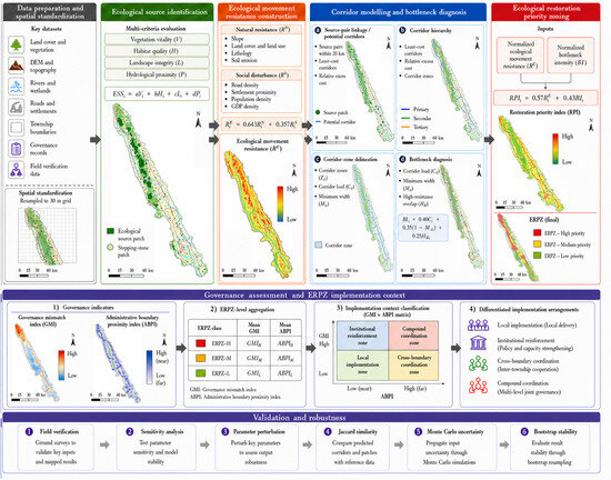
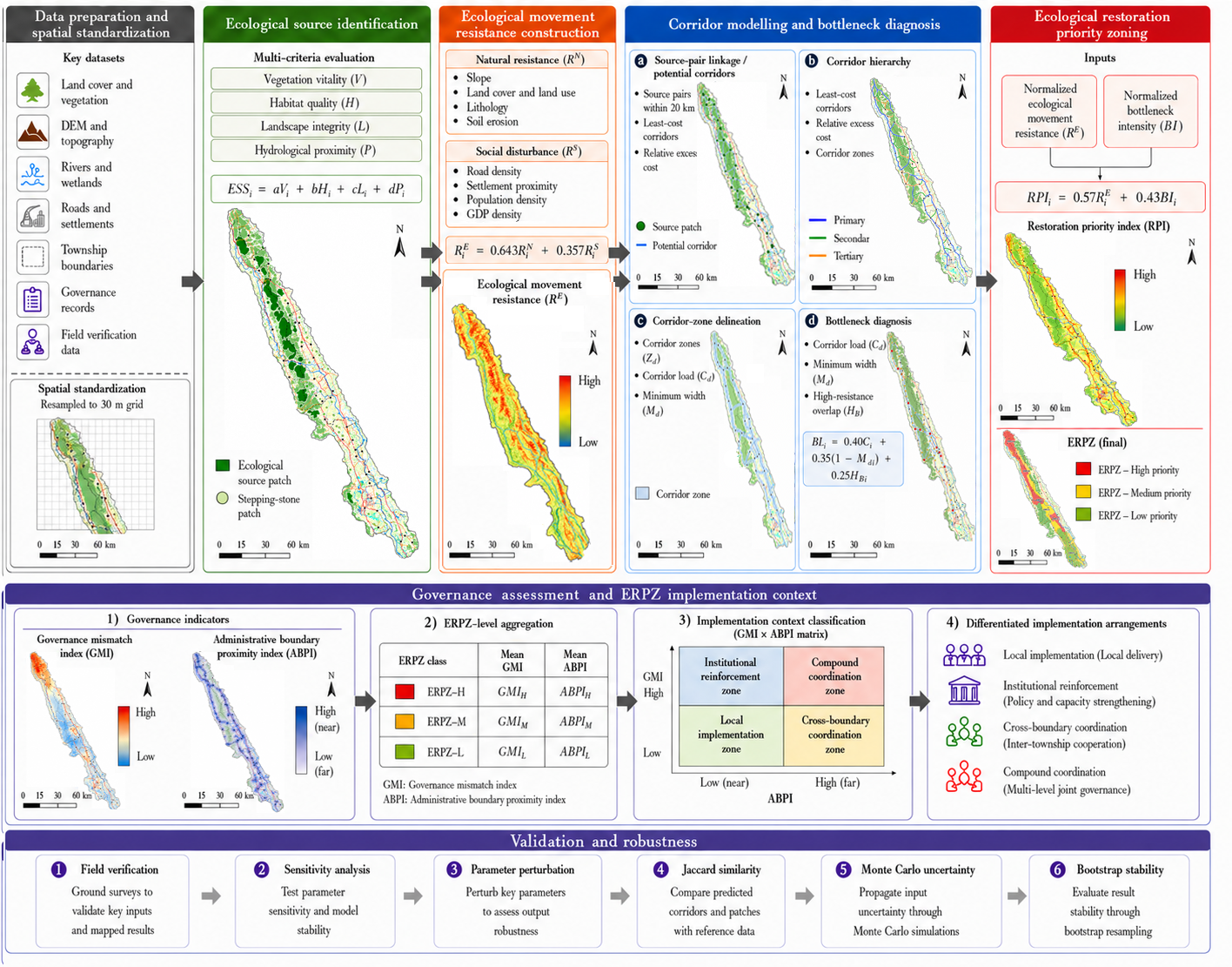
Graphical Abstract

1. Introduction

Karst river basins are ecologically fragile land systems characterised by heterogeneous terrain, shallow and discontinuous soils, exposed carbonate surfaces, complex surface–subsurface hydrological pathways, and high sensitivity to vegetation degradation and rocky desertification [1,2]. Although ecological engineering has improved vegetation growth and carbon storage in many karst areas of Southwest China [3], regional vegetation recovery does not necessarily ensure habitat continuity or landscape permeability at the basin scale. Agricultural intensification, infrastructure construction, settlement expansion, and quarry disturbance may fragment ecological land and concentrate potential connections within restricted valley floors, riparian zones, and slope–valley transitions. Graph-based indices, including the Integral Index of Connectivity and Probability of Connectivity, quantify overall network configuration and the contribution of individual habitat patches [4,5]; whereas, circuit theory and resistance-based modelling identify spatially plausible connections across heterogeneous landscapes [6,7]. However, mapping ecological sources and potential corridors alone does not reveal whether these connections remain structurally secure where multiple routes converge within narrow and highly resistant passages.
Recent ecological-network studies have extended analysis from static source–corridor identification towards dynamic assessment, multifunctional source selection, bottleneck diagnosis, and differentiated restoration zoning. Research has examined ecological-network changes under land-use/land-cover transformation [8], translated sources, corridors, pinch points, and barrier areas into restoration zones [9], and constructed ecological security patterns in the neighbouring karst region of Hechi, Guangxi [10]. Other approaches have integrated ecosystem-service supply, demand, and sensitivity [11], or combined circuit theory with dynamic weighted networks to identify conservation and restoration priorities [12]. Recent reviews consequently identify dynamic analysis, multifunctional integration, cross-scale assessment, and empirical validation as key directions for ecological-network research [13]. Policy information has also been spatially quantified within ecological-security-pattern construction [14]. More recent studies have assessed multi-temporal restoration priorities [15], combined carbon-sink performance with ecological connectivity [16], examined the long-term evolution of ecological networks [17], integrated functional and structural models in restoration zoning [18], and linked ecological security patterns with landscape ecological risk [19]. Nevertheless, two issues remain insufficiently resolved in karst-basin restoration planning. First, potential connections may remain topologically present while becoming structurally vulnerable because of corridor convergence, local constriction, and high-resistance overlap. Second, governance indicators describe the institutional conditions under which restoration is planned, financed, monitored, and maintained; they do not constitute physical or behavioural resistance to ecological movement. This distinction is important because ecological processes and administrative responsibilities frequently operate at different spatial scales [20]. These challenges may become more dynamic under climate and land-use change [21], which can exert distinct and interactive effects on ecological-network structure and connectivity.
To address these ecological and institutional challenges, this study develops a sequential Structure–Resistance–Connectivity–Governance (SRCG) framework for the Chengjiang River Basin in Guangxi, China, and addresses three questions: (1) How do ecological sources, natural resistance, and social disturbance shape potential structural connectivity in a karst basin? (2) Where do corridor convergence, spatial constriction, and high-resistance overlap generate structural bottlenecks and ecological restoration priorities? (3) How do governance mismatch and administrative boundary proximity differentiate implementation conditions after ecological priorities have been independently identified? The study first identifies ecological sources and constructs an ecological movement resistance surface, then delineates potential corridors and bottlenecks, integrates ecological movement resistance and Bottleneck Intensity to identify Ecological Restoration Priority Zones (ERPZs), and finally evaluates ERPZ-level governance implementation contexts. Its principal contribution lies in separating ecological restoration urgency from governance implementation difficulty and subsequently integrating both dimensions within basin-scale restoration planning.

2. Materials and Methods

2.1. Study Area

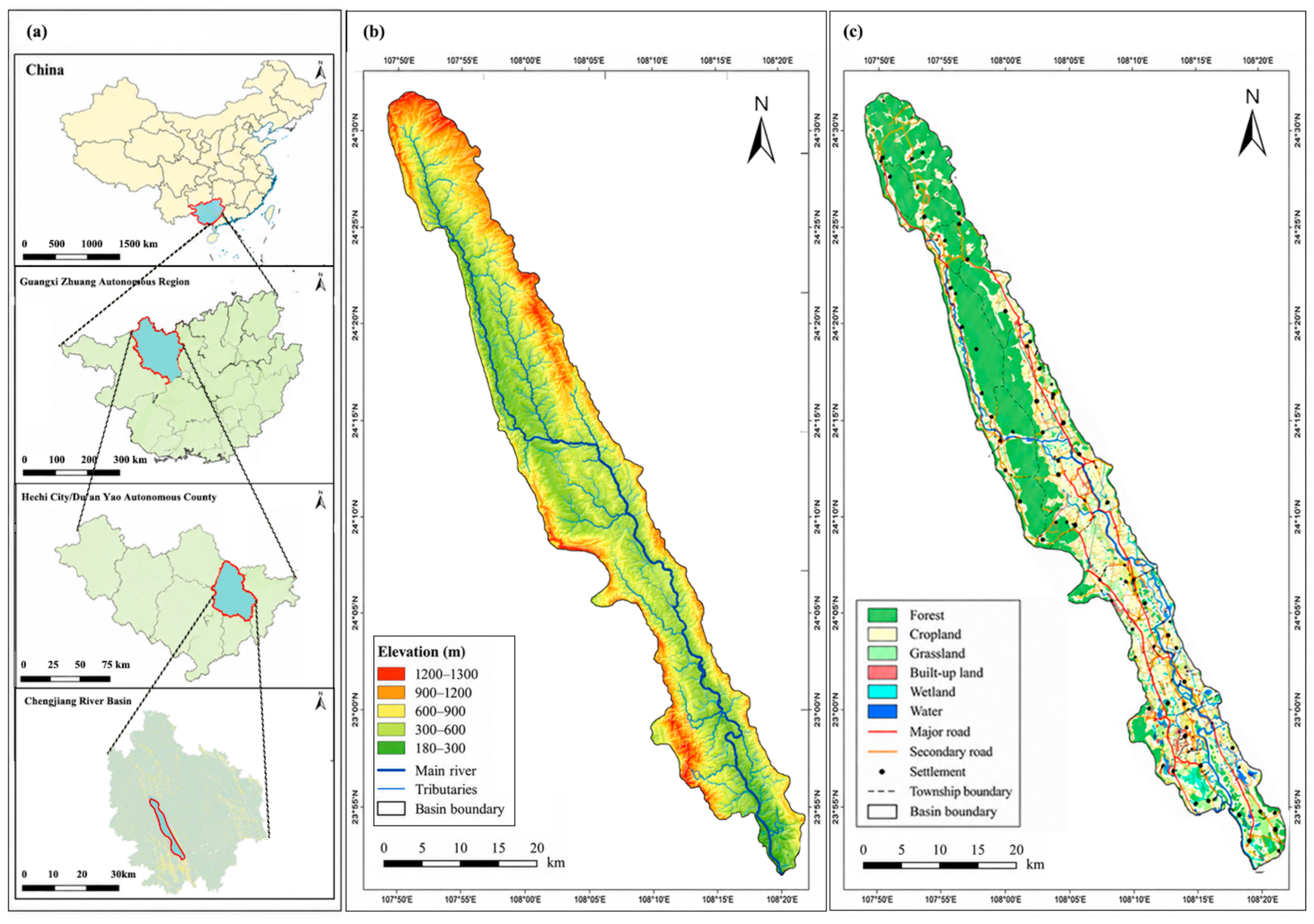
The Chengjiang River Basin (CRB) is located in northwestern Du’an Yao Autonomous County, Guangxi Zhuang Autonomous Region, southern China, between approximately 24°00′–24°32′ N and 107°50′–108°20′ E (Figure 1). The basin covers approximately 1280 km2 and forms part of the upper Hongshui River system. It is a representative karst watershed in Southwest China, where prolonged carbonate dissolution has produced tower-karst hills, enclosed depressions, sinkholes, incised valleys, and partially developed subsurface drainage. These landforms are associated with shallow and discontinuous soils, exposed bedrock, fragmented surface runoff, high erosion sensitivity, and susceptibility to rocky desertification [1,2]. The basin exhibits a pronounced upstream–downstream landscape gradient. Forest, shrubland, and relatively continuous woodland are concentrated in the upper catchments and on steeper karst slopes, where vegetation cover and habitat continuity are comparatively high. Cropland, rural settlements, roads, construction land, and localised quarry disturbance are concentrated mainly within the middle and lower valleys. The Chengjiang River, its tributaries, wetland margins, and riparian vegetation form the principal longitudinal ecological axis, while slope–valley transitions provide lateral connections between upland habitats and the valley floor.
For spatial comparison, the CRB was divided into upper, middle, and lower sections according to main-stem position and associated subcatchment structure; these divisions were used only to compare landscape and network patterns and did not influence source selection, resistance assignment, corridor delineation, or restoration-priority classification. The basin was selected because it combines representative Southwest China karst landforms with rocky-desertification and riparian-fragmentation pressures, valley-floor agriculture, settlement and transport development, and township-level coordination requirements.
Ecological processes extend across the watershed and river network; whereas, land-use regulation, fiscal support, project implementation, and maintenance are organised mainly through township administrations. Although the basin is not designated as a single national or international protected area, parts of it are subject to ecological-redline, water-resource, wetland, rocky-desertification-control, and land-use management requirements. This combination of ecological fragility, heterogeneous land use, restricted valley passages, and mismatched ecological and administrative units makes the CRB suitable for testing a framework that separates structural-connectivity diagnosis and restoration-priority identification from implementation-context assessment.

2.2. Data Sources and Preprocessing

This study integrated remote-sensing imagery, vegetation indices, terrain, lithology, soil erosion, hydrology, infrastructure, socioeconomic statistics, governance records, administrative boundaries, and field survey. These datasets supported ecological source identification, ecological movement-resistance construction, corridor and bottleneck modelling, Ecological Restoration Priority Zone (ERPZ) delineation, and post-delineation governance assessment. Table 1 summarises the principal variables, data sources, periods, native spatial scales, and analytical applications.
All spatial datasets were projected to WGS 1984 UTM Zone 48N. A 30 m grid was adopted as the common unit for spatial registration, ecological source identification, resistance modelling, corridor analysis, and restoration-priority calculation. The common grid ensured geometric consistency but did not increase the native information content of coarser datasets [22]. MODIS vegetation indices and township-level socioeconomic statistics were therefore interpreted as broad spatial gradients rather than independent observations at the 30 m scale. Governance indicators retained their original township-level meaning. Field surveys conducted from May to August 2024 recorded land-cover type, vegetation continuity, riparian condition, road and settlement disturbance, corridor constriction, exposed karst surfaces, slope degradation, and quarry disturbance.
The 2023 land-use and land-cover map was produced from Landsat 8 and Sentinel-2 L2A imagery. Sentinel-2 imagery was processed using Sen2Cor, and SCS+C correction was applied to reduce illumination differences associated with steep karst terrain [23,24]. Land-cover classification was conducted using a Random Forest classifier [25,26]. The classification comprised seven categories: forest and mixed woodland, cropland, grassland and shrubland, built-up land and settlements, bare rock and sparsely vegetated land, wetland, and water. A total of 1200 samples were used for classifier training, and 230 spatially independent samples were retained for accuracy assessment using a complete confusion matrix and class-specific accuracy measures [27,28]. Vegetation vitality was represented by the long-term MODIS NDVI and EVI series rather than by a single-date vegetation index. The time series were smoothed using a Savitzky–Golay filter and aggregated to annual values to reduce seasonal and atmospheric variation [29,30,31]. The MODIS products represented persistent vegetation condition; whereas, the 2023 Sentinel-2 classification provided the finer spatial configuration of current land cover. Although the ecological-network analysis used the 2023 land-cover map, annual classifications for 2018–2022 were also produced using the same Random Forest workflow and classification scheme. These earlier classifications were retained only to examine the temporal consistency of the classification procedure.
Elevation and derived terrain variables were calculated primarily from SRTM v3 data [32]. ASTER GDEM was used only to check the consistency of terrain patterns in areas of complex karst relief and was not combined with SRTM to create an averaged elevation surface. Lithology and soil-erosion data were used to represent carbonate-rock conditions and erosion-related landscape constraints. River networks, perennial water bodies, wetlands, and riparian zones were compiled from local records and refined through remote-sensing interpretation. Together, these datasets supported ecological source screening, habitat-quality assessment, hydrological proximity analysis, and natural resistance construction.
Anthropogenic disturbance was represented at two spatial scales. Road density and settlement proximity captured localised and spatially explicit disturbance; whereas, township-level population and GDP represented broader differences in human concentration, economic activity, and development pressure. Township values were registered to the common analytical grid but remained spatially homogeneous within each township; this procedure enabled spatial overlay and did not constitute statistical downscaling or imply independent 30 m socioeconomic observations. Population and GDP were therefore interpreted as broad background components rather than fine-scale determinants of local corridor geometry. Governance data were compiled from ecological-restoration policies, land-management documents, fiscal and ecological-compensation records, joint-monitoring records, and inter-township cooperation documents. The records covered the townships intersecting the basin and were screened using consistent inclusion criteria. Policy and management documents were coded to derive indicators of policy coordination, fiscal alignment, and cooperation frequency [33]. Coding consistency was evaluated through independent coding and intercoder agreement [34]. These indicators were retained at the township scale and were used only to characterise the implementation conditions of independently delineated ERPZs. Township boundaries were processed separately to calculate administrative boundary proximity and were not treated as ecological barriers or movement resistance.

2.3. Structure–Resistance–Connectivity–Governance Framework

The SRCG framework comprised four sequential stages: ecological source identification, ecological movement-resistance construction, corridor and bottleneck modelling, and ERPZ delineation followed by governance implementation assessment. Sources, resistance, corridors, bottlenecks, and ERPZs were derived independently of governance indicators; GMI and ABPI were applied only after ERPZ delineation. This sequence follows ecological-network and restoration-zoning logic [9,12,15,18,19] while avoiding the conversion of policy or administrative conditions into ecological movement resistance.

2.3.1. Ecological Source Identification

Ecological sources were identified by integrating vegetation vitality, habitat quality, landscape integrity, and hydrological proximity. Vegetation vitality was derived from long-term NDVI and EVI data. Habitat quality was estimated using the InVEST Habitat Quality model with roads, settlements, cropland, construction land, and quarry-affected areas as disturbance layers [35]. Landscape integrity incorporated patch area, core-area characteristics, and shape compactness [36], while hydrological proximity represented distance to perennial rivers, wetlands, and principal riparian habitats [37]. Ecological source suitability was calculated as:
ESS i = aV i + bH i + cL i + dP i
where ESS i is the ecological-source suitability of grid cell i, V i ,   H i ,   L i ,   and   P i are the normalised vegetation-vitality, habitat-quality, landscape-integrity, and hydrological-proximity indicators, respectively; and hydrological proximity indicators weights were a   =   0.25 ,   b   =   0.35 ,   c   =   0.25 ,   and   d   =   0.15 . High-suitability cells were aggregated into candidate patches. Core sources were required to have a mean NDVI of at least 0.60, a Core Area Index above 0.60, a Landscape Shape Index below 2.50, and an area of at least 1.5 km2. Smaller patches were retained only where they functioned as potential stepping stones. High-resolution imagery and field records were used to remove artefacts and recently disturbed patches. Alternative minimum source areas of 1.2 and 1.8 km2 were examined in the sensitivity analysis. This procedure retained both large habitat cores and strategically positioned connector patches.

2.3.2. Ecological Movement Resistance

Ecological movement resistance integrated natural landscape resistance and social disturbance. Governance variables and administrative boundaries were excluded because they represented implementation conditions rather than movement constraints. Natural resistance was calculated as:
R i N = k = 1 m ω k N ik
where R i N is the natural resistance of grid cell i, N ik is the normalised value of factor k and ω k is its weight. Slope, land use and land cover, vegetation condition, lithology, and erosion risk were assigned weights of 0.32, 0.28, 0.20, 0.12, and 0.08. Social disturbance was calculated as:
R i S = k = 1 n ν k S ik
where R i S is the social-disturbance value, S ik is the normalised social factor k, and ν k is its weight. Road density and settlement proximity represented localised disturbance; whereas, township-level population and GDP represented broader socioeconomic-pressure gradients. Population and GDP were not interpreted as independent 30 m observations and did not determine local corridor geometry. The integrated resistance surface was calculated as:
R i E   =   α N R i N + α S R i S , α N + α S = 1
where R i E is ecological movement resistance. The baseline weights were α N = 0.643 and α S = 0.357. For the ecological movement-resistance surface, the natural and social components were retained; whereas, governance-related conditions were assessed subsequently at the ERPZ level. The resulting R i E surface was used as the cost surface for corridor modelling.

2.3.3. Potential Corridor Modelling and Bottleneck Diagnosis

Ecological sources were treated as network nodes. Source pairs separated by no more than 20 km were retained in the baseline network, with 16 and 24 km tested as alternatives. These thresholds were treated as structural-network assumptions rather than species-specific dispersal limits [6,7,38,39,40,41]. Potential connections were identified using the Minimum Cumulative Resistance model:
MCR ab = min ρ p ab r ρ ( D r   ×   R r E )
where MCR ab is the Minimum Cumulative Resistance between sources a and b P ab is the set of candidate paths between the two sources, D r is the traversal distance through cell r and R r E is its ecological movement resistance. Standardised MCR values were classified into primary, secondary, and tertiary corridors using Jenks natural breaks. These classes represented relative conditions within the CRB rather than universal ecological thresholds. Corridor zones were delineated using relative excess cost:
R E C ab , i   =   CD a , i + CD b , i MCR ab MCR ab
where CD a , i and CD b , i are the accumulated cost distances from sources a and b to grid cell i. Cells satisfying R E C ab , i     τ were retained as corridor zone Z a b . The baseline tolerance was τ   =   0.05 , with 0.04 and 0.06 tested as alternatives. Corridor load was calculated as:
CL i = ( a , b ) Ω I ( i Z a b )
where CL i is the number of modelled source-pair corridor zones intersecting cell i, Ω is the set of retained source pairs, and I   ( ) is an indicator function. Corridor load represented modelled route convergence rather than animal abundance or movement frequency. Corridor zones were divided into successive units along their centrelines. Perpendicular cross-sections were generated at 30 m intervals, and the minimum corridor-zone width within each unit was retained. High-resistance overlap was defined as the proportion of each unit occupied by cells within the upper 20% of the basin-wide resistance distribution; upper 15% and upper 25% thresholds were also tested. After normalisation, Bottleneck Intensity (BI) was calculated as:
BI s   =   0.40 CL S   +   0.35 ( 1     MW S )   +   0.25 HR S
where CL S is normalised corridor load, MW S is normalised minimum width, and HR S is normalised high-resistance overlap. Higher values identified locations where multiple modelled connections converged within narrow and comparatively resistant landscape passages. The influence of the three component weights was evaluated by ±10% and ±20% perturbations. Candidate bottlenecks were identified from the highest BI class produced by Jenks natural breaks. Spatially contiguous high-BI units were grouped and checked against high-resolution imagery and field observations. Comparable restoration studies have identified pinch points, barrier areas, and dynamically important network locations [9,12,15,17,18,19]. Network connectivity was evaluated in Conefor [42] using source-patch area as the node attribute. Under the baseline binary rule, source pairs within 20 km were treated as connected. IIC and PC described potential structural connectivity rather than observed species movement or gene flow.

2.3.4. Ecological Restoration Priority Zoning and Governance Implementation Assessment

ERPZs were constructed by integrating normalised ecological movement resistance and BI. Ecological movement resistance represented broad reductions in landscape permeability; whereas, BI represented localised structural vulnerability. This step translated ecological-network diagnosis into mechanism-based restoration zoning before any governance indicator was applied. The Restoration Priority Index was calculated as:
RPI i   =   γ R R i E   +   γ B BI i
where RPI i is the restoration-priority value of cell i, R i E is normalised ecological movement resistance, and BI i is normalised Bottleneck Intensity. The baseline weights were γ R = 0.57   and   γ B = 0.43 . Alternative ratios of 0.50:0.50, 0.60:0.40, and 0.70:0.30 were tested. The continuous RPI surface was classified into low-, moderate-, and high-priority levels using Jenks natural breaks. Contiguous high-priority cells were aggregated into ERPZs where they coincided with source margins, corridor zones, high-BI sections, or identifiable landscape constraints. Governance indicators were not used in RPI calculation or ERPZ boundary delineation.
GMI j = 1 C j   + F j   + P j 3
where GMI j is the governance mismatch of township j, and P j , F j , and C j represent normalised policy coordination, fiscal alignment, and cooperation frequency. The equal-weight arithmetic mean was retained as a transparent baseline rather than as a universal governance model. Because it permits compensation among components, geometric aggregation and component-dominant weighting scenarios were also evaluated. Higher values indicated greater relative mismatch. Administrative-boundary exposure was calculated as:
ABPI i = e x p ( d i λ )
where d i is the distance from cell i to the nearest township boundary and λ is the decay parameter. The baseline value was 500 m, with 400 and 600 m tested as alternatives. ABPI represented proximity to an administrative interface and did not treat boundaries as ecological barriers [20,43,44,45,46]. For ERPZs spanning multiple townships, GMI was calculated as an area-weighted mean; ERPZ-level ABPI was the mean cell value. Median GMI and ABPI values were used to distinguish local implementation, institutional reinforcement, cross-boundary coordination, and compound coordination. Neither index affected resistance, corridor configuration, BI, RPI, ecological-priority type, or ERPZ boundaries.
GMI summarised township-level policy coordination, fiscal alignment, and cooperation frequency, while ABPI identified ERPZ cells located close to administrative boundaries. Both were calculated only after ecological sources, corridors, bottlenecks, and ERPZs had been delineated. Table 2 summarises the indicator definitions and normalisation rules; alternative GMI weights and ABPI decay distances were tested in the sensitivity analysis.

2.4. Validation and Sensitivity Analysis

Field verification covered 16 representative corridor sections across the upper, middle, and lower basin, the three corridor classes, and the principal bottleneck locations. A section was considered concordant when the mapped corridor intersected a continuous or recoverable habitat passage and the principal mapped constraint corresponded to observed land cover, vegetation continuity, disturbance, constriction, karst exposure, slope degradation, or quarry influence. The agreement rate therefore evaluated landscape-level plausibility rather than functional connectivity. Baseline and alternative settings are summarised in Table 3, while detailed component weights, analytical decision rules, and sensitivity settings are provided in Supplementary Table S1.
The 2023 land-cover classification was evaluated with 230 independent validation samples. Overall accuracy, Cohen’s kappa, producer’s accuracy, user’s accuracy, and class-specific F1 scores were calculated from a complete confusion matrix, and 1000 stratified bootstrap resamples were used to quantify sampling uncertainty in classification accuracy [27,28,47]. Deterministic sensitivity analysis varied source-area thresholds, natural-social resistance weights, source-pair distance, excess-cost tolerance, high-resistance thresholds, BI weights, resistance-to-BI ratios, GMI weights, and ABPI distance-decay parameters [48]. Jaccard similarity measured spatial agreement of corridor zones and ERPZs, and Spearman correlation compared continuous surfaces and source rankings. Spatial agreement between baseline and alternative corridor zones or ERPZs was calculated using the Jaccard similarity coefficient [49]:
J ( A , B )   = A B A B
where A is the baseline set of grid cells and B is the corresponding set under an alternative setting. Spearman rank correlation was used to compare continuous MCR, BI, RPI, dPC and dIIC values. Governance sensitivity was assessed separately using alternative GMI weights, aggregation rules, and ABPI distance-decay parameters; ecological movement resistance, corridor configuration, BI, RPI, ecological-priority types, and ERPZ boundaries were held constant. Thus, bootstrap resampling quantified sampling uncertainty in LULC accuracy; whereas, the ecological and governance analyses evaluated deterministic parameter sensitivity and spatial stability.

3. Results

3.1. Ecological Sources and Ecological Movement Resistance

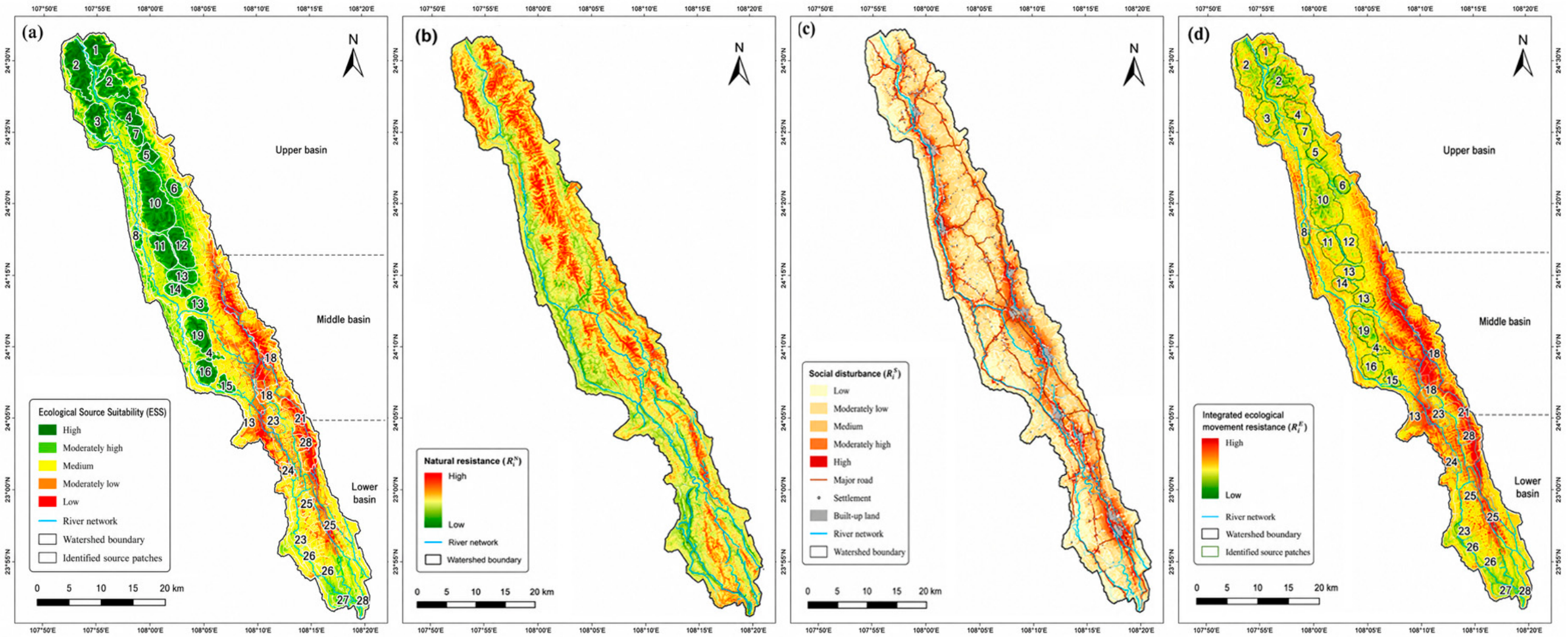
Under the baseline 1.5 km2 minimum core-source threshold, 28 ecological source patches were identified, covering 312.4 km2 or 24.4% of the basin. The upper basin contained the largest and most continuous sources (154.8 km2; 49.6% of total source area), while middle- and lower-basin sources were smaller and more dependent on riparian, wetland-margin, and slope–valley positions. Eleven source patches recorded dPC values of at least 10%, including several middle-basin patches located between upland sources, tributaries, and the river corridor. The spatial configuration and connectivity contributions of the ecological source patches are summarised in Table 4.
Resistance surfaces showed low values in continuous forest, wetland, and riparian vegetation and high values on exposed karst surfaces, quarry-affected slopes, construction margins, roads, settlements, fragmented cropland, and discontinuous riparian sections. Fine-scale social-disturbance contrasts were generated primarily by road density and settlement proximity; whereas, township-level population and GDP contributed broader inter-township gradients (Figure 2).

3.2. Potential Corridor Network and Bottleneck Diagnosis

Under the 20 km baseline source-pair distance, 76 potential connections were retained, forming a 243.1 km network dominated by longitudinal connections along the Chengjiang River and its tributaries. The upper basin retained broader low-cost connections; whereas, middle- and lower-basin routes were narrower and more dependent on riparian and stepping-stone habitats. Standardised MCR values classified the network into 22 primary, 33 secondary, and 21 tertiary corridors. Primary corridors mainly linked adjacent forest and headwater sources; secondary corridors connected riparian and slope–valley transitions; and tertiary corridors were generally narrower, more resistant, and more exposed to cropland, settlements, roads, and discontinuous riparian vegetation (Table 5).
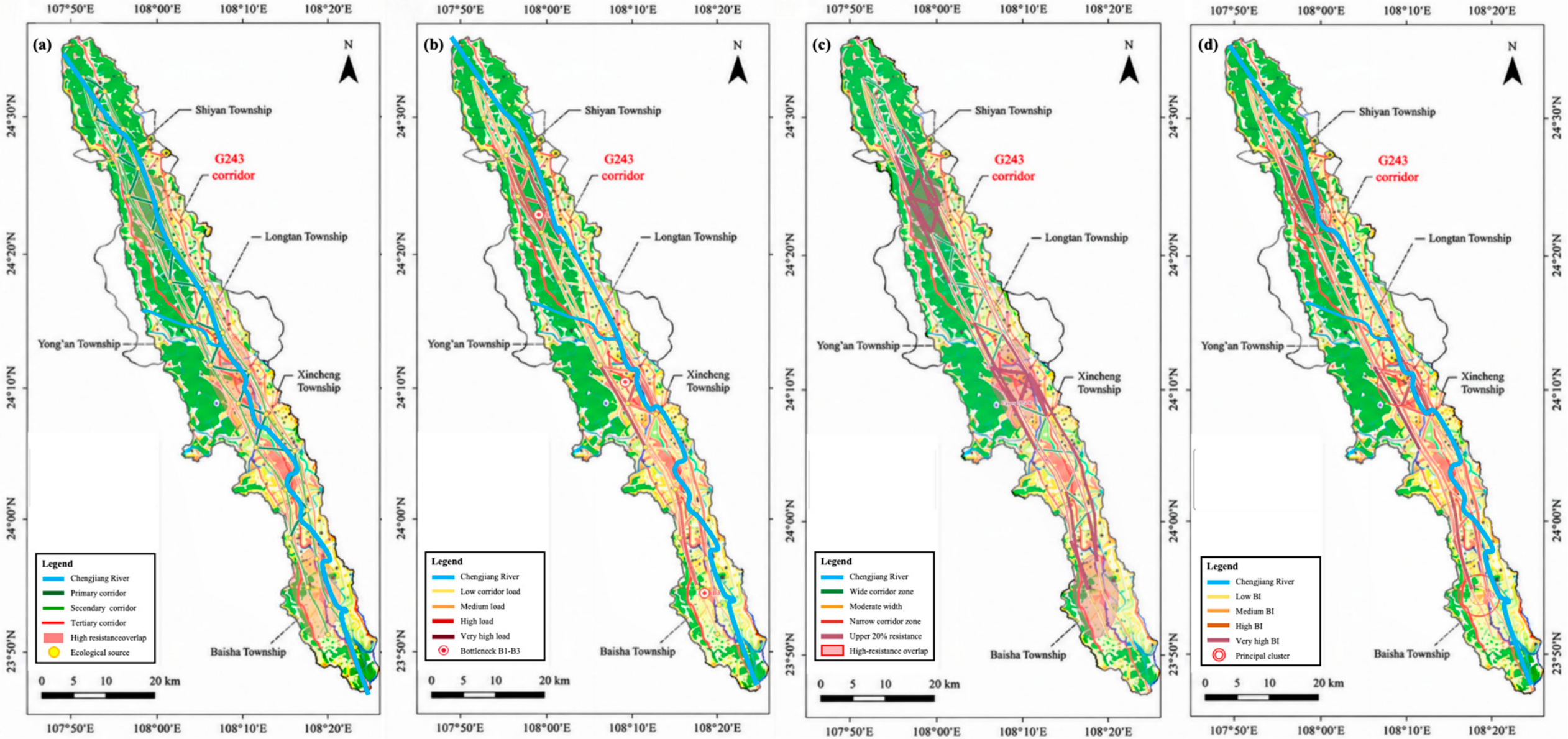
The baseline network yielded IIC = 0.212 and PC = 0.437. Combining corridor load, minimum width, and high-resistance overlap identified three bottleneck clusters: B1, a terrain- and quarry-related constriction in the upper-middle basin; B2, a road–riparian crossing bottleneck; and B3, a valley-matrix bottleneck associated with agriculture, settlement expansion, and riparian discontinuity (Figure 3).

3.3. Ecological Restoration Priority Zones and Governance Implementation Contexts

The Restoration Priority Index showed a spatially clustered distribution across the Chengjiang River Basin. Higher values occurred where elevated ecological movement resistance coincided with structurally vulnerable corridor sections, particularly around degraded source margins, quarry-affected slopes, road–river intersections, narrow riparian passages, settlement and construction edges, and fragmented agricultural valleys. Lower values were concentrated mainly in continuous forest, relatively intact riparian vegetation, and wider corridor sections with comparatively low resistance and Bottleneck Intensity. The continuous RPI surface was classified into low-, moderate-, and high-priority levels using Jenks natural breaks. After isolated fragments without a clear relationship to the ecological network or an identifiable restoration constraint were removed, contiguous high-priority cells formed six ERPZs, labelled ERPZ-A to ERPZ-F (Table 6). The zones covered approximately 118.5 km2, equivalent to 9.3% of the basin area, and were concentrated mainly in the middle and lower basin.
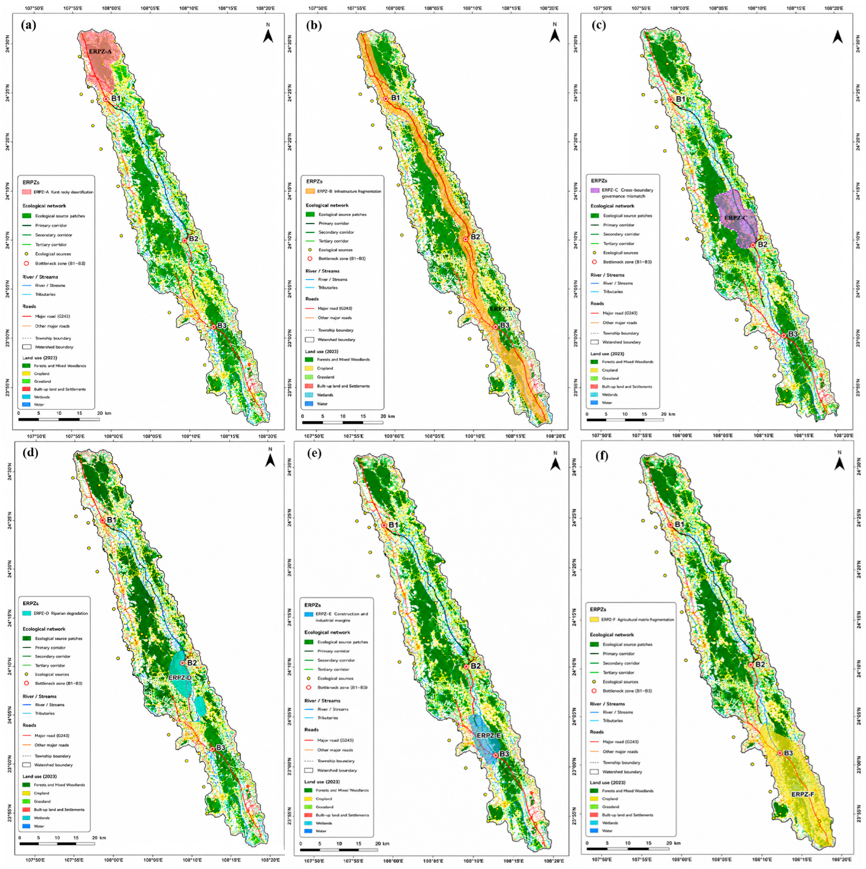
The six zones differed in their ecological mechanisms and their implementation conditions (Figure 4). ERPZ-level GMI values ranged from 0.57 to 0.72, with a median of 0.65. ERPZ-D recorded the highest GMI, followed by ERPZ-B and ERPZ-F, with comparatively greater mismatch among policy coordination, fiscal alignment, and cooperation capacity. These values described relative implementation conditions and did not contribute to ecological movement resistance, BI, RPI, or ERPZ delineation. ERPZ-level ABPI values ranged from 0.58 to 0.86. ERPZ-B had the highest boundary-proximity value, followed by ERPZ-E and ERPZ-C, indicating greater spatial exposure to township boundaries. ERPZ-A had the lowest ABPI and was more concentrated within a single administrative context. ABPI represented proximity to an administrative interface rather than evidence of administrative conflict or implementation failure. Using the respective ERPZ-level medians of GMI and ABPI as case-specific thresholds, ERPZ-A was classified as a local-implementation context. ERPZ-D and ERPZ-F were classified as institutional reinforcement contexts because their GMI values were comparatively high while their boundary exposure remained lower. ERPZ-C and ERPZ-E were classified as cross-boundary coordination contexts because of their higher ABPI but comparatively lower GMI. ERPZ-B was the only compound-coordination context, combining above-median governance mismatch with the highest administrative-boundary exposure. Using the ERPZ-level median GMI and ABPI values as case-specific thresholds, ERPZ-A was classified as a local-implementation context; ERPZ-D and ERPZ-F as institutional-reinforcement contexts; ERPZ-C and ERPZ-E as cross boundary coordination contexts; and ERPZ-B as a compound-coordination context. GMI and ABPI were applied after ERPZ delineation and did not alter the RPI surface, ERPZ boundaries, ecological-priority rankings, or priority-type classifications. The governance assessment did not modify the RPI surface, ERPZ boundaries, ecological-priority rankings, or resistance-, bottleneck-, and compound-priority classifications.

3.4. Validation and Sensitivity Results

The 2023 land-cover classification achieved an overall accuracy of 0.896 and a Cohen’s kappa coefficient of 0.874 based on 230 independent validation samples. The 1000 stratified bootstrap resamples produced bootstrap-based 95% confidence intervals of 0.852–0.935 for overall accuracy and 0.821–0.921 for Cohen’s kappa, the validation and spatial-stability results are summarised in Table 7. The complete year-specific confusion matrices for 2018–2023 are provided in Figure S1. The 2018–2022 matrices document the temporal consistency of the classification workflow; whereas, only the 2023 land-cover map was used as a direct input to the SRCG analysis.
The validation and sensitivity analyses showed comparatively stable basin-scale patterns for the ecological-source system, principal corridor structure, B1–B3 bottleneck clusters, and ERPZ cores. Sensitivity was greatest along corridor and ERPZ boundaries and within heterogeneous agricultural, settlement, and quarry-affected landscapes.

4. Discussion

4.1. Structural Connectivity and Bottleneck Mechanisms in a Karst Basin

Structural connectivity in the Chengjiang River Basin is maintained by the combined organisation of large habitat cores, strategically positioned connector patches, and a limited number of valley and riparian passages. The upstream–downstream gradient reflects the interaction between karst topography and valley-based land use. Relatively broad, low-cost connections occurred mainly in the forested upper basin, while the middle basin formed a structural transition zone in which several upland-to-river connections converged within landscapes affected by cropland, roads, settlements, and quarry disturbance. Lower-basin connectivity depended more strongly on fragmented riparian vegetation, wetland margins, and stepping-stone patches.
Primary corridors therefore represented the comparatively continuous network backbone; whereas, secondary and tertiary corridors were increasingly dependent on semi-permeable agricultural and settlement matrices. Because the corridor classes were derived from standardised MCR values and case-specific Jenks natural breaks, they represent relative conditions within the CRB rather than transferable ecological thresholds. The IIC and PC depend on source definition, network topology, and the adopted 20 km binary connection rule, their values should be interpreted as basin-specific indicators of potential structural connectivity rather than transferable ecological thresholds.
The Bottleneck Intensity analysis added a local diagnosis of structural vulnerability by integrating corridor load, minimum width, and high-resistance overlap. B1 represented terrain- and quarry-related constriction, B2 an infrastructure-crossing bottleneck at a road–riparian interface, and B3 a valley-matrix bottleneck associated with agricultural fragmentation, settlement expansion, and riparian discontinuity. Comparable studies have used pinch points, barrier areas, and network importance to identify critical restoration locations [9,12,15,18,19], while multi-temporal analysis has shown that the position and importance of network elements may change through time [17]. Nevertheless, corridor load represents modelled route convergence rather than animal abundance or movement frequency. MCR, IIC, PC, source-contribution indices, corridor width, and BI describe potential structural connectivity under the selected assumptions, not confirmed habitat use, dispersal, or gene flow [40,50,51,52,53]. The mapped network should therefore be interpreted as a basin-scale diagnosis of backbone connections, matrix-dependent pathways, and locally vulnerable passages requiring finer ecological assessment.

4.2. Differentiated Restoration Mechanisms of the ERPZs

The RPI addresses a complementary question by distinguishing whether ecological priority arises principally from extensive ecological movement resistance, localised Bottleneck Intensity, or their combined effects. This distinction reduces the limitations of single-factor prioritisation: resistance alone may emphasise broadly degraded areas with limited network relevance; whereas, BI alone may identify narrow passages without accounting for the surrounding landscape matrix. The six ERPZs represented three restoration mechanisms. ERPZ-A, ERPZ-D, ERPZ-E, and ERPZ-F were resistance-dominated, but their constraints differed: quarry and slope degradation in ERPZ-A, riparian and wetland-margin discontinuity in ERPZ-D, development-edge compression in ERPZ-E, and agricultural-matrix fragmentation in ERPZ-F. These zones require broader improvements in landscape permeability, including slope rehabilitation, riparian and wetland recovery, development-edge control, and reinforcement of field margins or stepping-stone habitats. ERPZ-B was bottleneck-dominated because several potential connections converged within a restricted road–riparian passage; restoration should therefore focus on continuity at the crossing and its adjacent riparian corridor. ERPZ-C was compound-priority and requires both matrix improvement and targeted reinforcement of constrained links.
These measures are planning directions rather than engineering prescriptions. Species-specific ecological validation remains necessary [50,51,52,53], while site-level hydrological, land-tenure, and transport-safety investigations are required before detailed design. ERPZs should therefore be treated as network-based diagnostic units rather than statutory control lines or final construction boundaries. Their central areas were more stable than peripheral cells, indicating that continuous RPI values, ecological-priority mechanisms, and field evidence should be considered jointly when intervention boundaries are refined. The three priority types remain relative classifications within the CRB and should not be transferred to other basins without recalibration.

4.3. Governance Implementation Contexts and Land-Governance Responses

The present study adopts a different analytical sequence: ecological priorities are delineated independently, after which GMI and ABPI are used to characterise the conditions under which restoration may be delivered. A high GMI indicates a relative mismatch among policy coordination, fiscal alignment, and cooperation capacity rather than governance failure, while a high ABPI indicates proximity to a township boundary rather than demonstrated administrative conflict. Neither index alters ecological movement resistance, corridor geometry, BI, RPI, ecological-priority type, or ERPZ boundaries. Implementation contexts show that similar ecological priorities may require different delivery arrangements (Table 8). ERPZ-E and ERPZ-F illustrate this distinction: both were resistance-dominated, but ERPZ-E had greater administrative-boundary exposure; whereas, ERPZ-F had greater governance mismatch. ERPZ-B combined a bottleneck-dominated ecological priority with above-median values for both GMI and ABPI. ERPZ-A was classified as a local-implementation context because both governance mismatch and boundary exposure were comparatively low. ERPZ-D and ERPZ-F required institutional reinforcement, indicating greater dependence on responsibility allocation, implementation continuity, compatible monitoring procedures, and long-term maintenance within the relevant administrative units. ERPZ-C and ERPZ-E were associated with cross-boundary coordination because restoration, monitoring, or maintenance may involve adjacent townships. ERPZ-B combined comparatively high governance mismatch with the highest boundary exposure and was classified as a compound-coordination context.
Implementation arrangements should correspond to these relative conditions. Local contexts may be organised through a clearly designated lead authority; institutional-reinforcement contexts require clearer responsibilities and more stable operational arrangements; cross-boundary contexts require coordinated schedules, land-use controls, and shared monitoring; and compound contexts may require county-level or interdepartmental coordination. Such responses are consistent with research on scale mismatch, institutional fit, cross-scale governance, collaborative environmental governance, and adaptive river-basin management [20,43,44,45,46,54,55]. However, the classifications were based on case-specific median thresholds for only six ERPZs and should not be interpreted as universal governance standards. The analysis also did not directly measure trust, leadership, enforcement, informal negotiation, community participation, budget execution, or actual interdepartmental performance. The proposed arrangements are therefore implementation hypotheses to be tested through interviews, administrative records, project documentation, and longitudinal evaluation rather than empirically demonstrated governance outcomes.

4.4. Methodological Contributions, Limitations, and Future Research

The SRCG framework makes three related contributions. First, it separates ecological-priority identification from governance implementation assessment while retaining both within one sequential planning framework, thereby avoiding the treatment of policy, fiscal, or administrative conditions as physical movement resistance. Second, BI extends conventional least-cost diagnosis by integrating route convergence, minimum corridor width, and high-resistance overlap, enabling the identification of connections that remain topologically present. Third, the framework distinguishes the ecological restoration mechanisms resistance-dominated, bottleneck-dominated, and compound-priority from the implementation contexts local implementation, institutional reinforcement, cross-boundary coordination, and compound coordination.
The methodological contributions, interpretation limitations, and future validation requirements of the SRCG framework are summarised in Table 9. Ecological network represents potential structural rather than functional connectivity, the 30 m grid provides a common analytical geometry but does not increase the native resolution of MODIS data or township-level socioeconomic and governance records. The resistance surface generalises ecological responses across species, while source thresholds, corridor tolerances, BI and RPI weights, and Jenks classifications remain parameter- and case-dependent. Deterministic sensitivity analysis showed that core sources, major corridors, B1–B3, and ERPZ centres were comparatively stable, but peripheral connections and zone boundaries were less certain. Bootstrap resampling quantified sampling uncertainty only for LULC classification accuracy; the study did not conduct full probabilistic propagation through all SRCG stages. Governance indicators were derived mainly from formal records and could not fully represent informal cooperation, institutional trust, participation, or actual implementation performance.
Future research should develop species- or functional-group-specific resistance surfaces and test corridor use through camera traps, acoustic monitoring, environmental DNA, telemetry, or landscape-genetic evidence. Multi-temporal and scenario-based analyses should examine whether the identified sources, bottlenecks, and ERPZs persist under land-use, infrastructure, restoration, and climate change. Recent ecological-network research has demonstrated that climate change and land-use/land-cover change may exert distinct and interactive effects on network structure and connectivity [8,15,17,21]. The present study did not model future climate scenarios or climate-driven changes in habitat suitability and should therefore be interpreted as a diagnosis of current potential structural connectivity. MCR outputs should also be compared with circuit theory, resistant-kernel, and individual-based models to assess alternative routes and network redundancy. Finally, implemented ERPZs should be monitored using ecological indicators, governance performance, and project-delivery evidence. More comprehensive ensemble or probabilistic sensitivity analysis may be introduced when defensible parameter distributions and sufficient input data become available. The SRCG framework should therefore be regarded as a basin-scale diagnostic and comparative prioritisation tool rather than a substitute for species-specific assessment, climate-adaptive scenario modelling, engineering design, financial appraisal, or direct evaluation of governance effectiveness.

5. Conclusions

This study developed a sequential SRCG framework for ecological-network diagnosis and restoration prioritisation in the Chengjiang River Basin. The framework separated ecological movement resistance from governance implementation conditions, thereby avoiding the treatment of administrative boundaries or institutional mismatch as ecological barriers. Twenty-eight ecological sources covering 312.4 km2 were identified. Large forest and headwater patches formed the principal habitat cores, while several smaller riparian and slope–valley sources made substantial contributions because of their connector positions. The 76 modelled source-pair connections formed a predominantly longitudinal network along the Chengjiang River and its tributaries. Primary corridors were generally wider and lower-cost; whereas, secondary and tertiary corridors were more dependent on fragmented agricultural, settlement, and riparian matrices. Three principal bottlenecks were associated with quarry and terrain related constriction, road–riparian interruption, and fragmented valley development.
By integrating normalised ecological movement resistance and Bottleneck Intensity, six ERPZs covering 118.5 km2 were delineated. ERPZ-A, ERPZ-D, ERPZ-E, and ERPZ-F were resistance-dominated, ERPZ-B was bottleneck-dominated, and ERPZ-C was compound-priority. These categories distinguished extensive reductions in landscape permeability from localised structural constriction and indicated that restoration strategies should be matched to the mechanism generating priority. The post hoc GMI–ABPI assessment further identified one local-implementation context, two institutional-reinforcement contexts, two cross-boundary coordination contexts, and one compound-coordination context. Governance indicators did not alter ecological-priority values, classifications, or ERPZ boundaries, but clarified the relative coordination and institutional requirements associated with implementation.
Validation and deterministic stability analyses provided qualified support for the basin-scale results. The land-cover classification achieved an overall accuracy of 0.896 and a Cohen’s kappa coefficient of 0.874, while 14 of 16 field-verification sections were consistent with the modelled landscape conditions. Source rankings, major corridors, bottleneck clusters, and ERPZ cores were comparatively stable, although corridor margins and ERPZ boundaries were more sensitive to parameter changes. The framework is therefore suitable for basin-scale structural-connectivity diagnosis and comparative restoration prioritisation. However, the outputs represent potential structural rather than demonstrated functional connectivity, and the governance indicators describe relative implementation contexts rather than observed institutional failure. Species-specific monitoring, finer-resolution spatial data, engineering assessment, and direct evaluation of restoration and governance outcomes are requireda before site-level intervention.

Supplementary Materials

The following supporting information can be downloaded at: https://www.mdpi.com/article/10.3390/land15081332/s1, Table S1: Key parameters, analytical decision rules, and sensitivity settings used in the SRCG framework; Figure S1: Year-specific Random Forest confusion matrices for the 2018–2023 land-use and land-cover classifications in the Chengjiang River Basin. The 2018–2022 matrices document the temporal consistency of the classification workflow; whereas, the 2023 matrix validates the land-cover map used directly for ecological-source identification, ecological movement-resistance modelling, corridor analysis, and ERPZ delineation. The earlier classifications were not used to infer historical land-use change or dynamic ecological-network evolution.

Author Contributions

Conceptualization, J.W. and B.L.; methodology, J.W.; software, J.W.; data curation, J.W.; formal analysis, J.W.; investigation, J.W.; visualisation, J.W.; writing—original draft preparation, J.W.; writing—review and editing, J.S. and J.W.; supervision, B.L.; project administration, B.L. All authors have read and agreed to the published version of the manuscript.

Funding

This research received no external funding.

Data Availability Statement

The original contributions presented in the study are included in the article/Supplementary Materials. Further inquiries can be directed to the corresponding author.

Conflicts of Interest

The authors declare no conflicts of interest.

References

  1. Ford, D.; Williams, P. Karst Hydrogeology and Geomorphology; John Wiley and Sons: Chichester, UK, 2007. [Google Scholar] [CrossRef] [Scilit]
  2. Jiang, Z.C.; Lian, Y.Q.; Qin, X.Q. Rocky desertification in Southwest China: Impacts, causes, and restoration. Earth-Sci. Rev. 2014, 132, 1–12. [Google Scholar] [CrossRef] [Scilit]
  3. Tong, X.; Brandt, M.; Yue, Y.; Horion, S.; Wang, K.; de Keersmaecker, W.; Tian, F.; Schurgers, G.; Xiao, X.; Luo, Y.; et al. Increased vegetation growth and carbon stock in China karst via ecological engineering. Nat. Sustain. 2018, 1, 44–50. [Google Scholar] [CrossRef] [Scilit]
  4. Pascual-Hortal, L.; Saura, S. Comparison and development of new graph-based landscape connectivity indices: Towards the priorization of habitat patches and corridors for conservation. Landsc. Ecol. 2006, 21, 959–967. [Google Scholar] [CrossRef] [Scilit]
  5. Saura, S.; Pascual-Hortal, L. A new habitat availability index to integrate connectivity in landscape conservation planning: Comparison with existing indices and application to a case study. Landsc. Urban Plan. 2007, 83, 91–103. [Google Scholar] [CrossRef] [Scilit]
  6. McRae, B.H.; Dickson, B.G.; Keitt, T.H.; Shah, V.B. Using circuit theory to model connectivity in ecology, evolution, and conservation. Ecology 2008, 89, 2712–2724. [Google Scholar] [CrossRef] [Scilit] [PubMed]
  7. Zeller, K.A.; McGarigal, K.; Whiteley, A.R. Estimating landscape resistance to movement: A review. Landsc. Ecol. 2012, 27, 777–797. [Google Scholar] [CrossRef] [Scilit]
  8. Li, Z.-T.; Li, M.; Xia, B.-C. Spatio-temporal dynamics of ecological security pattern of the Pearl River Delta urban agglomeration based on LUCC simulation. Ecol. Indic. 2020, 114, 106319. [Google Scholar] [CrossRef] [Scilit]
  9. Jiang, H.; Peng, J.; Zhao, Y.; Xu, D.; Dong, J. Zoning for ecosystem restoration based on ecological network in mountainous region. Ecol. Indic. 2022, 142, 109138. [Google Scholar] [CrossRef] [Scilit]
  10. Gao, M.; Hu, Y.; Bai, Y. Construction of ecological security pattern in national land space from the perspective of the community of life in mountain, water, forest, field, lake and grass: A case study in Guangxi Hechi, China. Ecol. Indic. 2022, 139, 108867. [Google Scholar] [CrossRef] [Scilit]
  11. Zhang, Y.; Zhao, Z.; Fu, B.; Ma, R.; Yang, Y.; Lü, Y.; Wu, X. Identifying ecological security patterns based on the supply, demand and sensitivity of ecosystem service: A case study in the Yellow River Basin, China. J. Environ. Manag. 2022, 315, 115158. [Google Scholar] [CrossRef] [Scilit] [PubMed]
  12. Gao, C.; Pan, H.; Wang, M.; Zhang, T.; He, Y.; Cheng, J.; Yao, C. Identifying priority areas for ecological conservation and restoration based on circuit theory and dynamic weighted complex network: A case study of the Sichuan Basin. Ecol. Indic. 2023, 155, 111064. [Google Scholar] [CrossRef] [Scilit]
  13. Dong, X.; Wang, F.; Fu, M. Research progress and prospects for constructing ecological security pattern based on ecological network. Ecol. Indic. 2024, 168, 112800. [Google Scholar] [CrossRef] [Scilit]
  14. Yang, M.; He, J.; Shi, L.; Lv, Y.; Li, J. Integrating policy quantification analysis into ecological security pattern construction: A case study of Guangdong–Hong Kong–Macao Greater Bay Area. Ecol. Indic. 2024, 162, 112049. [Google Scholar] [CrossRef] [Scilit]
  15. Ma, B.; Zeng, C.; Lv, T.; Liu, W.; Yang, W. prioritisation of ecological conservation and restoration areas through ecological networks: A case study of Nanchang City, China. Land 2024, 13, 878. [Google Scholar] [CrossRef] [Scilit]
  16. Zhang, R.; Li, H.; Liu, Z. Synergistic enhancement of carbon sinks and connectivity: Restoration and renewal of ecological networks in Nanjing, China. Land 2025, 14, 93. [Google Scholar] [CrossRef] [Scilit]
  17. Su, J.; Wu, M.; Liu, Z. Spatial–temporal evolution of ecological network structure during 1967–2021 in Yongding River Floodplain. Land 2025, 14, 930. [Google Scholar] [CrossRef] [Scilit]
  18. Zhang, W.; Fan, Y.; Qiao, Q.; Shao, G.; Zhang, M.; Lei, S.; Han, Y. Delineating ecological restoration zoning integrating functional and structural models in Horqin Sandy Land, China. Forests 2025, 16, 1616. [Google Scholar] [CrossRef] [Scilit]
  19. Yan, S.; Zhang, X.; Yan, R.; Luo, Y.; Wang, H.; Xing, B.; Liu, C.; Xu, D.; Liao, G. Identification of ecological restoration zones based on ecological security pattern and ecological risk assessment—A case study of Liaoning Province. Sustainability 2026, 18, 204. [Google Scholar] [CrossRef] [Scilit]
  20. Cumming, G.S.; Cumming, D.H.M.; Redman, C.L. Scale mismatches in social-ecological systems: Causes, consequences, and solutions. Ecol. Soc. 2006, 11, 14. [Google Scholar] [CrossRef] [Scilit]
  21. Ren, J.; Wang, W.J.; Fei, L.; Wang, L.; Xing, S.; Cong, Y. Impacts of climate change and land use/cover change on ecological security networks in Changbai Mountains, Northeast China. Ecol. Indic. 2024, 169, 112849. [Google Scholar] [CrossRef] [Scilit]
  22. Turner, M.G.; O’Neill, R.V.; Gardner, R.H.; Milne, B.T. Effects of changing spatial scale on the analysis of landscape pattern. Landsc. Ecol. 1989, 3, 153–162. [Google Scholar] [CrossRef] [Scilit]
  23. Main-Knorn, M.; Pflug, B.; Louis, J.; Debaecker, V.; Müller-Wilm, U.; Gascon, F. Sen2Cor for Sentinel-2. In Image and Signal Processing for Remote Sensing XXIII; SPIE: Bellingham, WA, USA, 2017; Volume 10427, p. 1042704. [Google Scholar] [CrossRef] [Scilit]
  24. Soenen, S.A.; Peddle, D.R.; Coburn, C.A. SCS+C: A modified sun-canopy-sensor topographic correction in forested terrain. IEEE Trans. Geosci. Remote Sens. 2005, 43, 2148–2159. [Google Scholar] [CrossRef] [Scilit]
  25. Breiman, L. Random forests. Mach. Learn. 2001, 45, 5–32. [Google Scholar] [CrossRef] [Scilit]
  26. Cutler, D.R.; Edwards, T.C., Jr.; Beard, K.H.; Cutler, A.; Hess, K.T.; Gibson, J.; Lawler, J.J. Random forests for classification in ecology. Ecology 2007, 88, 2783–2792. [Google Scholar] [CrossRef] [Scilit] [PubMed]
  27. Congalton, R.G. A review of assessing the accuracy of classifications of remotely sensed data. Remote Sens. Environ. 1991, 37, 35–46. [Google Scholar] [CrossRef] [Scilit]
  28. Foody, G.M. Status of land cover classification accuracy assessment. Remote Sens. Environ. 2002, 80, 185–201. [Google Scholar] [CrossRef] [Scilit]
  29. Tucker, C.J. Red and photographic infrared linear combinations for monitoring vegetation. Remote Sens. Environ. 1979, 8, 127–150. [Google Scholar] [CrossRef] [Scilit]
  30. Huete, A.; Didan, K.; Miura, T.; Rodriguez, E.P.; Gao, X.; Ferreira, L.G. Overview of the radiometric and biophysical performance of the MODIS vegetation indices. Remote Sens. Environ. 2002, 83, 195–213. [Google Scholar] [CrossRef] [Scilit]
  31. Savitzky, A.; Golay, M.J.E. Smoothing and differentiation of data by simplified least squares procedures. Anal. Chem. 1964, 36, 1627–1639. [Google Scholar] [CrossRef] [Scilit]
  32. Farr, T.G.; Rosen, P.A.; Caro, E.; Crippen, R.; Duren, R.; Hensley, S.; Kobrick, M.; Paller, M.; Rodriguez, E.; Roth, L.; et al. The Shuttle Radar Topography Mission. Rev. Geophys. 2007, 45, RG2004. [Google Scholar] [CrossRef] [Scilit]
  33. Bazeley, P.; Jackson, K. Qualitative Data Analysis with NVivo, 2nd ed.; SAGE Publications: London, UK, 2013. [Google Scholar]
  34. Cohen, J. A coefficient of agreement for nominal scales. Educ. Psychol. Meas. 1960, 20, 37–46. [Google Scholar] [CrossRef] [Scilit]
  35. Sharp, R.; Douglass, J.; Wolny, S.; Arkema, K.; Bernhardt, J.; Bierbower, W.; Chaumont, N.; Denu, D.; Fisher, D.; Glowinski, K.; et al. InVEST 3.9.0 User’s Guide; The Natural Capital Project: Stanford, CA, USA, 2020. [Google Scholar]
  36. McGarigal, K.; Marks, B.J. FRAGSTATS: Spatial Pattern Analysis Program for Quantifying Landscape Structure; General Technical Report PNW-GTR-351; USDA Forest Service, Pacific Northwest Research Station: Portland, OR, USA, 1995. [CrossRef] [Scilit]
  37. Naiman, R.J.; Décamps, H. The ecology of interfaces: Riparian zones. Annu. Rev. Ecol. Syst. 1997, 28, 621–658. [Google Scholar] [CrossRef] [Scilit]
  38. Adriaensen, F.; Chardon, J.P.; de Blust, G.; Swinnen, E.; Villalba, S.; Gulinck, H.; Matthysen, E. The application of least-cost modelling as a functional landscape model. Landsc. Urban Plan. 2003, 64, 233–247. [Google Scholar] [CrossRef] [Scilit]
  39. Yu, K.J. Security patterns and surface model in landscape ecological planning. Landsc. Urban Plan. 1996, 36, 1–17. [Google Scholar] [CrossRef] [Scilit]
  40. Beier, P.; Majka, D.R.; Spencer, W.D. Forks in the road: Choices in procedures for designing wildland linkages. Conserv. Biol. 2008, 22, 836–851. [Google Scholar] [CrossRef] [Scilit] [PubMed]
  41. Spear, S.F.; Balkenhol, N.; Fortin, M.J.; McRae, B.H.; Scribner, K. Use of resistance surfaces for landscape genetic studies: Considerations for parameterization and analysis. Mol. Ecol. 2010, 19, 3576–3591. [Google Scholar] [CrossRef] [Scilit] [PubMed]
  42. Saura, S.; Torné, J. Conefor Sensinode 2.2: A software package for quantifying the importance of habitat patches for landscape connectivity. Environ. Model. Softw. 2009, 24, 135–139. [Google Scholar] [CrossRef] [Scilit]
  43. Moss, T. Spatial fit, from panacea to practice: Implementing the EU Water Framework Directive. Ecol. Soc. 2012, 17, 2. [Google Scholar] [CrossRef] [Scilit]
  44. Young, O.R. The Institutional Dimensions of Environmental Change: Fit, Interplay, and Scale; MIT Press: Cambridge, MA, USA, 2002. [Google Scholar] [CrossRef] [Scilit]
  45. Cash, D.W.; Adger, W.N.; Berkes, F.; Garden, P.; Lebel, L.; Olsson, P.; Pritchard, L.; Young, O. Scale and cross-scale dynamics: Governance and information in a multilevel world. Ecol. Soc. 2006, 11, 8. [Google Scholar] [CrossRef] [Scilit]
  46. Epstein, G.; Pittman, J.; Alexander, S.M.; Berdej, S.; Dyck, T.; Kreitmair, U.; Rathwell, K.J.; Villamayor-Tomas, S.; Vogt, J.; Armitage, D. Institutional fit and the sustainability of social-ecological systems. Curr. Opin. Environ. Sustain. 2015, 14, 34–40. [Google Scholar] [CrossRef] [Scilit]
  47. Efron, B.; Tibshirani, R.J. An Introduction to the Bootstrap; Chapman & Hall/CRC: New York, NY, USA, 1993. [Google Scholar] [CrossRef] [Scilit]
  48. Saltelli, A.; Tarantola, S.; Campolongo, F.; Ratto, M. Sensitivity Analysis in Practice: A Guide to Assessing Scientific Models; John Wiley and Sons: Chichester, UK, 2004. [Google Scholar] [CrossRef] [Scilit]
  49. Jaccard, P. The distribution of the flora in the alpine zone. New Phytol. 1912, 11, 37–50. [Google Scholar] [CrossRef] [Scilit]
  50. Tischendorf, L.; Fahrig, L. On the usage and measurement of landscape connectivity. Oikos 2000, 90, 7–19. [Google Scholar] [CrossRef] [Scilit]
  51. Baguette, M.; van Dyck, H. Landscape connectivity and animal behavior: Functional grain as a key determinant for dispersal. Landsc. Ecol. 2007, 22, 1117–1129. [Google Scholar] [CrossRef] [Scilit]
  52. Keeley, A.T.H.; Beier, P.; Keeley, B.W.; Fagan, M.E. Habitat suitability is a poor proxy for landscape connectivity during dispersal and mating movements. Landsc. Urban Plan. 2017, 161, 90–102. [Google Scholar] [CrossRef] [Scilit]
  53. Chetkiewicz, C.L.B.; St. Clair, C.C.; Boyce, M.S. Corridors for conservation: Integrating pattern and process. Annu. Rev. Ecol. Evol. Syst. 2006, 37, 317–342. [Google Scholar] [CrossRef] [Scilit]
  54. Bodin, Ö. Collaborative environmental governance: Achieving collective action in social-ecological systems. Science 2017, 357, eaan1114. [Google Scholar] [CrossRef] [Scilit] [PubMed]
  55. Pahl-Wostl, C.; Lebel, L.; Knieper, C.; Nikitina, E. From applying panaceas to mastering complexity: Toward adaptive water governance in river basins. Environ. Sci. Policy 2012, 23, 24–34. [Google Scholar] [CrossRef] [Scilit]
Figure 1. Location and environmental setting of the Chengjiang River Basin: (a) nested regional location from China to Guangxi Zhuang Autonomous Region, Du’an Yao Autonomous County, and the CRB, with red outlines indicating the next nested spatial unit; (b) elevation classes, the main river, tributaries, township boundaries, and the basin boundary; and (c) 2023 land-use and land-cover classes, major and secondary roads, settlements, township boundaries, and the basin boundary.
Land 15 01332 g001
Figure 2. Spatial patterns of ecological sources and ecological movement resistance in the CRB: (a) Ecological source suitability and the 28 identified source patches, with numbered labels denoting individual source patches; (b) Natural resistance; (c) Social disturbance; and (d) Integrated ecological movement resistance. Grey dashed lines in panels (a,d) indicate the descriptive Upper, Middle, and Lower basin divisions.
Land 15 01332 g002
Figure 3. Potential ecological corridor network and bottleneck patterns in the CRB: (a) primary, secondary, and tertiary corridors classified from the basin-specific distribution of standardised pairwise MCR values; (b) corridor load derived from overlapping source-pair corridor zones; (c) minimum corridor-zone width and overlap with the upper 20% of ecological movement resistance; (d) Bottleneck Intensity and the principal bottleneck clusters B1–B3.
Land 15 01332 g003
Figure 4. ERPZs and governance implementation contexts in the CRB: (a) ERPZ-A: mining and slope disturbance; (b) ERPZ-B: road interruption; (c) ERPZ-C: fragmented valley matrix and convergent ecological connections; (d) ERPZ-D: riparian degradation; (e) ERPZ-E: construction and industrial margins; (f) ERPZ-F: agricultural matrix fragmentation. Each panel shows the spatial relationship between the selected ERPZ, ecological corridors, source patches, bottleneck zones, and the surrounding land-use matrix.
Land 15 01332 g004
Table 1. Data sources and analytical applications in the Chengjiang River Basin.
Data TypeVariablesData Source
and Period
Spatial Resolution/ScaleAnalytical Application
Land use and land coverForest and mixed woodland; cropland; grassland and shrubland; built-up land and settlements; bare rock and sparsely vegetated land; wetland; waterLandsat 8 and Sentinel-2 L2A imagery, 202310–30 mLand-cover classification, habitat-quality assessment, ecological source identification, and resistance assignment
Classification samplesLand-cover reference samples distributed across land-cover classes, basin sections, and terrain settingsHigh-resolution reference imagery and field observations, 2023–2024Sample pointsRandom Forest training and independent validation; 1200 training samples and 230 validation samples
Vegetation conditionNDVI and EVIMODIS MOD13Q1, 2000–2023250 mLong-term vegetation vitality and ecological source screening
TopographyElevation, slope, curvature, and topographic wetness indexSRTM v3; ASTER GDEM used for terrain-pattern checking30 mTerrain analysis and natural resistance
Karst lithology and geologyCarbonate-rock type, limestone and dolomite distribution, non-carbonate geological units, and structural featuresGLiM v1.0 and Guangxi regional geological mapsPolygon data; regional maps at approximately 1:50,000–1:250,000Lithological resistance and interpretation of karst sensitivity
Soil erosion and rocky desertificationSoil-erosion intensity, erosion risk, bare-rock exposure, and rocky-desertification tendencyRUSLE-based erosion assessment using 2023 environmental inputs and supporting erosion data30 m after harmonisationErosion-related resistance and high-resistance interpretation
Hydrology and wetlandsMain river, tributaries, perennial water bodies, wetlands, and riparian zonesOfficial hydrological records and remote-sensing interpretationVector and rasterHydrological proximity, source identification, and corridor interpretation
Infrastructure and settlementsRoads, transport crossings, settlements, construction land, and quarry-affected areasOpenStreetMap, high-resolution imagery, and field correction, 2022–2024Vector and classified rasterLocalised anthropogenic disturbance and interpretation of corridor constraints
Socioeconomic conditionsPopulation and GDPGuangxi statistical yearbooks and township statistics, 2023TownshipBroad socioeconomic-pressure gradients within the social-disturbance component and contextual interpretation of restoration implementation
Governance and administrative dataPolicy coordination, fiscal and ecological-compensation support, joint monitoring, inter-township cooperation, and township boundariesDu’an County and township records, 2018–2024Text, township, and vectorGMI, ABPI, and ERPZ implementation-context assessment
Field observationsLand cover, vegetation continuity, riparian condition, corridor constriction, transport disturbance, exposed slopes, and quarry disturbanceField surveys, May–August 2024Points and corridor sectionsLand-cover validation and landscape-condition verification
Table 2. Governance indicators used to assess restoration implementation conditions.
DimensionOperational IndicatorCalculation and NormalisationNative Spatial ScaleAnalytical Role And Interpretation
Policy coordinationProportion of relevant clauses addressing coordinated restorationRelevant coded provisions divided by all included provisions and normalised to 0–1TownshipMeasures formal policy alignment and constitutes P j in the GMI
Fiscal alignmentCorrespondence between restoration responsibilities and available fiscal or ecological-compensation supportResponsibility–support correspondence transformed into an adequacy score and normalised to 0–1TownshipMeasures alignment between restoration responsibility and fiscal support and constitutes F j in the GMI
Cooperation frequencyRecorded joint meetings, shared monitoring, coordinated projects, and inter-township activitiesJoint meetings, shared monitoring, inter-township coordination, and cross-boundary projects; normalised to 0–1TownshipMeasures operational capacity for joint implementation and constitutes C j in the GMI
Administrative boundary proximityDistance to the nearest township boundary ABPI i = e x p ( d i λ ) where d i is the distance from grid cell i to the nearest township boundary and λ is the distance-decay parameter.Grid summarised by ERPZIdentifies ERPZs with greater potential demand for cross-boundary coordination
Table 3. Key parameters and analytical decision rules used in the SRCG framework.
Analytical ComponentBaseline SettingAlternative SettingsStability Output
Minimum ecological-source area1.5 km21.2 and 1.8 km2Source number, total source area, spatial overlap, dPC and dIIC rankings
Natural/social resistance ratio0.643/0.3570.50/0.50, 0.60/0.40, and 0.70/0.30Resistance-surface correlation, corridor configuration, bottleneck retention, and ERPZ overlap
Maximum source-pair distance20 km16 and 24 kmRetained source pairs, corridor number and length, IIC, PC, dPC, and dIIC
Relative excess-cost tolerance0.050.04 and 0.06Corridor-zone area, width, class retention, and Jaccard similarity
High-resistance thresholdUpper 20% of the basin-wide resistance distributionUpper 15% and upper 25%High-resistance overlap, BI rankings, and retention of B1–B3
BI component weightsCorridor load/minimum width/high-resistance overlap = 0.40/0.35/0.25Each component perturbed by ±10% and ±20%, followed by renormalisationSegment-level BI rankings and retention of principal bottlenecks
RPI component weightsEcological movement resistance/BI = 0.57/0.430.50/0.50, 0.60/0.40, and 0.70/0.30RPI rankings, ERPZ number and area, Jaccard similarity, and ecological-priority type
GMI constructionEqual weights of 1/3 for policy coordination, fiscal alignment, and cooperation frequencyThree component-dominant weighting scenarios and geometric aggregationERPZ-level GMI rankings and implementation-context classification
ABPI distance-decay parameter500 m400 and 600 mERPZ-level ABPI rankings and implementation-context classification
Table 4. Spatial configuration and connectivity contribution of ecological source patches in the CRB.
Basin SectionNumber of SourcesTotal Source Area (km2)Share of Total Source Area (%)Mean Source Area (km2)Mean dPC (%)Key Sources dPC     10 % Highest dPC / dIIC SourceHighest dPC / dIIC (%)Spatial Characteristics
Upper basin11154.849.614.078.85ES-01, ES-02 ES-03, ES-04ES-0117.6/16.1Large forest and headwater cores; contribution primarily associated with habitat area and flux
Middle basin10112.536.011.2511.39ES-12, ES-13
ES-14, ES-16 ES-17, ES-18
ES-1619.2/16.8Heterogeneous valley sources with strong riparian and slope–valley connector functions
Lower basin745.114.46.447.29ES-24ES-2412.4/10.6Smaller fragmented sources with localised wetland-margin connector importance
Entire basin28312.4100.011.169.3711 sourcesES-1619.2/16.8Basin-wide connectivity maintained jointly by large habitat cores and intermediate connector patches
Table 5. Quantitative characteristics of potential ecological corridors in the CRB.
Corridor ClassNumber of Connections (%)Total Centreline Length, km (%)Standardised MCR, Median (IQR)Minimum Width, m, Median (IQR)High-Resistance Overlap, %, Median (IQR)Bottleneck Intensity, Median (IQR)
Primary22 (28.9)86.9 (35.7)0.17 (0.09–0.26)286 (205–392)8.6 (5.1–13.4)0.26 (0.18–0.34)
Secondary33 (43.4)93.4 (38.4)0.48 (0.37–0.59)164 (112–236)21.7 (15.2–29.8)0.52 (0.42–0.62)
Tertiary21 (27.6)62.8 (25.8)0.81 (0.70–0.91)76 (48–118)42.6 (33.5–52.8)0.79 (0.68–0.88)
Entire network76 (100.0)243.1 (100.0)
Table 6. Ecological characteristics and governance implementation contexts of the ERPZs in the CRB.
ERPZBasin SectionDominant Ecological ConstraintEcological Priority TypeArea (km2) R E BIRPIGMIABPI
ERPZ-AUpper middleQuarry disturbance, exposed karst slopes, vegetation degradation, and erosion-prone source marginsResistance dominated24.80.740.620.690.610.58
ERPZ-BMiddleRoad–riparian interruption, corridor convergence, and localised corridor-zone narrowingBottleneck dominated13.60.630.840.720.680.86
ERPZ-CMiddleConnector discontinuity and multiple corridor convergence within a fragmented valley matrixCompound priority20.70.680.780.720.640.74
ERPZ-DMiddle lowerRiparian discontinuity, wetland-margin degradation, and restricted longitudinal connectivityResistance18.40.600.730.660.720.69
ERPZ-ELowerConstruction-, settlement-, and industrial-edge compression of riparian and wetland-associated connectionsResistance16.90.720.650.690.570.82
ERPZ-FMiddle lowerAgricultural-matrix fragmentation, rural-road disturbance, and discontinuous field-margin and stepping-stone habitatsResistance24.10.660.580.630.660.63
Total or median118.50.650.72
Table 7. Validation and spatial-stability results for the ecological network and restoration-priority model.
Assessment
Component
Validation or Scenario BasisMetricInterpretation
Land-cover classification230 independent validation samplesOverall accuracy0.896; 95%
CI: 0.852–0.935
Land-cover classification230 independent validation samplesCohen’s kappa0.874; 95%
CI: 0.821–0.921
Field verification16 representative corridor sectionsConsistent sections14 of 16 (87.5%)
Corridor-zone stabilityAlternative source, resistance, corridor, and BI settingsJaccard similarity0.760–0.936
ERPZ stabilityAlternative resistance–BI weights and corridor settings0.851–0.953
Source-ranking stabilityAlternative source and resistance settingsSpearman correlation of dPC 0.986–1.000
Spearman correlation of dIIC 0.993–0.999
Bottleneck stabilityAlternative resistance thresholds and BI weightsPrincipal-cluster retentionB1–B3 retained
Governance sensitivityAlternative GMI weights and ABPI decay parametersImplementation context stabilityChanges concentrated near median thresholds
Table 8. Governance implementation contexts and indicative coordination considerations for the ERPZs.
Implementation ContextERPZsMain Implementation IssueIndicative Coordination and Monitoring
Local implementationERPZ-ALow governance mismatch and limited boundary exposureDesignate a lead unit; monitor implementation, maintenance, vegetation recovery, and erosion control.
Institutional reinforcementERPZ-D, ERPZ-FHigher governance mismatch within the relevant administrative unitsClarify responsibilities and monitoring procedures; assess implementation continuity, riparian condition, and agricultural compatibility.
Cross-boundary coordinationERPZ-C, ERPZ-EHigh exposure to township boundariesCoordinate restoration timing, land-use controls, monitoring, and maintenance between adjacent townships.
Compound coordinationERPZ-BHigh governance mismatch and boundary exposure at a road–riparian bottleneckEstablish interdepartmental coordination; monitor responsibility fulfilment, crossing condition, riparian continuity, and maintenance.
Table 9. Methodological contributions, interpretation limitations, and future validation requirements of the SRCG framework.
Analytical ComponentContributionPrincipal LimitationFuture Validation
Sequential SRCG frameworkSeparates ecological-priority identification from governance implementation assessmentDoes not demonstrate causal relationships between governance conditions and ecological outcomesLongitudinal evaluation of implemented restoration projects
Source and graph analysisQuantifies habitat, flux, and connector importance using dPC and dIICResults depend on source definition and generalised connectivity assumptionsSpecies-specific habitat, occurrence, movement, or genetic data
Ecological movement resistanceIntegrates natural constraints and anthropogenic disturbance without governance variablesDoes not capture species- or season-specific responsesTaxon-specific and seasonal resistance models
MCR and BIIdentifies potential connections and local structural vulnerabilityModelled corridors and corridor load do not demonstrate actual movementCamera traps, acoustic surveys, tracking and landscape genetics
RPI and ERPZsDifferentiates resistance-, bottleneck-, and compound-priority mechanismsBoundaries depend on parameters and classification choicesFiner-resolution mapping and post-restoration monitoring
GMI–ABPI assessmentCharacterises institutional mismatch and boundary exposure after ecological zoningDoes not prove governance conflict or implementation failureInterviews, budgets, project records, and stakeholder analysis
Stability analysisTests consistency under deterministic parameter scenariosDoes not provide a full probabilistic uncertainty distributionReproducible GIS ensembles and formal uncertainty propagation
Disclaimer/Publisher’s Note: The statements, opinions and data contained in all publications are solely those of the individual author(s) and contributor(s) and not of MDPI and/or the editor(s). MDPI and/or the editor(s) disclaim responsibility for any injury to people or property resulting from any ideas, methods, instructions or products referred to in the content.