Spatiotemporal Evolution and Driving Mechanisms of Carbon–Water Coupling Coordination in the Dongping Lake Basin from 1990 to 2020

Abstract

The Dongping Lake Basin (DLB) serves as a critical water regulation and supply zone for the South-to-North Water Diversion Project in China. Understanding the coupling effects and influence mechanisms between ecosystem services is essential for regional ecological restoration and sustainable development. This study employed the Coupling Coordination Degree (CCD) model, Random Forest, and Geodetector. We analyzed the spatiotemporal characteristics and driving factors of the relationship between carbon storage and water yield in the DLB from 1990 to 2020. The results showed that: (1) Carbon storage and water yield exhibited a pronounced spatial mismatch. This was generally characterized by a pattern of high in the eastern/northeastern regions and low in the west/southwest. (2) The overall coordination between carbon storage and water yield remained at a medium-to-low level. Temporally, the CCD followed a trajectory of initial stability, abrupt decline post-2000, and subsequent low-level stagnation. Spatially, the CCD presented an agglomeration gradient of “high in the northeast and low in the southwest”. It also exhibited a significant positive correlation with rising elevation, peaking in mid-to-high altitude zones. Furthermore, the overall coupling relationship showed a continuous degradation trend, heavily concentrated in the southwestern region. (3) Land use type and topographic slope were the primary driving factors shaping the CCD pattern. However, the synergistic interaction between precipitation and soil sand content demonstrated the strongest spatial explanatory power. This underscores the necessity of adapting localized management to specific environmental conditions. This study provides scientific support for carbon sink enhancement and water resource management in lake basins, thereby mitigating potential negative impacts on human well-being.

1. Introduction

Watershed ecosystems are core components of the Earth’s critical zone. Maintaining and enhancing their carbon sequestration and water yield services is of global significance for addressing climate change and ensuring water security [1,2,3]. Under the dual pressures of global change and human activities, the interrelationships among ecosystem services have become increasingly complex. Consequently, understanding their synergistic and trade-off mechanisms has emerged as a frontier hotspot in geography and ecology [4,5]. Within the watershed “land–water” continuum, carbon sequestration and water yield are closely coupled [6]; Water supply provides the basis for photosynthetic carbon fixation, creating a fundamental carbon–water eco-geochemical link [7]; Conversely, vegetation fixes carbon dioxide and stores it in the soil, which improves soil structure, enhances infiltration, and boosts water-holding capacity, ultimately influencing runoff and groundwater recharge [6,7]. Concurrently, topography and hydrological gradients drive vegetation distribution, feeding back into the watershed’s ecological pattern through these coordination mechanisms [8].

Despite the importance of these highly dynamic carbon–water feedbacks, systematic quantitative assessments of their coupling degree remain scarce [9]. Globally, particularly in semi-arid and Mediterranean basins, extensive ecological restoration has exposed severe carbon–water trade-offs, where increased vegetation carbon sequestration is frequently offset by amplified evapotranspiration, thereby depleting regional water yield [10,11]. While these studies deepen our understanding of vegetation-climate feedbacks, macro-scale carbon–water coupling lacks systematic quantification [12]. Although some studies indicate that watershed carbon and water services may coordinate at large scales [13,14] while exhibiting opposite trends in plain areas, most research remains limited to qualitative descriptions. They frequently fail to reveal the spatiotemporal characteristics and the precise coordination degree of these coupling relationships [15,16]. Therefore, an urgent need exists for a macro-assessment framework capable of characterizing the coupling intensity and coordination state of carbon–water services to identify key regulatory areas.

To quantitatively assess these dependencies, the Coupling Coordination Degree (CCD) model is widely utilized [17,18]. However, current research applying this model often falls short in parsing the underlying driving mechanisms. Climate variables (e.g., precipitation, temperature), topography, and human activities not only independently affect hydrological and carbon cycles but also exhibit complex, non-linear interactive effects [19,20,21]. Substantial uncertainty remains regarding how these multifactorial interactions jointly modulate the coupling coordination of carbon–water services [22].

To address these critical gaps, this study focuses on the Dongping Lake Basin (DLB). As an ecological security barrier in the lower Yellow River and a vital regulation node for the South-to-North Water Diversion Project, the DLB faces severe pressures from wetland shrinkage and intense human-induced fragmentation [23,24]. We construct a comprehensive macro-assessment framework integrating the InVEST model, the CCD model, and Geodetector to reveal the spatiotemporal heterogeneity and dominant drivers of carbon–water coupling in the DLB from 1990 to 2020. The explicit marginal contributions of this study are threefold:

(1)

Methodological Paradigm Shift: We advance the analytical framework from isolated ecosystem service assessments to a dynamic, 30-year spatiotemporal continuum of carbon–water coupling coordination.

(2)

Mechanistic Insight: By integrating the CCD model with Geographic Detectors and Random Forest algorithms, we quantitatively unravel the non-linear interactive mechanisms between dynamic anthropogenic land-use boundaries and localized climate–soil conditions.

(3)

Practical Management Application: We translate abstract coupling metrics into spatially explicit, actionable ecological restoration strategies tailored to specific altitudinal and topographical zones, providing a robust decision-support tool for transitional basins globally.

Ultimately, the findings will provide a direct scientific basis for adaptive ecosystem management and the optimal allocation of resources in similar lake basins under the constraints of global climate change.

2. Study Area and Data

2.1. Study Area

The Dongping Lake Basin is located in the central-western part of Shandong Province, China (116°15′~117°59′ E, 35°38′~36°40′ N), with a total area of 10,458 km² approximately (Figure 1) [23]. The area belongs to a temperate monsoon climate with distinct seasons and concurrent rain and heat. The annual average precipitation is 600–800 mm, concentrated mostly in summer. Topographically, the basin serves as a transition zone from the central Shandong mountains to the plains, bordered by the Yellow River to the north and the Dawen River to the south. The terrain is dominated by plains, interspersed with low mountains and hills [25].

2.2. Data Sources and Processing

Based on the Carbon Storage and Water Yield modules of the InVEST model, this study calculated carbon sequestration and water yield for seven periods from 1990 to 2020. All raster data (

Table 1. Data sources and preprocessing methods.

Data Type	Data Source and Preprocessing Method	Resolution
Precipitation & Temperature	China Meteorological Data Service Center (CMDC) (http://data.cma.cn/).	1 km
Potential Evapotranspiration	China Meteorological Data Service Center (CMDC) (http://data.cma.cn/).	1 km
Land Use/Land Cover (LULC)	Earth System Science Data (https://ui.adsabs.harvard.edu/). Land use types within the study area were reclassified into six categories: cropland, forest, grassland, water body, built-up land, and unused land.	30 m
Soil Type & Properties	China soil dataset from the Harmonized World Soil Database (HWSD) by the Food and Agriculture Organization of the United Nations (FAO) (http://www.fao.org/statistics/en/).	1 km
Digital Elevation Model (DEM)	NASA Shuttle Radar Topography Mission (SRTM) global DEM data (https://lpdaac.usgs.gov/). The DEM for the study area was extracted using the Clip tool in ArcGIS 10.8 software.	30 m
NDVI (Normalized Difference Vegetation Index)	Data Center for Resources and Environmental Sciences, Chinese Academy of Sciences (RESDC) (https://www.resdc.cn/).	1 km
Population Density	Data Center for Resources and Environmental Sciences, Chinese Academy of Sciences (RESDC) (https://www.resdc.cn/).	1 km

) were resampled to a spatial resolution of 1 km and projected to the WGS 1984 Albers Equal Area Conic coordinate system.

3. Methodology

To investigate the coupling coordination mechanism between carbon sequestration and water yield in the Dongping Lake Basin (Figure 2), this study was conducted according to the following steps. First, the InVEST model was employed to quantitatively evaluate the spatiotemporal evolution characteristics of the two ecosystem services: carbon sequestration and water yield. Second, a coupling coordination degree model was introduced to systematically analyze the spatial pattern and dynamic trends of carbon–water coupling coordination. Finally, the random forest method combined with the geographical detector technique was applied to identify the dominant drivers influencing carbon–water coupling coordination and further elucidate the superimposed effects of multi-factor interactions on the coupling coordination pattern, thereby revealing the intrinsic mechanisms underlying the synergistic evolution of carbon sequestration and water yield in the Dongping Lake Basin.

3.1. Quantification of Ecosystem Services

3.1.1. Carbon Storage Estimation Using the InVEST Model

The Integrated Valuation of Ecosystem Services and Trade-offs (InVEST) model provides a spatially explicit approach to quantifying ecosystem services [26]. In this study, the Carbon Storage and Sequestration module was utilized to estimate regional carbon storage. The model incorporates four primary carbon pools for each land use/land cover (LULC) type: aboveground biomass carbon, belowground biomass carbon, soil organic carbon, and dead organic matter carbon [27,28]. The total carbon density for a given LULC type is obtained by summing the average carbon density of these four pools. Regional carbon storage was then calculated based on LULC data and the corresponding carbon density values, which were derived from local literature and relevant studies [29,30]. The key equations are as follows:

$$C_i= C_{i,\mathrm{above}}+ C_{i,\mathrm{below}} + C_{i,\mathrm{soil}} + C_{i,\mathrm{dead}}$$

(1)

$$C_{\mathrm{t}\mathrm{o}\mathrm{t}\mathrm{a}\mathrm{l}}={\displaystyle {\sum }_{i=1}^n}{C}_i\times S_i$$

(2)

where $i$ denotes the LULC type; $C_i$ represents the total carbon density of LULC type $i$ (t·hm⁻²); $C_{i,\mathrm{above}}$, $C_{i,\mathrm{below}}$, $C_{i,\mathrm{soil}}$, and $C_{i,\mathrm{dead}}$ are the carbon densities of the aboveground biomass, belowground biomass, soil organic matter, and dead organic matter pools for LULC type $i$, respectively (t·hm⁻²); $S_i$ is the area of LULC type $i$ (m²); and $C_{\mathrm{total}}$ is the total carbon storage within the study area (t).

The accuracy of the InVEST carbon module heavily relies on the input carbon density data. In this study, the carbon density parameters for the four major carbon pools across different LULC types were calibrated utilizing historical field survey data and relevant literature specific to the lower reaches of the Yellow River and the North China Plain [31]. The comprehensive carbon density dataset applied in our model is presented in

Table 2. Carbon density of different land use types in the DLB (t/hm²).

Land Use Type	C_Above	C_Below	C_Soil	C_Dead
Cropland	3.25	0.62	92.9	0.325
Forest land	28.11	7.45	127.3	2.811
Grassland	1.24	6.488	99.7	0.124
Water body	0.67	0.134	81.1	0.067
Built-up land	0	0	73	0
Unused land	0.67	0.134	74.6	0.067

.

3.1.2. Water Yield Estimation Using the Invest Model

The spatial distribution of annual water yield was simulated using the InVEST Annual Water Yield module. This module employs a simplified Budyko framework to calculate water yield at the pixel scale, based on the balance between precipitation and actual evapotranspiration. The core calculation is defined as:

$$Y_{xj}=(1-{\displaystyle \frac{E_{xj}}{P_x}})P_x$$

(3)

where $Y_{xj}$ is the annual water yield for pixel $x$ under LULC type $j$ (mm), $P_x$ is the annual average precipitation at pixel $x$ (mm), and $AE{T}_{xj}$ is the annual actual evapotranspiration for pixel $x$ under LULC type $j$ (mm). The model requires a Budyko aridity index parameter ($Z$), which characterizes the climatic properties of the region. We simulated the annual water yield across a gradient of Z values and compared the aggregated basin-scale results against the official multi-year average surface runoff data documented in the Shandong Province Water Resources Bulletin (2000–2020). The calibration demonstrated that setting the Z parameter to 0.31 minimized the relative error between the simulated and observed runoff. Furthermore, this calibrated value aligns robustly with localized hydrological parameters recently validated in comparable studies within the downstream Yellow River Basin, thereby ensuring a highly reliable baseline for subsequent spatial coupling analyses.

3.2. Coupling Coordination Degree (CCD) Model

To quantitatively assess the synergistic relationship between carbon storage (C) and water yield (WY), a Coupling Coordination Degree (CCD) model was adopted [17,32]. Prior to the analysis, the pixel-scale values of $C_{\mathrm{total}}$ and $WY$ were normalized to a [0, 1] range using the min-max method to eliminate dimensional differences:

$$f\left(x\right)=(x_i - x_{min}) / (x_{max}-x_{min})$$

(4)

where $V\left(x\right)$ and $S\left(x\right)$ are the normalized values of carbon storage and water yield at pixel $x$, respectively; $C\left(x\right)$ and $WY\left(x\right)$ are their original values; and $C_{\min }$, $C_{\max }$, $W{Y}_{\min }$, $W{Y}_{\max }$ are the corresponding minimum and maximum values across the study area.

Subsequently, the coupling degree ($C_{sp}$) and the comprehensive coordination index ($T_d$) between the two services were calculated:

$$C_{sp}=\sqrt{{\displaystyle \frac{V_{\left(x\right)}\times S_{\left(x\right)}}{{(V_{\left(x\right)}+S_{\left(x\right)})}^2}}}$$

(5)

In Equation (5), $C_{sp}$ (ranging from 0 to 1) measures the interaction strength between the two services. A value closer to 1 indicates a stronger, more synchronous coupling.

$$T_d={\alpha V}_{\left(x\right)}+{\beta S}_{\left(x\right)}$$

(6)

In Equation (6), $T_d$ represents the overall development level of the two services. The coefficients $\alpha$ and $\beta$ denote the relative contributions of water yield and carbon storage to the system, respectively, satisfying $\alpha +\beta =1$. In this study, both were set to 0.5, reflecting the basin’s dual strategic mandates as both a water regulation node for the South-to-North Water Diversion Project and a national carbon sink under China’s “Dual Carbon” framework.

Finally, the Coupling Coordination Degree ($D_c$), which integrates both the coupling intensity and the overall development level, was computed:

$$D_c=\sqrt{C_{sp}\times T_d}$$

(7)

The $D_c$ value ranges from 0 to 1, with higher values indicating a more harmonious and synergistic state. Following established classifications [33], the $D_c$ values were categorized into 3 development types and 7 coordination levels (

Table 3. The standard of the coupling coordination degree.

Category	Coupling Coordination Degree	Coordinated Class
Uncoordinated development	0.0–0.1	Extreme disorder recession class
	0.1–0.2	Severe dysfunctional recession class
	0.2–0.3	Moderate disorder recession class
	0.3–0.4	Mild disorder recession class
Transformation development	0.4–0.5	Near disorder recession class
Coordinated development	0.5–0.6	Reluctantly coordinated development class
	0.6–0.7	Primary coordinated development class
	0.7–1.0	Good coordinated development class

).

3.3. Trend and Persistence Analysis of CCD

3.3.1. Temporal Trend Analysis Using Linear Regression

The inter-annual trend of the Coupling Coordination Degree (CCD) was characterized by the slope of a linear regression fitted using the Ordinary Least Squares (OLS) method [34]. The slope indicates the average annual change rate of CCD over the study period:

$$Slope={\displaystyle \frac{n{\sum }_{i=1}^n(i\times C_i)-{\sum }_{i=1}^{n}i{\sum }_{i=1}^n{C}_i}{{\sum }_{i=1}^n{i}^2-{\left({\sum }_{i=1}^{n}i\right)}^2}}$$

(8)

In the formula, Slope represents the trend value of the coupling coordination degree over the time series; n denotes the number of study years; i is the year index (i = 1, 2, …, n); and $C_i$ refers to the coupling coordination degree corresponding to the i-th year. The significance of the trend is determined by the F-test, and the calculation formula is as follows:

$$F=U\times {\displaystyle \frac{n-2}{Q}}$$

(9)

$$U={\displaystyle {\sum }_{i=1}^n}{(y_i-{\overline{y}}_i)}^2$$

(10)

$$Q={\displaystyle {\sum }_{i=1}^n}{(y_i-{\widehat{y}}_i)}^2$$

(11)

Among these, U is the regression sum of squares, and Q is the residual sum of squares. In the formula: y_i denotes the measured value of the coupling coordination degree in the $i$-th year; ${\widehat{y}}_i$ represents the regression estimated value; ${\overline{y}}_i$ is the multi-year average value of the coupling coordination degree; n is the total number of years; i is the year index ($i=\mathrm{1,2},3,\dots ,n$). (i = 1, 2, 3, …, n). When Slope > 0, it indicates an increasing trend in the coupling coordination degree over time; when Slope < 0, it indicates a decreasing trend. The larger the absolute value of Slope, the faster the rate of change in the coupling coordination degree.

The significance of the trend analysis is tested based on the confidence level $p$: If $p<0.05$, the result is considered statistically significant and reliable; If $p\ge 0.05$, the significance is considered weak.

3.3.2. Future Persistence Analysis Using the Hurst Exponent

The Rescaled Range Analysis (R/S) method was employed to calculate the Hurst exponent ($H$), which quantifies the long-term persistence of a time series [35]. The core principle involves analyzing the scaling relationship between the rescaled range ($R/S$) and the time span ($m$):

$${\displaystyle \frac{R}{S}}={\left(Cm\right)}^H$$

(12)

where $R$ is the range of the cumulative deviation series, $S$ is the standard deviation of the original time series, $c$ is a constant, and $m$ is the time span. H is Hurst index.

The formula for calculating the extreme difference R(m) is as follows:

$$R\left(m\right)=maxX\left(t,m\right)-minX(t,m)$$

(13)

$$X\left(t\right)={\displaystyle {\sum }_{i=1}^m}(I_i-{\displaystyle \frac{1}{m}}{\displaystyle {\sum }_{i=1}^m}{I}_i)$$

(14)

$$S\left(m\right)=\sqrt{{\displaystyle \frac{1}{m}}{\displaystyle {\sum }_{i=1}^m}{(I_i-{\displaystyle \frac{1}{m}}{\displaystyle {\sum }_{i=1}^m}{I}_i)}^2}$$

(15)

where $X\left(t\right)$ is the cumulative deviation ($1<t<m$), $S\left(m\right)$ is the standard deviation. by calculating multiple average rescaled polar differences, after taking the logarithm on both sides of the formula (16) the slope of the regression line yields the Hurst exponent. The interpretation of $H$ is as follows: $H=0.5$ suggests a random, non-persistent series; $0<H<0.5$ indicates anti-persistence; and $0.5<H<1$ suggests positive persistence.

3.4. Driving Factor Analysis

3.4.1. Factor Importance Ranking with Random Forest

A Random Forest (RF) regressor was implemented to rank the relative importance of various environmental and socio-economic factors influencing the spatial distribution of CCD [36]. The model was trained with CCD as the dependent variable. The predictor variables included climatic factors (precipitation, temperature), topographic factors (slope, elevation), vegetation indices (NDVI), soil properties (sand, silt, and clay content), and anthropogenic factors (LULC, population density, GDP, night-time light index). The Mean Decrease in Impurity (MDI) was used to quantify factor importance, with higher values indicating a greater influence on CCD.

3.4.2. Spatial Determinant Analysis with Geographical Detector

The Geographical Detector model was applied to further dissect the driving forces behind the spatial heterogeneity of CCD [37]. This method is particularly effective for detecting both individual and interactive effects of categorical or discretized continuous variables.

Factor Detection: The power of determinant ($q$-statistic) quantifies the explanatory power of a single factor $X$ on the spatial variation of CCD ($Y$):

$$q=1-{\displaystyle \frac{{\displaystyle {\sum }_{h=1}^L}{N}_h{\sigma }_h^2}{{N\sigma }^2}}=1-{\displaystyle \frac{SSW}{SST}}$$

(16)

$$SSW={\displaystyle {\sum }_{h=1}^L}{N}_h{\sigma }_h^2$$

(17)

$$SST={N\sigma }^2$$

(18)

where $h=\mathrm{1,2},\dots ,L$ represents a stratum of factor $X$; $L$ is the number of strata; $N_h$ and $N$ are the number of sample units in stratum $h$ and the entire region, respectively; ${\sigma }_h^2$ and ${\sigma }^2$ are the variances of $Y$ in stratum $h$ and the entire region, respectively. The $q$ value ranges from 0 to 1, with larger values indicating a stronger determinant power.

Interaction Detection: This module assesses whether two factors, $X_1$ and $X_2$, interact to enhance or weaken their influence on CCD. The relationship is determined by comparing the interactive $q$ value $\left[q(X_1\cap X_2)\right]$ with the individual $q$ values $\left[q\left(X_1\right),q\left(X_2\right)\right]$, following the criteria outlined in

Table 4. Model driving force size criterion of interval and interaction.

Criterion of Interval	Interaction
q(X1 ∩ X2) < Min[q(X1), q(X2)]	Nonlinear weakening
Min[q(X1), q(X2)] < q(X1 ∩ X2) < Max[q(X1), q(X2)]	Unilinear reduction
q(X1 ∩ X2) > Max[q(X1), q(X2)]	Bilinear enhancement
q(X1 ∩ X2) = q(X1) + q(X2)	Mutual independence
q(X1 ∩ X2) > q(X1) + q(X2)	Nonlinear enhancement

.

To implement the analysis, the Dongping Lake Basin was rasterized into 1 km × 1 km grid cells. The CCD value of each cell served as the dependent variable ($Y$). Twelve independent variables ($X_1$ to $X_{12}$) were selected and discretized using the natural breaks method before being input into the model (

Table 5. Description of driving factors.

Independent Variable	Driving Factors	Independent Variable	Driving Factors
X1	Precipitation	X7	Soil silt content
X2	Temperature	X8	Soil clay content
X3	Slope	X9	Population
X4	Elevation	X10	GDP
X5	NDVI	X11	DMSP
X6	Soil sand content	X12	Land use type

).

A fundamental prerequisite of the Geographical Detector model is that independent variables must be categorical. Because land use type (X12) is inherently categorical, it was directly input into the model. However, the other 11 continuous driving factors (X1 to X11) required strict discretization. In this study, we employed the Natural Breaks (Jenks) classification method in a GIS environment to transform these continuous variables into discrete categorical intervals (classified into 8 strata depending on the variable’s statistical distribution). The Natural Breaks algorithm identifies natural groupings inherent in the data by minimizing intra-class variance and maximizing inter-class variance, thereby providing the optimal classification scheme for calculating the q-statistic.

4. Results

4.1. Spatiotemporal Dynamics of Carbon Storage and Water Yield

4.1.1. Spatiotemporal Dynamics of Carbon Storage

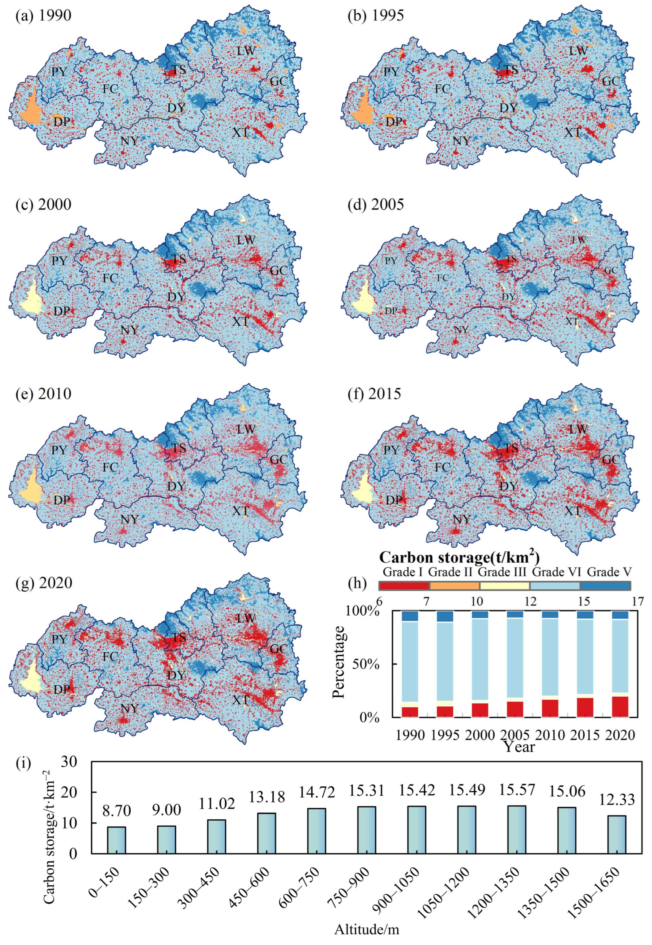
From 1990 to 2020, carbon storage in the study area exhibited a distinct spatiotemporal evolution. Spatially, the pattern underwent restructuring characterized by the expansion of low-value zones and the fragmentation of high-value zones (Figure 3). Temporally, it followed a trajectory of “initial increase, subsequent decline, and eventual stabilization.” The spatial distribution displayed observable shifts. High carbon storage zones were initially widespread, but over time, low-value zones (Grade I) expanded significantly, particularly in the northeastern and southeastern counties (TS, LW, and XT) (

Table 6. Carbon storage value (t/km²) in different counties from 1990 to 2020.

Year	DY	DP	FC	GC	LW	NY	PY	TS	XT
1990	9.55	8.52	8.84	9.68	9.90	8.71	9.20	10.01	8.95
1995	9.54	8.56	8.83	9.69	9.88	8.70	9.18	9.95	9.07
2000	9.91	8.94	9.26	9.73	9.93	9.06	9.40	10.25	9.28
2005	9.83	8.88	9.14	9.59	9.83	9.02	9.27	10.09	9.21
2010	9.80	8.86	9.15	9.50	9.81	8.99	9.31	10.01	9.18
2015	9.82	8.86	9.14	9.47	9.82	8.96	9.36	10.01	9.17
2020	9.69	8.84	9.12	9.52	9.82	8.94	9.43	9.81	9.18

). Meanwhile, DP County in the southwest remained a persistent lower-value region. During 1990–2000, carbon storage patterns optimized and reached their peak; TS County, for example, increased from 10.01 to 10.25 t/km². Between 2010 and 2020, patterns stabilized but showed localized degradation, marked by expanding low-value zones. By 2020, DP County’s carbon storage had declined to 8.84 t/km², a 1.1% drop from its 2000 peak.

Temporally, the total carbon storage fluctuated. Rapid growth from 1990 led to a peak around the year 2000 for most counties, followed by a declining trend that stabilized by 2020. Concurrently, the grade structure shifted noticeably: the proportion of low-grade zones (Grade I) expanded, rising from approximately 10% in 1990 to nearly 20% by 2020. Grade III consistently remained the dominant class throughout the study period, comprising most of the total area, while the proportion of high-grade zones (Grade V) remained relatively small and stable. At the county scale, despite the expansion of Grade I areas, TS and LW counties maintained consistently high average carbon storage (>9.80 t/km²), functioning as key regional carbon sinks, whereas DP County remained a region with relatively limited sequestration potential.

4.1.2. Spatiotemporal Dynamics of Water Yield

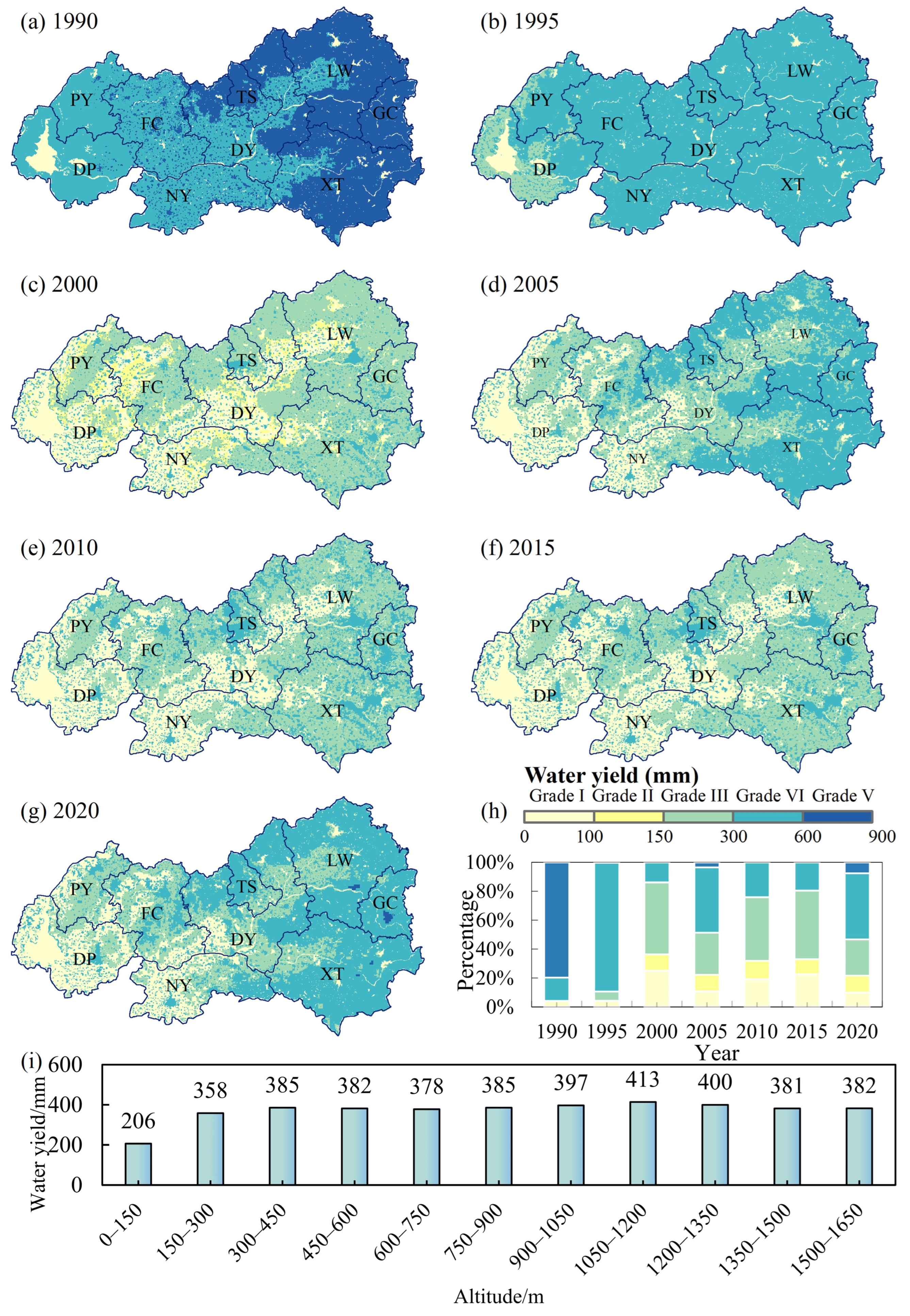
The spatiotemporal dynamics of water yield in the study area (1990–2020) differed significantly from carbon storage, exhibiting a much greater magnitude of fluctuation and a distinct evolutionary trajectory, ultimately forming an “east-to-west decreasing” spatial gradient. Spatially, the water yield pattern underwent dramatic volatility and overall contraction. High water yield zones (Grade V: 600–900 mm) were most extensive in 1990, overwhelmingly concentrated across GC, XT, and other eastern counties. From 1995 to 2000, this spatial pattern shrank drastically, and high-yield zones virtually disappeared. Most counties degraded to medium-low grades. Consequently, low-value zones (Grades I–II) dominated the study area, particularly in southwestern regions such as DP County. After 2000, a fluctuating recovery occurred but failed to revert to the 1990 level. By 2020, a clear east–west gradient with significant regional disparity was established, the water yield in DP County was merely 33.9% of that in GC County.

Temporally, the total water yield presented a “sharp initial decline followed by volatile fluctuation” pattern, in sharp contrast to the gradual trends observed in carbon storage (Figure 4). It declined sharply to a trough between 1990 and 2000, remaining significantly lower than the 1990 baseline by 2020. The grade structure changed markedly, characterized by a dramatic loss of high-yield areas and dominant fluctuations in medium grades. Specifically, Grade V plummeted after 1990, while the proportion of Grade I spiked around 2000 and continued to fluctuate. Post-2000, medium-yield zones (Grades III and IV) alternately dominated the landscape. Significant county-level heterogeneity was observed: GC and TS counties consistently maintained annual average water yields above the regional mean, while DP County remained the lowest. Volatility varied greatly, with DY and GC counties experiencing the most intense fluctuations. Furthermore, water yield exhibited a clear topographical response, peaking at 413 mm within the 1050–1200 m elevation band before slightly plateauing at higher altitudes. The high-yield period (1990–1995) was primarily driven by abundant precipitation, while the general declining trend and subsequent fluctuations after 1995 were likely attributed to the combined effects of climate variability and land use change (

Table 7. Water yield value (mm) in different counties from 1990 to 2020.

Year	DY	DP	FC	GC	LW	NY	PY	TS	XT
1990	582.21	406.10	539.65	661.19	636.27	520.40	497.01	622.70	625.78
1995	384.88	269.49	362.66	430.67	411.64	345.90	338.10	412.68	412.95
2000	183.89	122.10	186.41	258.99	220.59	160.11	174.99	219.23	248.38
2005	274.21	137.33	234.62	355.35	311.82	224.59	194.44	323.97	353.06
2010	223.57	122.58	209.50	302.46	266.08	170.96	187.62	285.09	272.80
2015	212.17	125.33	203.34	267.70	234.73	172.90	185.70	269.74	256.84
2020	290.75	142.17	243.64	419.46	360.24	226.04	212.78	358.41	379.56

).

4.2. Spatiotemporal Distribution Pattern of Carbon–Water Coupling Degree

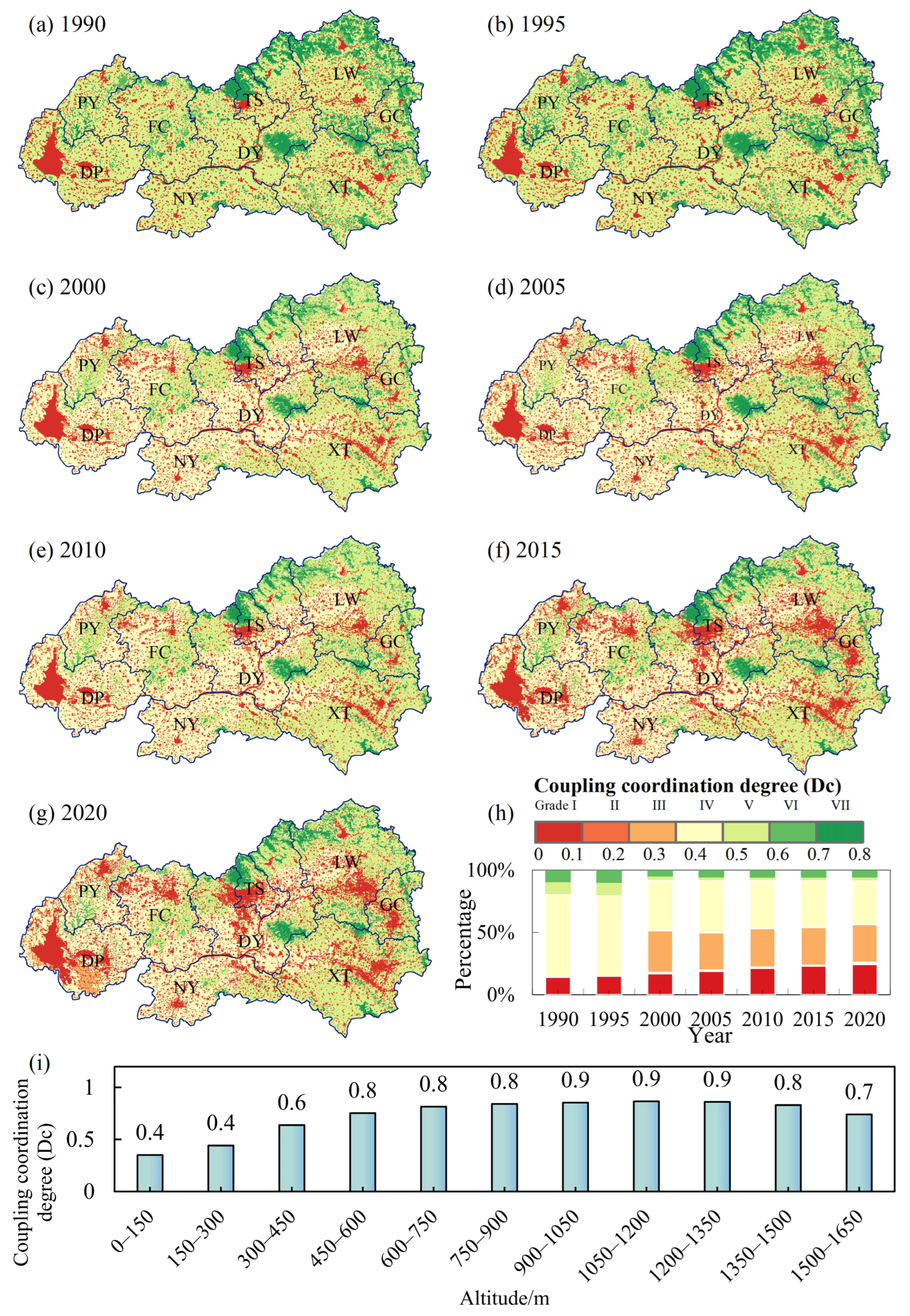
The spatiotemporal dynamics of the coupling coordination degree (CCD) between carbon storage and water yield from 1990 to 2020 exhibited a clear trend of overall degradation and spatial fragmentation (Figure 5). Spatially, the pattern was characterized by the continuous expansion of severely uncoordinated zones (Grade I, red areas) and the shrinking of relatively coordinated zones (Grades V and above). In 1990 and 1995, the study area was widely dominated by medium-to-high coordination. However, by 2020, low-value zones (Grade I) had visibly expanded and aggregated, particularly radiating across DP, TS, LW, and XT counties. DP County in the southwest consistently remained the primary low-value center throughout the study period.

Temporally, the average CCD across the region experienced a trajectory of “initial stability, abrupt decline, and subsequent low-level stagnation” (

Table 8. CCD value in different counties from 1990 to 2020.

Year	DY	DP	FC	GC	LW	NY	PY	TS	XT
1990	0.45	0.33	0.41	0.46	0.47	0.39	0.42	0.44	0.42
1995	0.45	0.33	0.41	0.46	0.47	0.39	0.42	0.43	0.43
2000	0.36	0.27	0.34	0.40	0.39	0.31	0.34	0.35	0.37
2005	0.37	0.25	0.33	0.39	0.39	0.32	0.33	0.34	0.37
2010	0.36	0.24	0.33	0.37	0.38	0.30	0.33	0.33	0.35
2015	0.35	0.24	0.32	0.35	0.36	0.30	0.33	0.31	0.35
2020	0.34	0.22	0.30	0.36	0.37	0.29	0.31	0.30	0.35

). Between 1990 and 1995, county-level CCDs were at their highest and remained stable, led by LW (0.47) and GC (0.46) counties. A dramatic region-wide drop occurred in 2000, followed by a gradual downward trend until 2020. By the end of the study period, DP County recorded the lowest CCD of 0.22 (a 33.3% drop from its 1990 level), while LW and GC counties maintained the highest relative values (0.37 and 0.36, respectively), though still significantly degraded from their historical peaks.

The structural composition of CCD grades firmly corroborated this degradation process (Figure 5h). In the early 1990s, Grade IV was the absolute dominant class. Post-2000, this structure collapsed: the proportion of Grade IV shrank drastically, while lower coordination grades (Grades I and III) expanded substantially. Notably, the proportion of Grade I steadily increased from approximately 10% in 1990 to over 20% by 2020, underscoring an intensifying spatial conflict between carbon sequestration and water yield services.

Furthermore, the CCD demonstrated a highly sensitive response to topographical gradients (Figure 5i). The coordination degree increased significantly with elevation, rising from a low of 0.4 in plain areas (0–150 m) to a stable peak of 0.9 within the mid-to-high altitude band (900–1350 m), before experiencing a slight decline at extreme elevations (>1500 m). This highlights that higher-altitude forested or mountainous regions serve as the core ecological buffers maintaining carbon–water synergy.

4.3. Trends of the Carbon–Water Coupling Coordination Degree

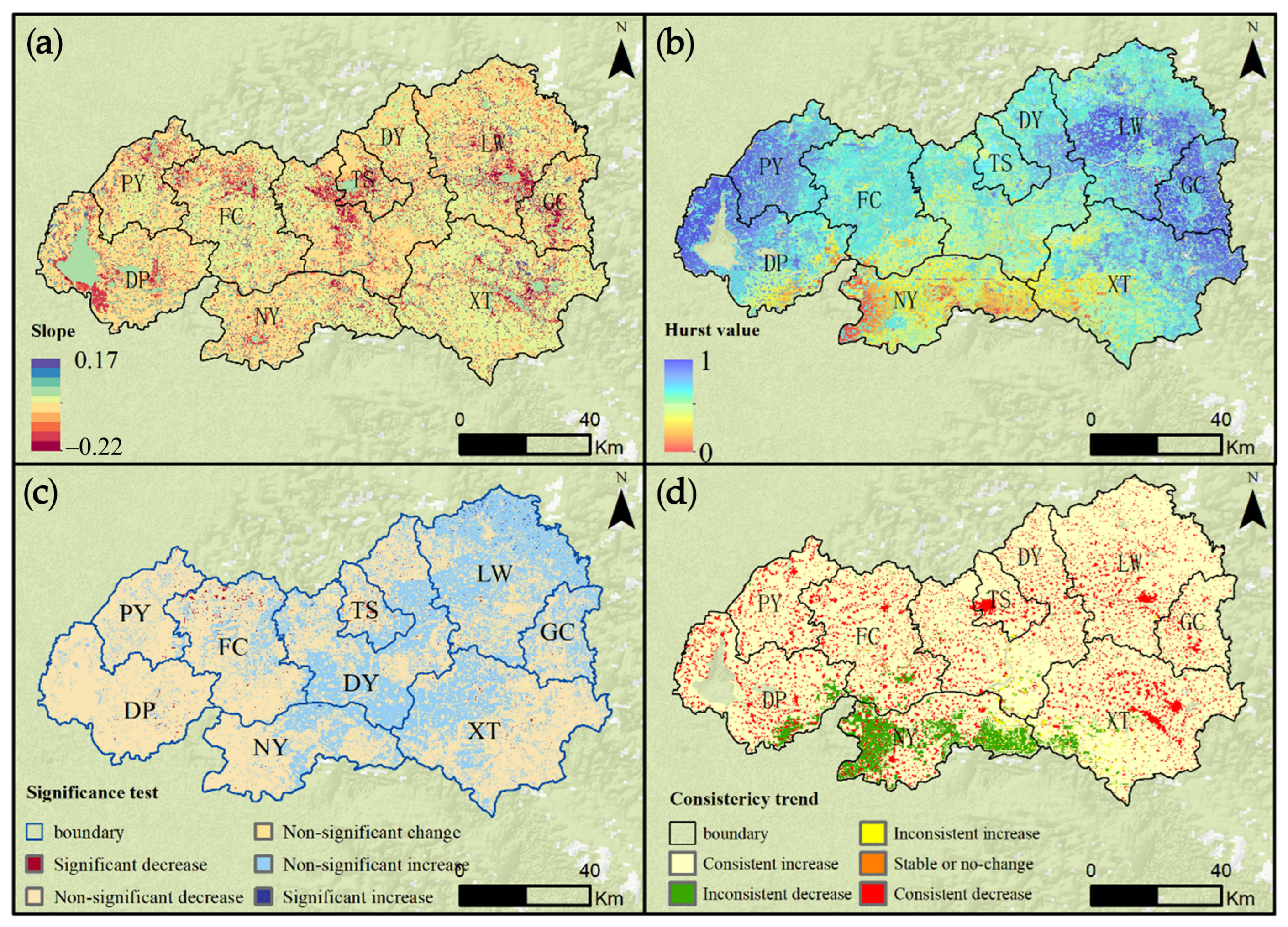
From a spatial distribution perspective, the slopes varied significantly across regions, ranging from −0.22 to 0.17 (Figure 6). Overall, negative slopes were observed in multiple regions, indicating a dominant downward trend in the time series of the indicator within the study area. The Hurst values ranged from 0 to 1, reflecting different persistence characteristics across regions. Some regions exhibited higher Hurst values, indicating stronger persistence, while others showed lower Hurst values and weaker persistence. Overall, the persistence pattern of the indicator in the study area was complex, with clear regional differences in the future trend persistence.

Significance testing categorized regions into types such as non-significant change, significant decrease, non-significant increase, and significant increase. Spatially, non-significant change areas were widely distributed, while significant change areas were relatively scattered. Areas of significant decrease and significant increase were sporadically distributed, indicating that the statistical significance of changes in the indicator exhibited a dispersed spatial pattern, with clear regional differences in significance. Different trend types were interwoven spatially, with consistent decrease areas showing certain spatial clustering. This suggests that the trend consistency pattern of the indicator in the study area was complex, with clear regional differences in consistency. Overall, the carbon sink-water yield coupling coordination degree in the Dongping Lake Basin exhibited a dominant improving trend. Specifically, areas of significant increase were concentrated in the central and northern regions, such as the DY area, while areas of significant decrease were sporadically distributed in the central and southern regions, such as the western part of the NY area and the eastern part of the DY area.

4.4. Driving Factors of Changes in Carbon–Water Coupling Relationships

The influence of 12 driving factors on the spatial heterogeneity of the coupling coordination degree (CCD), alongside their temporal evolution from 1990 to 2020, was systematically analyzed using both spatial factor detection (q-values) and global feature importance evaluation (

Table 9. Results of carbon–water coupling coordination relationships factor detection (q-value).

Driving Factors	1990	1995	2000	2005	2010	2015	2020
Precipitation (X1)	0.16	0.18	0.08	0.14	0.21	0.12	0.14
Temperature (X2)	0.33	0.31	0.37	0.39	0.36	0.34	0.38
Slope (X3)	0.41	0.41	0.54	0.49	0.52	0.51	0.5
Elevation (X4)	0.36	0.35	0.44	0.44	0.43	0.4	0.43
NDVI (X5)	0.23	0.29	0.15	0.21	0.22	0.25	0.29
Soil sand content (X6)	0.02	0.01	0.02	0.02	0.02	0.01	0.02
Soil silt content (X7)	0.06	0.05	0.06	0.06	0.06	0.05	0.06
Soil clay content (X8)	0.01	0.01	0.03	0.02	0.03	0.03	0.03
Population (X9)	0.12	0.16	0.15	0.15	0.12	0.07	0.11
GDP (X10)	0.11	0.15	0.14	0.11	0.11	0.06	0.08
DMSP (X11)	0.09	0.13	0.13	0.14	0.23	0.23	0.2
Land use type (X12)	0.59	0.6	0.5	0.5	0.5	0.5	0.49

).

The results reveal a dual-driven mechanism shaped by categorical spatial controls and continuous topographic-environmental variables. According to the spatial factor detection (Table 9), land use type (X12) consistently exhibited the highest q-values across all seven periods (0.49–0.60), followed by slope (X3, 0.41–0.54), elevation (X4, 0.35–0.44), and temperature (X2, 0.31–0.39). This indicates that land use patterns, together with topographic factors, jointly constitute the fundamental spatial framework controlling the distribution of the CCD. Notably, the explanatory power of land use declined modestly from 0.59–0.60 in the 1990s to 0.49–0.50 after 2000, suggesting a gradual shift toward more diversified spatial controls. Meanwhile, socio-economic factors such as DMSP nighttime light (X11) demonstrated an increasing trend (from 0.09 in 1990 to 0.20 in 2020), reflecting the growing role of urbanization in reshaping the spatial heterogeneity of the CCD. 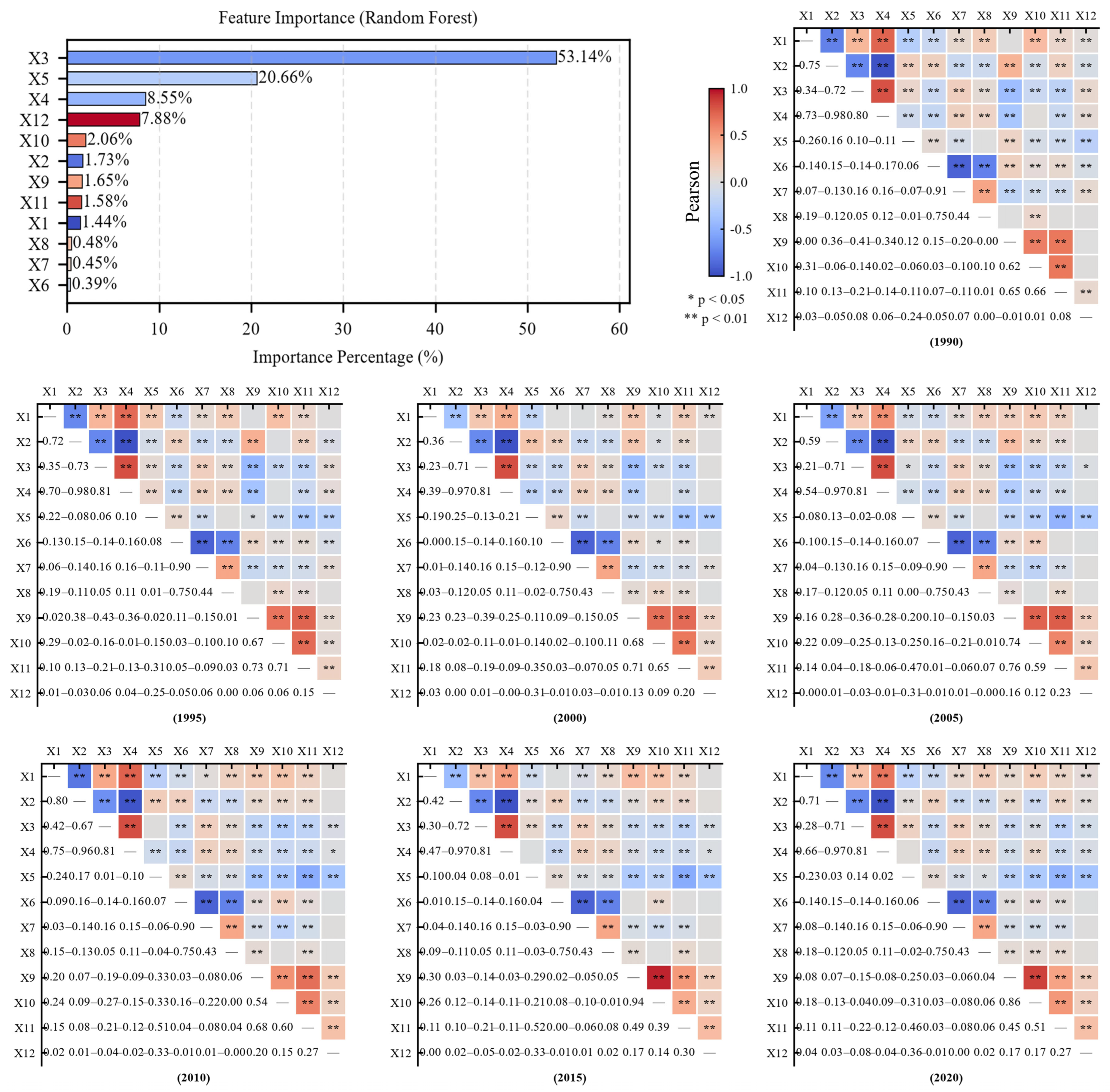From a global feature importance perspective (Figure 7), continuous topographic and environmental variables exerted the most substantial overall influence, with slope (X3, 10.10%), NDVI (X5, 10.09%), and precipitation (X1, 10.08%) emerging as the top three contributing features. The integration of these results suggests that while land use type and topography dictate the macro-spatial framework, local variations are fine-tuned by hydrothermal conditions and biophysical gradients.

Temporally, dynamic factors exhibited distinct evolutionary trajectories. NDVI (X5) displayed a pronounced V-shaped pattern, declining from 0.23 (1990) to a historical low of 0.15 in 2000, before recovering steadily to 0.29 by 2020. This trajectory likely reflects the initial disruption of natural vegetation cover during the aggressive agricultural expansion of the 1990s, followed by progressive ecological recovery driven by large-scale reforestation and ecological restoration projects implemented after 2000. DMSP nighttime light (X11) exhibited a substantially strengthened influence, with its q-value nearly tripling from 0.09 (1990) to a plateau of 0.23 (2010–2015), before moderating slightly to 0.20 in 2020—underscoring the intensifying role of urbanization in reshaping the CCD’s spatial heterogeneity, with the post-2015 moderation potentially signaling a transition toward more spatially balanced development patterns. In contrast, socio-economic factors exhibited unsynchronized but converging declining trajectories. Population density (X9) and GDP (X10) both peaked early—at 0.16 and 0.15, respectively, around 1995—before declining to lows of 0.07 and 0.06 by 2015. This early peak followed by sustained decline suggests that the mid-1990s represented a period when spatially concentrated demographic and economic expansion most strongly conditioned the CCD; in subsequent decades, the dilution of these direct spatial effects may reflect a regional shift from concentrated scale-driven development toward more diffuse, quality-oriented socio-economic transformation. Precipitation (X1), by contrast, displayed notable inter-decadal variability (q = 0.08–0.21), with distinct peaks in 1995 (0.18) and 2010 (0.21), indicating that the explanatory power of climatic factors responds to multi-year hydroclimatic cycles rather than monotonic long-term trends.

Furthermore, multi-period Pearson correlation heatmaps and Random Forest importance ranking (Figure 7) revealed a hierarchically coupled driving structure. Slope (X3) and NDVI (X5) were the predominant drivers, contributing 53.14% and 20.66% of total importance, respectively, followed by elevation (X4, 8.55%) and land use (X12, 7.88%). Socioeconomic variables—GDP, population, and nighttime lights—each accounted for less than 2.1%, indicating limited direct explanatory power. Correlation patterns remained temporally stable across 1990–2020: elevation was strongly negatively correlated with temperature (r = −0.75 to −0.98, p < 0.01) and positively correlated with slope (r = 0.70–0.98, p < 0.01), while significant collinearity persisted among soil textural components. Interlinkages among socioeconomic factors intensified from r = 0.54–0.68 in 1990 to r = 0.76–0.94 by 2020 (p < 0.01). These results underscore that CCD dynamics are governed not by additive individual effects but by a deeply interwoven natural–social system, wherein physiographic factors serve as primary controls and anthropogenic drivers operate predominantly through synergistic interactions.

5. Discussion

5.1. Carbon–Water Coordination Relationship

This study reveals a significant spatiotemporal mismatch between carbon storage and water yield in the Dongping Lake Basin (DLB). Although carbon storage exhibited an overall trend of “initial increase followed by stabilization,” water yield experienced drastic fluctuations and an overall decline. The mean Coupling Coordination Degree (CCD) between these two services was merely 0.23, indicating a low level of coordination [38,39]. This finding not only confirms the widespread ecosystem service trade-off effect in the Yellow River Basin [40,41], but also strongly aligns with recent international observations in semi-arid and Mediterranean basins globally [11]. In these transitional climatic zones worldwide, ecological restoration often presents a double-edged sword. While vegetation recovery significantly enhances carbon storage capacity through photosynthesis, it is concurrently accompanied by increased canopy interception and elevated evapotranspiration rates [42]. This process substantially increases soil water consumption, partially or fully offsetting potential increases in water yield [43,44,45]. It becomes evident that the spatial mismatch and low coordination degree observed here are not isolated local phenomena, but rather a prevalent ecological threshold challenge shared by semi-humid to semi-arid transitional watersheds globally. Notably, during the 1990–2000 period in the DLB, a sharp decline in water yield stood in stark contrast to the concurrent optimization of the carbon storage pattern. This suggests that high-intensity land-use changes in the early stage may have disrupted the pre-existing hydrological balance. Therefore, whether in the Mediterranean region or the DLB, solely pursuing the enhancement of carbon sinks while neglecting the regional water resource carrying capacity could inadvertently exacerbate water scarcity risks. This underscores the global urgency of seeking a sustainable “carbon–water” win–win balance in watershed ecological management.

5.2. Multi-Factor Interactions and Dominant Driving Mechanisms

While single-factor detection identifies land-use type (X12) as the dominant driver of spatial heterogeneity in CCD (q > 0.7049), it is not the sole explanatory mechanism. To elucidate the physical mechanisms underlying this statistical dominance—and specifically to explain the severe carbon–water decoupling observed during the 1990s—a detailed analysis of land-use transition matrices was conducted (Figure 8). As visualized in the chord diagrams, the 1990–2000 period experienced a dramatic cascade of land-cover restructuring. Intensive agricultural reclamation and early-stage urbanization fundamentally severed pre-existing eco-hydrological continuums. For instance, between 1995 and 2000, agricultural expansion aggressively encroached upon ecological spaces, resulting in the direct conversion of 578.68 km² of grassland, 317.63 km² of forest land, and 113.70 km² of water bodies into cropland. Concurrently, rapid urbanization consumed massive tracts of agricultural land, with 475.30 km² of cropland transitioning into built-up land. This intense fragmentation of continuous ecological patches physically disrupted natural surface runoff and evapotranspiration processes, providing direct mechanistic evidence for the drastic decline in regional water yield and the sharp drop in the CCD during this specific historical phase.

Furthermore, a pivotal finding of this study is that although temperature (X2) has weak individual explanatory power, its interaction with elevation (X4) exhibits the strongest combined effect. This reveals a non-linear modulation mechanism where the natural substrate conditions regulate climatic drivers: under identical temperature conditions, elevation dictates vegetation growth efficiency and runoff processes by modulating the thermal growing season length and orographic precipitation redistribution, thereby reshaping the spatial patterns of carbon–water coupling [46]. This suggests that ecosystem services in the DLB are not driven unilaterally by anthropogenic activities but are the result of a complex “climate–soil–human activity” coupling system. Land-use changes, such as urban expansion and agricultural reclamation, directly sever or restructure the original carbon–water cycles, while topographic and pedological conditions constitute the physical boundary constraints for these transformations [40].

A detailed analysis of land-use transition matrices, visualized via chord diagrams (Figure 8), reveals that the severe carbon–water decoupling observed between 1990 and 2000 was driven by a dramatic and rapid cascade of land-cover restructuring. This decade witnessed intense agricultural reclamation and early-stage urbanization that fundamentally altered the basin’s hydrological and ecological balance. Specifically, during the 1995–2000 period, agricultural expansion aggressively encroached upon critical ecological spaces, resulting in the conversion of 578.68 km² of grassland, 317.63 km² of forest land, and 113.70 km² of water bodies into cropland. Concurrently, rapid urbanization consumed massive tracts of agricultural land, with 475.30 km² of cropland transitioning directly into built-up land. This intense fragmentation of continuous ecological patches severely disrupted natural surface runoff and evapotranspiration processes, directly explaining the drastic decline in regional water yield and the sharp drop in the explanatory power of static land-use patterns during this specific historical phase.

It is also noteworthy that individual soil properties (X6, X7, X8) consistently yielded relatively low q-values (0.01–0.06) and contributed marginally to spatial differentiation in the single-factor analysis. This phenomenon occurs fundamentally because soil texture acts as a highly stable, static macro-background variable, exhibiting negligible spatiotemporal variation over a 30-year period at a 1-km resolution. Consequently, as independent drivers of dynamic change, their statistical signal appears weak. However, their critical ecological role is unveiled through multi-factor interactions: soil properties function as the indispensable physical matrix that heavily dictates infiltration and water-holding capacities. They synergistically amplify or buffer the impacts of dynamic variables, which perfectly explains why the interaction between precipitation and soil sand content demonstrated the strongest overall spatial explanatory power despite the low individual determinant power of soil factors.

5.3. Hierarchical Management Strategies Under Spatiotemporal Heterogeneity

The results demonstrate a pronounced elevation-dependency of the CCD, with degradation primarily concentrated in the northwestern regions. Based on these spatiotemporal heterogeneities, we propose differentiated ecological management strategies based on altitudinal gradients [47,48]. For high-altitude areas (>1000 m) in the southeast and central mountains, the high CCD suggests a relatively balanced vegetation-hydrology relationship [49]. These areas should be designated as Core Ecological Protection Zones, adopting a strategy centered on “natural restoration supplemented by minimal intervention” to maintain the stability of water yield and carbon pool functions. Conversely, the northwestern low-altitude agricultural plains, characterized by high human intensity and declining coupling trends, should be prioritized as Ecological Restoration Zones. We recommend promoting water-saving eco-agriculture and optimizing crop structures to reduce unproductive evaporation. Furthermore, in the process of urbanization, the uncontrolled expansion of impervious surfaces must be strictly regulated. Implementing green infrastructure, such as rain gardens and ecological corridors, could mitigate the loss of water yield and carbon sequestration caused by surface hardening, thereby alleviating the conflict between human development and land preservation. thereby alleviating the conflict between human development and land preservation. Furthermore, the direct integration of these quantitative ecosystem service metrics into statutory land-use planning frameworks is highly recommended to bridge the gap between ecological assessments and operational territorial management. Based on the spatial divergence of the CCD, management strategies must be tailored to specific local conditions. In the High-Altitude Source Zones (primarily in the east and northeast), ecological management should shift from aggressive, high-density afforestation to “natural restoration supplemented by minimal intervention.” To balance the carbon–water trade-off, forestry planning must strictly prioritize native, low-water-consuming broadleaf species or mixed forests over high-transpiration exotic coniferous species, ensuring that carbon sink enhancement does not deplete critical headwater yields.

Conversely, the Low-Altitude Agricultural Plains and Riparian Zones (primarily in the west and southwest) require urgent, concrete interventions to mitigate severe carbon–water decoupling. First, in agricultural zones, generalized “water-saving” appeals must be translated into the enforcement of precision drip-irrigation networks and the substitution of water-intensive crops with drought-resistant rotations. Second, within the immediate lake buffer zones, strict ecological environment survey standards for lakes and wetlands should be implemented. Management here should focus on constructing engineered wetlands and restoring native emergent and submerged aquatic vegetation. This approach maximizes localized carbon sequestration and intercepts non-point source agricultural runoff, acting as a critical buffer to stabilize the regional carbon–water coordination under intensifying human activities.

5.4. Limitations and Future Perspectives

Despite revealing the evolutionary patterns of carbon–water coupling in the DLB at a macro scale, this study has limitations. First, the InVEST model relies on simplified hydrological assumptions; while effective at an annual scale, it overlooks groundwater interactions and the instantaneous impacts of seasonal extreme climate events, which may introduce biases in water yield estimation [50,51]. Second, a notable methodological limitation arises from the spatial heterogeneity of the input datasets. While land-use and topographic (DEM) data were obtained at a fine 30-m resolution, meteorological and soil datasets were available only at a 1-km resolution. Resampling these coarser grids to match the 30-m scale introduces inherent uncertainty. Specifically, in the topographically heterogeneous transition zones of the basin, 1-km climate data effectively smooths out critical micro-climatic variations, such as localized temperature gradients and small-scale orographic precipitation differences. This resolution disparity might obscure fine-scale coupling patterns between carbon and water cycles, leading to potential underestimations of ecological trade-offs in highly variable terrain. To overcome this in future research, we should integrate high-frequency data from Eddy Covariance (flux tower) observations for localized parameter calibration and incorporate higher-resolution remote sensing products.

Furthermore, while most studies adopt equal weighting (α = β = 0.5) based on the premise that subsystems contribute equally to overall coordination, an emerging body of literature has tested this assumption through sensitivity analyses. For instance, study on cultural–tourism industry coupling in port cities conducted a systematic sensitivity analysis with varying weight allocations (α = 0.7, β = 0.3 for heritage-rich cities; α = 0.3, β = 0.7 for service economies; and α = 0.5, β = 0.5 as the baseline), demonstrating that coordination rankings remained highly stable with Spearman correlation coefficients exceeding 0.91 across all scenarios, although absolute coordination values varied by ±0.08–0.15 units depending on weight selection [52]. Similarly, research on the Chengdu–Chongqing urban agglomeration employed the CCD model with equal weights for social economy and ecological environment subsystems, acknowledging that the equal-weighting assumption represents a neutral baseline for cross-regional comparison while noting that context-specific adjustments may be warranted for city-specific policy assessments [53]. In the context of the Dongping Lake Basin, where water security is paramount for agricultural productivity and regional ecological stability, the equal and static weighting adopted herein—while justified by the basin’s dual strategic mandates as a water regulation node for the South-to-North Water Diversion Project and a national carbon sink under China’s “Dual Carbon” framework—may obscure localized vulnerabilities in sub-watersheds facing severe agricultural water demands or seasonal hydrological droughts. Future research should thus incorporate dynamic weighting scenarios (e.g., assigning higher weight to water yield during dry years or in heavily irrigated zones, potentially via AHP–entropy hybrid methods) to better capture trade-offs dictated by localized ecological and socioeconomic pressures [54,55]. Ultimately, advancing this dynamic approach requires developing actionable pathways to explicitly incorporate carbon–water coupling results into operational territorial planning frameworks based on ecosystem services [56].

6. Conclusions

This study advances the current state of watershed ecological research by shifting the analytical paradigm from isolated, static ecosystem service assessments to a dynamic, long-term interactive framework. By quantifying the spatiotemporal continuum of carbon–water coupling in a highly pressured transitional basin over 30 years, this research uncovers the non-linear driving mechanisms among anthropogenic land-use boundaries and natural climate–––soil substrates. The primary theoretical and empirical contributions are summarized as follows:

(1)

Fundamental Spatial Mismatch and Trade-off Dynamics: Carbon storage and water yield exhibit profound spatiotemporal divergence, confirming a persistent trade-off effect characteristic of transitional watersheds. While carbon storage demonstrated a relatively stable “rise-then-plateau” trajectory, water yield suffered severe fluctuations and long-term decline. The resulting spatial mismatch—characterized by robust coordination in high-altitude eastern zones versus severe decoupling in the human-dominated southwestern plains—underscores the critical risk of pursuing carbon sink enhancement at the expense of regional water carrying capacity.

(2)

Trajectory of Coupling Degradation and Altitudinal Dependency: The overall coupling coordination between the two services remains at a concerningly low level. Temporally, the system experienced a trajectory of “initial stability, abrupt decline post-2000, and subsequent low-level stagnation.” Spatially, the coupling relationship exhibits a strict altitudinal dependency, where mid-to-high alpine zones function as indispensable ecological buffers, while lower-elevation agricultural and urban interfaces face continuous degradation and severe spatial fragmentation.

(3)

Hierarchical “Human–Natural” Driving Mechanisms: The spatial heterogeneity of carbon–water coupling is not driven by isolated factors, but by a hierarchically interwoven natural–social system. Intense anthropogenic land-use changes—specifically the conversion of ecological lands to agriculture and built-up areas—act as the absolute dominant spatial determinant, effectively dictating the macro-framework of the coupling relationship. Simultaneously, static physiographic factors (topography and soil texture) function as essential physical constraints that non-linearly amplify or buffer the highly dynamic, localized impacts of climatic fluctuations.

Ultimately, these findings underscore the need to transition from uniform management models toward spatially explicit, adaptive ecological governance. Future ecological restoration must abandon generalized approaches in favor of targeted, spatially explicit interventions—prioritizing minimal intervention in high-altitude source zones and stringent, water-saving eco-agricultural infrastructure in the decoupled lowland plains.