Asynchronous Evolution of Urbanisation and the Ecological Environment in Southeast Asia

Abstract

Accelerated urbanisation and associated land-use conversion are reshaping the composition and functions of terrestrial ecosystems globally. In Southeast Asia, ecological change is increasingly mediated not only by demographic urbanisation but also by urban expansion, peri-urban development, and the conversion of agricultural, coastal, and forest land into built-up surfaces. This study integrates multi-source geographical information from 2014 to 2024 to examine 351 provincial-level units in 11 Southeast Asian nations. To describe the spatial-material dimension of urbanisation and ecological conditions, two indices were created: the Composite Nighttime Light Index (CNLI), used as a proxy for urban expansion and built-up development intensity, and the Improved Remote Sensing Ecological Index (IRSEI), which is tailored to tropical coastal locations. The development of human-environment interactions was measured using the Coupling Coordination Degree (CCD) model. Pathways of synergy and trade-off were found using an incremental four-quadrant framework, and nonlinear causes of spatial differentiation were investigated using Spearman correlation and the Optimal Parameter-based Geographical Detector (OPGD). Uncertainty was addressed through data-quality masking, annual compositing, consistent index-construction rules, and cautious interpretation of CCD and driver results as relative provincial-scale patterns. The regional mean CCD rose from 0.250 to 0.314 during the decade, showing a slow improvement; nevertheless, most places still have low to moderate levels of coordination. There is clear pathway divergence, with 38.7% of locations enduring trade-offs where built-up development happens at the price of ecological quality and 58.4% of regions seeing synergistic improvement. The coupling pattern is primarily driven by built-up area expansion, with multiple factors jointly producing strong nonlinear enhancement effects. Climate conditions and forest disturbance further strengthen these effects. This study extends beyond single-country analyses by situating remote-sensing coupling results within land-use transition, peri-urbanisation, urban–rural linkage, and regional-governance perspectives. It provides quantitative evidence to support differentiated policy strategies in rapidly urbanising places.

1. Introduction

Global urbanisation is affecting the functioning and configuration of natural ecosystems [1]. However, urbanisation should not be understood only as population growth or an increase in the share of urban residents. It is also a territorial and land-use transition through which agricultural land, wetlands, forests, coastal zones, and peri-urban villages are converted into built-up land, infrastructure corridors, industrial estates, and suburban settlements [1,2,3,4]. This distinction is important because the ecological consequences of urban growth are transmitted mainly through land conversion, landscape fragmentation, soil sealing, heat accumulation, hydrological alteration, and the displacement of ecological pressures across urban–rural systems [3,5,6,7]. Therefore, in this paper, “urbanisation” is used as an umbrella concept, while “urban expansion”, “built-up development”, and “land-use conversion” are used when the discussion refers specifically to the spatial-material processes captured by nighttime-light and built-up-area indicators.

These processes are particularly important in Southeast Asia. The region has experienced rapid growth of metropolitan regions, secondary cities, port-industrial corridors, tourism-oriented coastal development, and peri-urban settlement belts, many of which blur the conventional boundary between urban and rural space [4,8,9,10,11]. According to the United Nations World Urbanisation Prospects, the proportion of people in this region who live in cities grew from 38% in 2000 to 51% in 2020 and is expected to reach 66% by 2050 [12]. Yet the ecological impacts of this transition depend less on population shares alone than on where new built-up surfaces emerge, which land uses they replace, and how regional governance manages urban–rural flows of labour, food, energy, water, construction materials, and ecological services [3,7]. Large-scale land conversion [9], more extreme thermal conditions [13], and forest loss [14] are all consequences of rapid population growth and geographic expansion. Southeast Asia’s annual deforestation rate is among the highest in the world, with a cumulative loss of over 60 million hectares of forest cover between 2001 and 2023 [15]. Structural conflicts frequently worsen because regional environmental governance systems are often unable to keep pace with the speed and spatial complexity of built-up development. For the region’s transition to sustainability, it is crucial to investigate how coordinated environmental improvements can be achieved during this time of rapid urban expansion.

Accurate measurement is required for regional collaborative governance, and complex system dynamics can be quantified by deeply integrating multi-source spatial data into cloud computing platforms. Unlike traditional statistical data, which are constrained by administrative boundaries and spatial discontinuities, nighttime light (NTL) remote sensing data directly reflects the intensity of human growth by capturing surface light radiation. Researchers have developed a high-dimensional analytical framework for error correction, algorithmic calibration, and multi-scenario applications, including pixel-level light correction and cross-border urban growth dynamics [16]. Using cloud computing, the Remote Sensing Ecological Index (RSEI) establishes a fundamental framework for quantitative ecological assessment by combining natural factors without subjectivity. Its applications have expanded to include long-term high-frequency tracking of ecological evolution [17,18], reconstruction of continuous frameworks to address algorithmic instability [19,20], localised modelling for complex land surface conditions [21], and deconstruction of spatial heterogeneity using multi-source drivers [22,23]. It has also taken significant steps toward new interdisciplinary perspectives, including sustainable empowerment via digital infrastructure [24], multidimensional evaluation of circular cities [25], and resilient collaborative development in coastal cities [26]. After quantifying individual system elements, the coupling coordination framework provides a useful approach for analysing cross-system interactions. Numerous studies have applied the Coupling Coordination Degree (CCD) model to characterise these relationships, resulting in a two-dimensional analytical framework of considerable breadth and depth—encompassing topics such as the feedback between urbanisation and the comprehensive ecological environment in core areas [27], trade-offs between urban expansion and ecosystem services [28], the impact of high-density development on ecological security baselines [29], the response of regional atmospheric environments to industrial agglomeration [30], the pressure on water environment carrying capacity from watershed urbanisation [31], exploration of the dual mechanisms of local spatial coupling and long-distance telecoupling [32], and the identification of spatiotemporal dynamics in specific ecologically fragile areas [33]. According to a review of the existing literature, such multi-dimensional coupling research is still primarily focused on macro-level coordination within individual countries or on mature mega-urban agglomerations such as the Beijing–Tianjin–Hebei region, the Shandong Peninsula, and the Chengdu–Chongqing region [34,35,36], as well as local provincial administrative units [37]. Related studies on eco-efficiency and carbon emissions efficiency further show that the sustainability effects of urbanisation can be nonlinear and stage-dependent, supporting the need to distinguish urban expansion from ecological outcomes [38,39].

Recent state-of-the-art research on urbanisation processes has moved beyond simple measurements of urban size to examine the mechanisms and morphologies of land development, including compact infill, edge expansion, leapfrog development, suburbanisation, peri-urbanisation, and telecoupled land change [1,3,10,40]. This process-oriented perspective is especially relevant for Southeast Asia because administrative units often contain mixed urban–rural landscapes: provincial cores, peri-urban townships, plantations, rice-growing areas, forest margins, and coastal settlements may coexist within the same unit. Consequently, the relationship between urban growth and ecological quality cannot be interpreted solely as a city-versus-nature contrast. It must be evaluated as a coupled land-use transition in which built-up development, rural restructuring, agricultural conversion, forest disturbance, and governance capacity jointly shape ecological outcomes.

However, several conceptual and methodological concerns remain when applying the coupling structure and assessment tools described above to Southeast Asia. (1) Assessment indicators have limited geographical applicability and conceptual scope. Traditional remote sensing ecological indices are vulnerable to regional inadaptability under tropical monsoon conditions and long, meandering coastlines, such as snow and ice indicator failure and vegetation index saturation. Meanwhile, a single nighttime-light intensity indicator struggles to fully capture the complex internal structure of urban sprawl, peri-urban development, and mixed urban–rural land-use conversion in developing countries. (2) Scenarios for transnational evolutionary pathways have yet to be identified. Current research frequently focuses on aggregate metrics within a single country, with limited empirical evidence on whether urban expansion produces synergistic ecological improvement, trade-off development, ecological recovery, or joint decline across regions with different land-use histories and governance capacities. (3) The nonlinear dynamics of driving processes have not been fully investigated. Previous research has primarily relied on traditional linear regression models, making it difficult to identify the deep-seated operational logic of nonlinear synergies and interaction amplifications caused by built-up expansion, population concentration, terrain constraints, climate conditions, and forest disturbances. (4) Uncertainty is rarely made explicit in coupling studies, even though remote-sensing preprocessing, cloud and water masking, index normalisation, PCA loading direction, spatial aggregation, and model-parameter choices may all affect the interpretation of CNLI, IRSEI, and CCD results.

Guided by these gaps, this study is organised around three research questions rather than only around a methodological workflow: (1) How have the spatial-material dimension of urbanisation and ecological environmental quality evolved across first-level administrative units in Southeast Asia during 2014–2024? (2) Which regions show synergistic improvement, trade-off development, ecological recovery, or joint decline, and how do these trajectories reveal peri-urban and land-use transition dynamics? (3) How do built-up development, population concentration, topography, forest disturbance, and climate factors interact to shape spatial differences in CCD? This study makes three main contributions. First, CNLI was developed for indicator system reconstruction by combining the average nighttime light intensity and the percentage of lighted pixels, but it is interpreted specifically as a proxy for urban expansion and built-up development intensity. Furthermore, localised factors such as the Bare Soil Index (SI) were combined to create an Improved Remote Sensing Ecological Index (IRSEI) tailored to tropical coastal environments, allowing for a more refined evaluation framework at the regional level. Second, this study moves beyond single-country analyses to identify transnational development pathways. Long-term transnational evolutionary patterns were quantitatively analysed using the Coupling Coordination Degree (CCD) model, and a refined four-quadrant framework was used to outline different development trajectories, including synergistic enhancement and trade-off limitations. Third, when examining driving mechanisms, conventional linear assumptions were rejected, and the Optimal Parameter-based Geographical Detector (OPGD) was used to identify dominant variables and nonlinear interactions. The interpretation further situates these quantitative results within theories of land-use transition, peri-urbanisation, urban–rural linkage, and regional governance.

2. Materials and Methods

2.1. Study Area

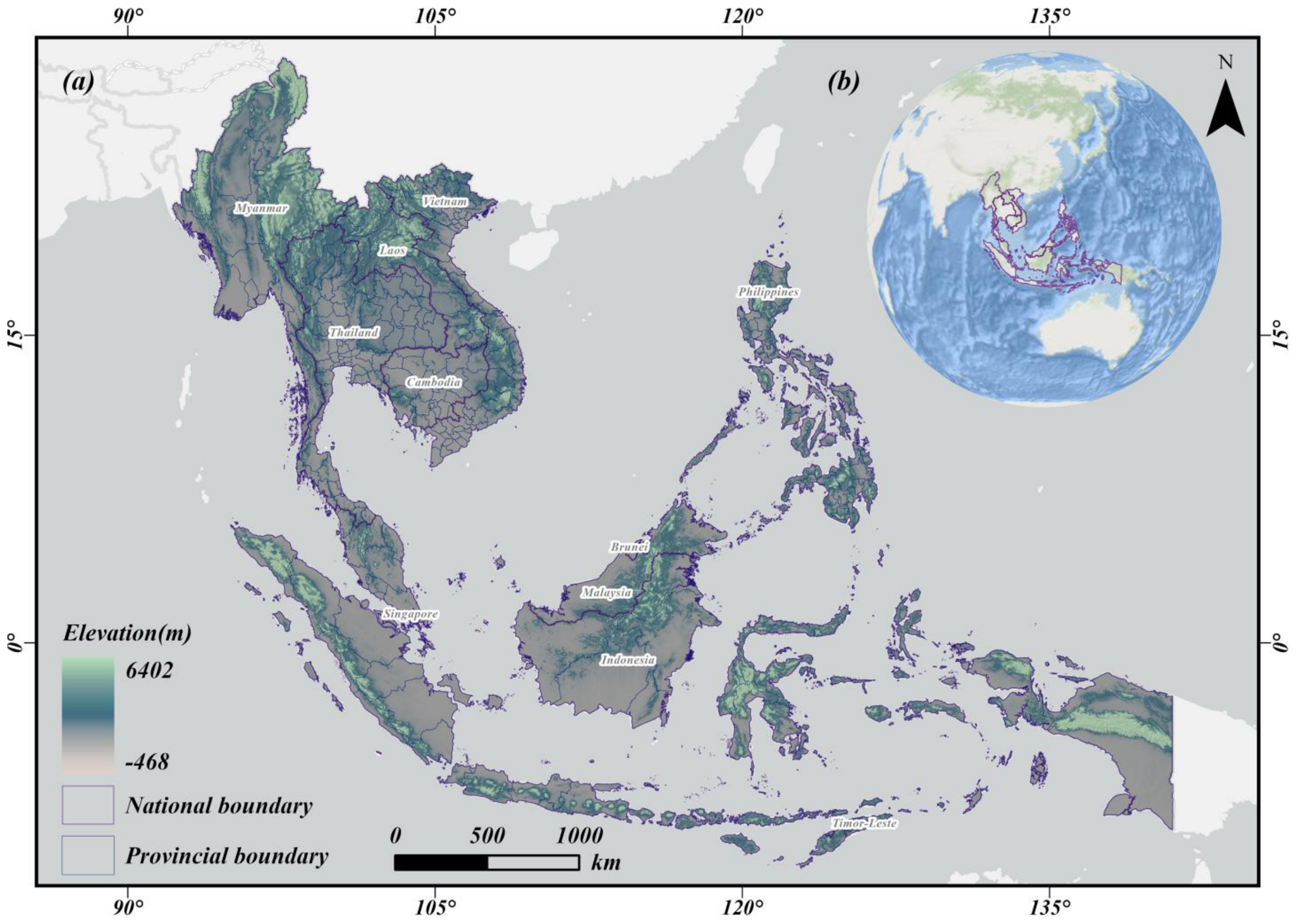
This study looks at the 11 ASEAN member states: Brunei, Cambodia, Indonesia, Laos, Malaysia, Myanmar, the Philippines, Singapore, Thailand, Vietnam, and Timor-Leste. The region covers approximately 4.5 million km² and has a population of over 700 million, making it one of the most dynamic areas in the Global South for urbanisation and industrial relocation. The study area is divided into two main subregions: the Indochina Peninsula and the Malay Archipelago, and it includes a diverse range of landforms such as alluvial plains, karst formations, mountainous and hilly regions, volcanic island chains, and extensive coastal areas. With the exception of some elevated inland regions, the area’s predominant climate is defined by tropical rainforests and tropical monsoons, which are characterised by consistently high temperatures, high humidity, significant rainfall, and regionally distinct wet and dry seasons. Furthermore, Southeast Asia’s complex biogeographical history has resulted in extraordinarily diverse and highly endemic biological communities, cementing its status as one of the world’s leading biodiversity hotspots [41]. This study integrates and standardises first-level administrative boundary data from 11 countries to achieve regional comparability while maintaining the spatial resolution required for policy-oriented analysis, yielding an analytical framework consisting of 351 provinces, states, municipalities, or equivalent administrative units. This framework is used to investigate the spatiotemporal evolution of coupling coordination between urbanisation and the natural environment from 2014 to 2024. The study area and topographic context are shown in Figure 1.

2.2. Data Sources and Preprocessing

Processing massive amounts of imagery, time-series compositing, and interannual comparisons are all components of large-scale remote sensing monitoring across the transnational Southeast Asian region, putting a high demand on data storage and processing power. To ensure consistency and reproducibility in the data processing workflow, all spatial data preprocessing, band calculations, and index construction in this study were performed using the Google Earth Engine (GEE) platform [42]. Given the study period’s regional development phases, six pivotal years—2014, 2016, 2018, 2020, 2022, and 2024—were chosen to demonstrate the sequential evolution of the interrelationship between urbanisation and the ecological environment in Southeast Asia.

In order to create the Improved Remote Sensing Ecological Index (IRSEI), the MODIS/061 MOD09A1 surface reflectance product and the MOD11A2 land surface temperature product were employed for the ecological environment dimension. Due to the region’s constant cloud cover and vast water bodies, cloud, cloud-shadow, and low-quality pixels were initially eliminated using quality control flags, and water masks were used to reduce the impact of large water areas on ecological indicator extraction. Median compositing was then used to generate annual cloud-free remote sensing mosaics. Using these datasets, ecological variables such as the Enhanced Vegetation Index (EVI), Land Surface Temperature (LST), Wetness Component (WET), Normalised Difference Built-up and Soil Index (NDBSI), and Bare Soil Index (SI) were extracted and synthesised using principal component analysis to create the IRSEI, a comprehensive metric of regional ecological environmental quality.

Monthly VIIRS nightlight data was used to create an annual nightlight time series for the urbanisation dimension. The spatial distribution of nighttime light intensity for each target year was obtained by suppressing outliers, removing background noise, and combining annual data. At the first-level administrative unit scale, the ratio of illuminated pixels and the mean nighttime light intensity were computed and then combined to create the Composite Nighttime Light Index (CNLI), which is used to delineate urbanisation levels at a transnational subnational scale.

2.3. IRSEI Construction

The conventional Remote Sensing Ecological Index (RSEI) consists of four elements—greenness, wetness, heat, and dryness—and has been commonly utilised in regional ecological quality assessments [43,44]. Nonetheless, due to Southeast Asia’s distinct geographical and climatic characteristics, including a prominent tropical monsoon climate, dense vegetation, and extensive coastlines, certain indicators within the traditional RSEI framework—such as the easily saturated Normalised Difference Vegetation Index (NDVI) and the snow-centric Normalised Difference Snow Index (NDSI)—are not entirely appropriate for this region. Thus, this study developed an Improved Remote Sensing Ecological Index (IRSEI) for tropical coastal environments using the Google Earth Engine (GEE) platform (

Table 1. Basic IRSEI Indicators and Their Ecological Implications.

Indicators	Meaning	Ecological Effect	Description
EVI	Enhanced Vegetation Index	+	Represents vegetation growth conditions and ecological restoration capacity
WET	Wetness Component	+	Reflects surface moisture conditions and hydrothermal characteristics
LST	Land Surface Temperature	−	Represents thermal environmental stress at the land surface
NDBSI	Normalized Difference Built-up and Soil Index	−	Reflects the disturbance intensity of built-up land and bare soil
SI	Bare Soil Index	−	Represents soil exposure and surface dryness characteristics

Note: “+” denotes a positive ecological effect, whereas “−” denotes a negative ecological effect.

).

To reduce subjective bias caused by manual weighting, this study used principal component analysis (PCA) to integrate multiple indicators and determine their weights, allowing each ecological factor’s information contribution to be fully represented [19,44]. Prior to performing PCA, all indicators were truncated from 1% to 99% to remove dimensional discrepancies and reduce the impact of extreme outliers. The initial principal component (PC1) accounts for the vast majority of the variance in the original variables. PC1 was inversely transformed (1-PC1) when its loading direction was negatively correlated with ecological conditions. EVI and WET typically improve ecological quality, while LST, NDBSI, and SI have negative impacts. The ultimate IRSEI was then calculated as follows:

To ensure comparability across the six target years, PCA was implemented at the whole-study-area level for each year rather than separately for individual countries or sub-regions. Because the sign of a principal component is mathematically arbitrary, the PC1 direction was standardised according to the ecological meaning of the loadings: EVI and WET were expected to contribute positively to ecological quality, whereas LST, NDBSI and SI were expected to contribute negatively. For each year, the loading direction was checked against this rule and, when the sign was reversed, PC1 was transformed as 1-PC1. Thus, interannual IRSEI comparability depends on a consistent ecological sign convention rather than on the raw eigenvector sign. Potential sub-regional variation in loading structures is acknowledged as a source of uncertainty, but no sub-regional PCA was applied because it would reduce cross-country comparability.

$$\mathrm{I}\mathrm{R}\mathrm{S}\mathrm{E}{\mathrm{I}}_0=\mathrm{P}\mathrm{C}1\left[\mathrm{f}\right(\mathrm{E}\mathrm{V}\mathrm{I},\mathrm{W}\mathrm{E}\mathrm{T},\mathrm{L}\mathrm{S}\mathrm{T},\mathrm{N}\mathrm{D}\mathrm{B}\mathrm{S}\mathrm{I},\mathrm{S}\mathrm{I}\left)\right]$$

(1)

$$\mathrm{I}\mathrm{R}\mathrm{S}\mathrm{E}\mathrm{I}={\displaystyle \frac{\mathrm{I}\mathrm{R}\mathrm{S}\mathrm{E}{\mathrm{I}}_0-\mathrm{I}\mathrm{R}\mathrm{S}\mathrm{E}{\mathrm{I}}_{0\_\mathrm{m}\mathrm{i}\mathrm{n}}}{\mathrm{I}\mathrm{R}\mathrm{S}\mathrm{E}{\mathrm{I}}_{0\_\mathrm{m}\mathrm{a}\mathrm{x}}-\mathrm{I}\mathrm{R}\mathrm{S}\mathrm{E}{\mathrm{I}}_{0\_\mathrm{m}\mathrm{i}\mathrm{n}}}}$$

(2)

The IRSEI ranges from 0 to 1. A higher value indicates better ecological and environmental quality. This study divides the IRSEI into five categories based on previous research: Excellent (0.8–1), Good (0.6–0.8), Moderate (0.4–0.6), Fair (0.2–0.4), and Poor (0–0.2) [44,45]. This study aggregates the pixel-scale IRSEI to provincial, prefectural, municipal, or equivalent administrative levels to identify the ecological and environmental conditions of various administrative units in each target year.

2.4. CNLI Construction

This study utilises the Composite Nighttime Light Index (CNLI) to assess the spatial-material dimension of urbanisation in a given region, more precisely urban expansion and built-up development intensity rather than demographic urbanisation in the strict sense [46,47]. This index is based on monthly VIIRS nighttime light data and takes into account both the spatial spread of illuminated surfaces and the intensity of socioeconomic activity. It has a strong correlation and consistency with urbanisation levels, making it widely used for monitoring built-up development. After aggregating data at the first administrative unit, this study computes the proportion of illuminated pixel area and normalised average light intensity before constructing the CNLI. This index is primarily made up of two components: the proportion of illuminated area (LAP) and the normalised average light intensity. The specific calculation formulas are as follows:

$$\mathrm{L}\mathrm{A}{\mathrm{P}}_{\mathrm{i}}={\displaystyle \frac{{\mathrm{N}}_{\mathrm{l}\mathrm{i}\mathrm{t},\mathrm{i}}}{{\mathrm{N}}_{\mathrm{t}\mathrm{o}\mathrm{t}\mathrm{a}\mathrm{l},\mathrm{i}}}}$$

(3)

In the formula, ${\mathrm{N}}_{\mathrm{l}\mathrm{i}\mathrm{t},\mathrm{i}}$ represents the number of illuminated pixels within the i-th administrative unit, and ${\mathrm{N}}_{\mathrm{t}\mathrm{o}\mathrm{t}\mathrm{a}\mathrm{l},\mathrm{i}}$ represents the total number of pixels in that unit. This indicator reflects the extent to which urban development has expanded within administrative units.

$$\mathrm{N}\mathrm{A}{\mathrm{P}}_{\mathrm{i}}={\displaystyle \frac{\raisebox{1ex}{$\sum \mathrm{D}{\mathrm{N}}_{\mathrm{i}}$}\!\left/ \!\raisebox{-1ex}{${\mathrm{N}}_{\mathrm{l}\mathrm{i}\mathrm{t},\mathrm{i}}$}\right.}{\mathrm{D}{\mathrm{N}}_{\mathrm{m}\mathrm{a}\mathrm{x}}}}$$

(4)

where $\sum \mathrm{D}{\mathrm{N}}_{\mathrm{i}}$ represents the sum of the light intensity values of all illuminated pixels within the i-th administrative unit, ${\mathrm{N}}_{\mathrm{l}\mathrm{i}\mathrm{t},\mathrm{i}}$ represents the number of illuminated pixels, and $\mathrm{D}{\mathrm{N}}_{\mathrm{m}\mathrm{a}\mathrm{x}}$ represents the set maximum light intensity value. This indicator reflects the intensity of regional development and the level of light concentration.

A further limitation of CNLI is potential high-end saturation. In highly urbanised units, especially Singapore and central metropolitan districts, both the illuminated-area proportion (LAP) and normalised average light intensity (NAP) may approach their upper bounds. In such cases, CNLI can still distinguish broadly high-intensity built-up development from lower-intensity areas, but its ability to detect marginal growth or intra-urban differences is compressed. The resulting CCD values for high-end units should therefore be interpreted as broad coordination levels rather than precise measures of continuing urbanisation intensity.

$$\mathrm{C}\mathrm{N}\mathrm{L}{\mathrm{I}}_{\mathrm{i}}=\mathrm{L}\mathrm{A}{\mathrm{P}}_{\mathrm{i}}\times \mathrm{N}\mathrm{A}{\mathrm{P}}_{\mathrm{i}}$$

(5)

where represents the Composite Nighttime Lighting Index (CNLI) for the i-th administrative unit. A higher value indicates stronger nighttime-light intensity and illuminated-area coverage, which this study interprets as higher built-up development intensity. Because CNLI cannot directly measure migration, land tenure, functional mix, or institutional urban status, references to urbanisation in the empirical sections should be understood as remote-sensing-based urban expansion unless otherwise specified.

2.5. Coupling Coordination Degree Model

The equal-weight setting is a baseline sustainability assumption rather than an empirical claim that the two subsystems always have identical policy importance. It was adopted because the research question concerns coordination between urban development and ecological quality, and because privileging either subsystem would embed an a priori policy preference into the CCD calculation. Alternative weights would mainly affect units with a large imbalance between CNLI and IRSEI; therefore, the weighting scheme is treated as part of the uncertainty and robustness assessment rather than as an immutable parameter.

The Coupling and Coordination Degree (CCD) model typically consists of two indicators: coupling degree and coordination degree. The coupling degree quantifies the intensity of interactions and mutual influences among multiple systems, indicating the strength of their dynamic interconnections; the coordination degree evaluates whether these systems establish a positive interaction and synergistic development based on coupling, revealing the system’s overall level of coordinated evolution. This model effectively depicts the mutual constraints, interdependencies, and synergistic development states among various subsystems, making it a popular tool for studying the relationship between urbanisation and the ecological environment, as well as a critical tool for evaluating a region’s overall balanced development [45]. Despite this, this paper uses the Coupling and Coordination Degree Model to conduct a quantitative analysis of the ecological environment’s interaction with urbanisation. The specific calculation formula is as follows:

$$\mathrm{C}=2\times {[{\displaystyle \frac{\mathrm{U}\left(\mathrm{X}\right)\times \mathrm{E}\left(\mathrm{Y}\right)}{{\left(\mathrm{U}\right(\mathrm{X})+\mathrm{E}(\mathrm{Y}\left)\right)}^2}}]}^2$$

(6)

$$\mathrm{T}=\mathrm{i}\times \mathrm{U}\left(\mathrm{X}\right)+\mathrm{j}\times \mathrm{E}\left(\mathrm{Y}\right)$$

(7)

$$\mathrm{C}\mathrm{C}\mathrm{D}=\sqrt{\mathrm{C}\times \mathrm{T}}$$

(8)

where C represents the degree of coupling; the higher the value of C, the stronger the interaction between IRSEI and CNLI. $\mathrm{U}\left(\mathrm{X}\right)$ and $\mathrm{E}\left(\mathrm{Y}\right)$ represent the CNLI and IRSEI values for each city, respectively. T represents the comprehensive evaluation score, which effectively reflects the synergy between CNLI and IRSEI. $\mathrm{i}$ and j are the weighting coefficients for CNLI and IRSEI, respectively. Given the importance of the ecological environment and urbanisation in urban development, i = j = 0.5. CCD denotes the coupling coordination degree between IRSEI and CNLI, with a range between [0, 1]. According to previous research [48], CCD is classified into five levels (

Table 2. The classification levels of the CCD.

CCD Value	Levels
$0<\mathrm{C}\mathrm{C}\mathrm{D}\le 0.2$	Serious unbalanced
$0.2<\mathrm{C}\mathrm{C}\mathrm{D}\le 0.3$	Moderate unbalanced
$0.3<\mathrm{C}\mathrm{C}\mathrm{D}\le 0.4$	Basically balanced
$0.4<\mathrm{C}\mathrm{C}\mathrm{D}\le 0.55$	Moderate balanced
$0.55<\mathrm{C}\mathrm{C}\mathrm{D}\le 1$	High balanced

).

2.6. Correlation Analysis

The Spearman rank correlation test is a nonparametric technique that uses variable ranks to determine monotonic correlation [49]. In contrast to the traditional Pearson correlation, this method is more robust against outliers, can effectively handle nonlinear monotonic relationships, and is not dependent on the data following a normal distribution [50]. The fundamental principle entails converting the original data to a rank-order sequence and then computing the correlation coefficient, which reveals the consistency of hierarchical rankings among variables rather than the extent of linear correlation. The formula for the Spearman rank correlation coefficient is as follows:

$$\mathsf{\rho }=1-{\displaystyle \frac{6{\displaystyle {\sum }_{\mathrm{i}=1}^{\mathrm{n}}}{\mathrm{d}}_{\mathrm{i}}^2}{\mathrm{n}({\mathrm{n}}^2-1)}}$$

(9)

In the formula, ${\mathrm{d}}_{\mathrm{i}}$ represents the difference in ranks between the two variables for the i-th sample, and $\mathrm{n}$ represents the sample size. The value of $\mathsf{\rho }$ ranges from −1 to 1; a positive value indicates a positive monotonic correlation, while a negative value indicates a negative monotonic correlation. The larger the absolute value, the stronger the correlation.

This study employs the Coupling Coordination Degree (CCD) of each provincial-level unit as the dependent variable and identifies seven explanatory variables: Built-up Area Index (BUI), logarithm of population density (lnPOPD), elevation (DEM), forest cover (FORC), forest loss rate (FORL), annual mean temperature (TEM), and annual precipitation (PRE). Utilising provincial-level samples from 2014, 2016, 2018, 2020, 2022, and 2024, this study aims to ascertain the direction and magnitude of the relationship between the driving factors and the coordination level, thereby offering preliminary insights for future geographic detector analysis. The variables and data sources are summarised in

Table 3. Driving Factors of Coupling Coordination in Southeast Asia.

Category	Factor	Variable Definition	Data Source
Urban Development	Built-up Area Ratio (BUI)	Proportion of built-up and impervious surface pixels relative to the total area of each provincial unit (%)	MODIS MCD12Q1 (V061)
Population Distribution	Logarithm of Population Density (lnPOPD)	Natural logarithm of resident population density at the provincial level (original unit: persons/km2)	WorldPop
Topographic Characteristics	Mean Elevation (DEM)	Average elevation within each provincial administrative unit (m)	SRTM GL1 (30 m)
Ecological Background	Forest Coverage Rate (FORC)	Proportion of forest area (IGBP classes 1–5) relative to the total area of each provincial unit (%)	MODIS MCD12Q1 (V061)
Ecological Disturbance	Forest Loss Rate (FORL)	Proportion of forest loss area relative to the baseline forest extent in 2000 (%)	Hansen Global Forest Change (v1.11)
Climatic Conditions	Mean Annual	Annual mean air temperature at 2 m height within each provincial unit (°C)	ECMWF ERA5-Land
Climatic Conditions	Annual Precipitation (PRE)	Annual cumulative precipitation within each provincial unit (mm/yr)	CHIRPS Daily

.

2.7. Geographical Detector

Geostatistics is a statistical technique used to detect spatial heterogeneity and understand the underlying mechanisms [51]. In contrast to conventional regression analysis, this method has the following advantages: (1) it eliminates the need to address multicollinearity among explanatory variables; (2) it does not rely on the assumption of linearity between the dependent variable and the explanatory variables; and (3) it can identify interaction effects among multiple factors [52]. The fundamental principle states that if the independent variable X has a significant effect on the dependent variable Y, their spatial distributions should be consistent; specifically, X’s spatial stratification can adequately account for Y’s spatial variance [53].

This study adopts the Optimal Parameter Geographic Detector (OPGD) approach [54], maximizing the explanatory power of factor detection by searching for the optimal combination among various discretization methods (equidistant method, quantile method, K-means clustering) and different numbers of layers (k = 3~8). Explanatory power is characterized by the q-value, calculated as follows:

$$\mathrm{q}=1-{\displaystyle \frac{{\displaystyle {\sum }_{\mathrm{h}=1}^{\mathrm{L}}}{\mathrm{N}}_{\mathrm{h}}{\mathsf{\sigma }}_{\mathrm{h}}^2}{\mathrm{N}{\mathsf{\sigma }}^2}}$$

(10)

In the equation, h = 1, …, L denotes the stratum numbers, where L is the total number of strata; Nh and N represent the sample sizes for the hth stratum and the entire study area, respectively; ${\mathsf{\sigma }}_{\mathrm{h}}^2$ and ${\mathsf{\sigma }}^2$ represent the variances of the dependent variable for the hth stratum and the entire study area, respectively. The q-value ranges from 0 to 1; a higher value indicates that the factor has a stronger explanatory power for the spatial variation in the dependent variable.

This study employs the Coupling Coordination Degree (CCD) of each provincial-level unit as the dependent variable, alongside seven factors as explanatory variables, to assess the explanatory power of each factor regarding the spatial variation in CCD. Interaction analysis assesses the joint impact of two factors on CCD, specifically to ascertain whether the interplay between factors X₁ and X₂ amplifies, diminishes, or is independent of one another. By evaluating the explanatory capacity of individual factors q(X₁) and q(X₂) against the explanatory capacity following hierarchical aggregation q(X₁∩X₂), the interaction between the two factors can be categorised into five types (

Table 4. Interaction Types and Descriptions.

Interaction Type	Decision Rule
Nonlinear weakening	q(X1∩X2) < Min(q(X1), q(X2))
Uni-enhance	Min(q(X1), q(X2)) < q(X1∩X2) < Max(q(X1), q(X2))
Bivariate enhancement	Max(q(X1), q(X2)) < q(X1∩X2) < q(X1) + q(X2)
Independence	q(X1∩X2) = q(X1) + q(X2)
Nonlinear enhancement	q(X1∩X2) > q(X1) + q(X2)

).

2.8. Uncertainty and Robustness Assessment

Because the workflow combines MODIS, VIIRS, WorldPop, SRTM, Hansen Global Forest Change, ERA5-Land, CHIRPS, and administrative-boundary data, uncertainty may arise from sensor noise, cloud and cloud-shadow contamination, water masking, temporal compositing, spatial resampling, cross-product resolution mismatch, provincial aggregation, index normalisation, PCA loading direction, and CCD weighting or threshold settings. This study therefore treats CNLI, IRSEI, and CCD as relative indicators of provincial-scale patterns rather than exact measurements of urbanisation or ecological quality.

To avoid overstating precision, uncertainty was addressed in a sensitivity-oriented and interpretation-oriented manner. First, data uncertainty was reduced through cloud, cloud-shadow, low-quality-pixel and water masking, annual median compositing, and outlier truncation. Second, index-construction uncertainty was controlled by applying a consistent regional PCA sign convention and by interpreting CNLI as a proxy for built-up development rather than complete demographic urbanisation. Third, model uncertainty was reported through explicit discussion of the equal-weight CCD assumption, potential CNLI saturation, OPGD discretisation, and spatial aggregation effects. These procedures do not replace full pixel-level error propagation, but they make the main sources of uncertainty explicit and reduce the risk of overinterpreting small numerical differences.

3. Empirical Results

3.1. Overall Temporal Changes in Urbanisation and the Ecological Environment

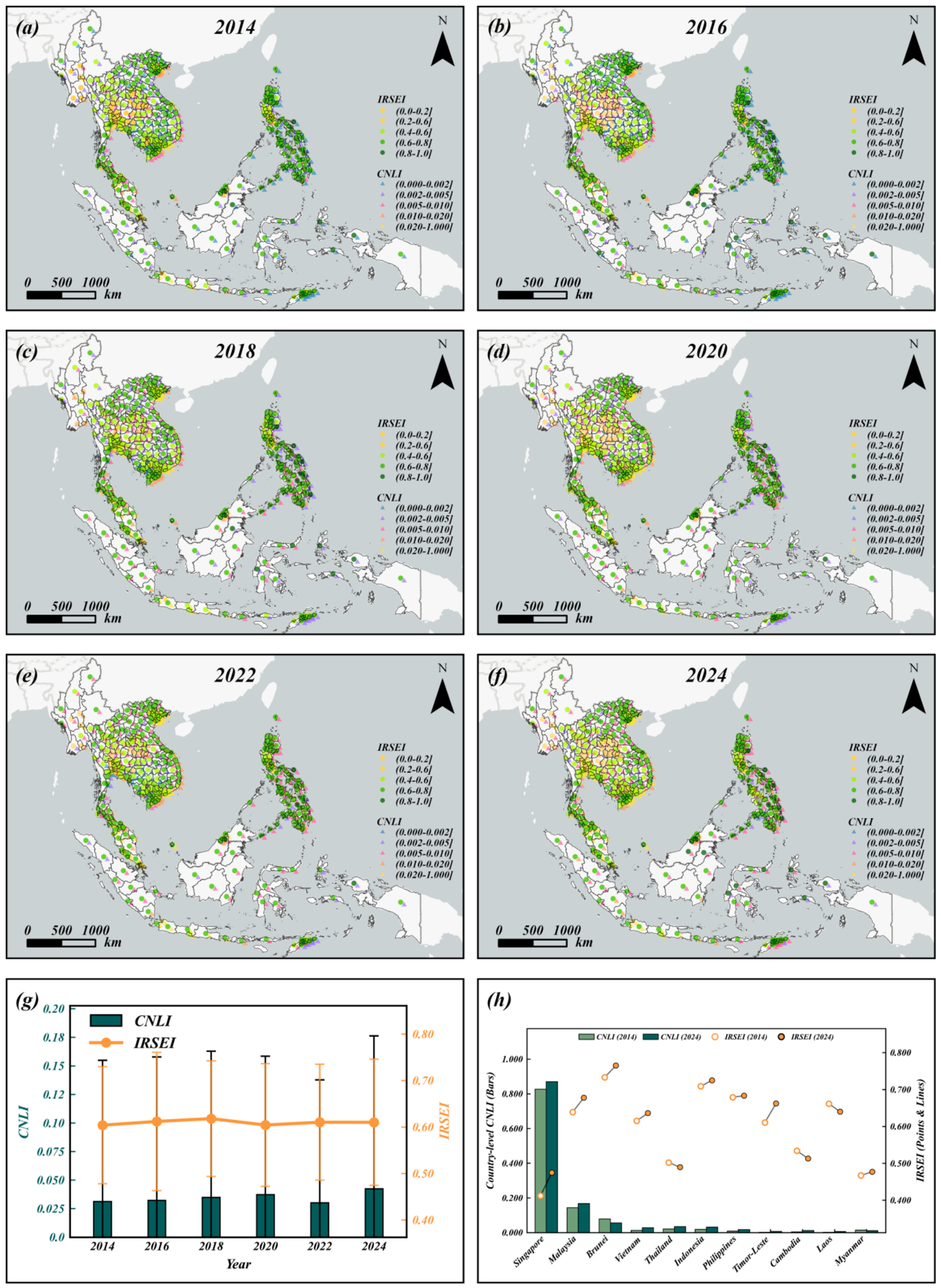
Between 2014 and 2024, CNLI-derived built-up development and the ecological environment in Southeast Asia experienced significantly divergent rates of change (Figure 2). The region’s urban expansion intensity continued to rise, while ecological and environmental quality remained relatively stable, indicating typical asynchronous changes. According to regional aggregate data, the average CNLI in Southeast Asia increased from 0.031 in 2014 to 0.042 in 2024, representing a 35.9% increase overall. In contrast, the average IRSEI increased marginally, from 0.604 to 0.610, representing a 1.0% increase. This means that, throughout the study period, the acceleration of built-up development and the increase in development intensity in Southeast Asia far outweighed improvements in ecological and environmental quality.

From a temporal standpoint, the CNLI predominantly displayed a variable upward trajectory throughout the study period. From 2014 to 2020, the regional average CNLI increased steadily from 0.031 to 0.037, indicating the persistent urbanisation in Southeast Asia; it experienced a minor decline to 0.030 in 2022, before reaching a peak of 0.042 in 2024. Conversely, the IRSEI consistently ranged from 0.60 to 0.62 between 2014 and 2024, attaining a maximum of 0.618 in 2018, declining to 0.604 in 2020, and later rebounding to approximately 0.610, exhibiting minimal overall variations (Figure 2g). This suggests that the ecological and environmental quality in Southeast Asia did not exhibit a notable improvement alongside urbanisation over the decade, but instead remained relatively stable.

The spatial patterns of CNLI and IRSEI demonstrate notable differences in their distributions (Figure 2a–f). Regions exhibiting elevated IRSEI values have historically been concentrated in the northern sector of the Indochinese Peninsula, the interiors of select Indonesian islands, and peripheral areas with relatively preserved ecological conditions. In contrast, high CNLI values are predominantly located in Singapore, the western coastline of the Malay Peninsula, Java, the Manila Metropolitan Area, and specific coastal and capital metropolitan regions. The spatial disjunction between regions of significant ecological value and areas of intense urbanisation suggests that urban development and the ecological environment in Southeast Asia have not established a synchronous diffusion pattern; instead, they largely display traits of functional differentiation and spatial segregation.

National-level differences further support this conclusion (Figure 2h). In 2024, Singapore’s CNLI was markedly superior to that of other nations, with Malaysia in second place, whereas Laos, Myanmar, and Cambodia exhibited comparatively low levels of urbanisation overall. Simultaneously, despite variations in IRSEI among nations, its overall volatility is considerably less than that of the CNLI. This suggests that the principal distinctions among Southeast Asian nations are predominantly in urbanisation levels rather than in the quality of the ecological environment itself. The degree of urbanisation in Southeast Asia increased markedly from 2014 to 2024, whereas the quality of the ecological environment exhibited only minor variations and modest enhancements, indicating that the rate of urban growth has substantially outpaced ecological improvement during the region’s development.

3.2. Spatial Patterns and Regional Gradient Variations in Coupling Coordination

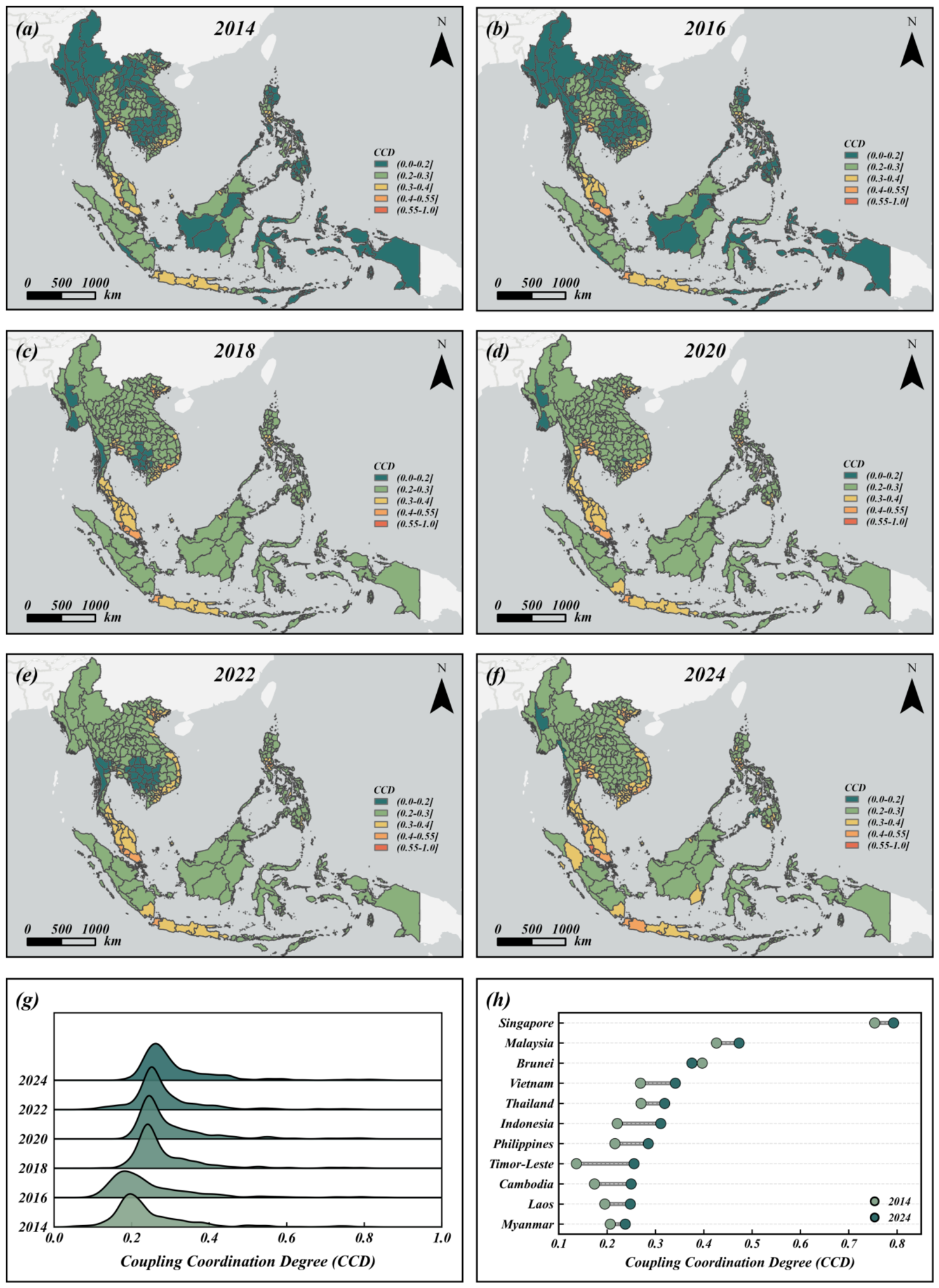
The preceding analysis elucidates the temporal attributes of urbanisation and the ecological environment; nonetheless, additional evaluation is required to ascertain whether the two progress in a synchronised fashion. This section employs the Coupling Coordination Degree (CCD) to delineate the intricate relationship between the two entities and their spatial configurations. From 2014 to 2024, the Coupling Coordination Degree (CCD) of urbanisation and the ecological environment in Southeast Asia displayed a generally fluctuating upward trajectory (Figure 3). The regional mean of the CCD rose from 0.250 in 2014 to 0.314 in 2024, reflecting a cumulative increase of 25.9% and signifying an enhancement in the regional coupling relationship. This enhancement mainly transpired within the low-to-medium coordination spectrum of “unbalanced” to “basically balanced,” indicating that the synergistic optimisation of urbanisation and the ecological environment in Southeast Asia is still largely incremental and has not yet established a pervasive, high-level coordination framework.

Improvements in regional CCD have transpired in phases: it was 0.250 in 2014, increased to 0.287 in 2018, and further to 0.299 in 2020; it subsequently decreased to 0.283 in 2022 and attained its peak value of 0.314 in 2024. The probability density distribution of the provincial CCD has shifted rightward over time (Figure 3g), signifying an enhancement in the coordination levels of the majority of provincial units. The distribution peak has consistently been centred in the 0.2–0.4 range, indicating that regional enhancement is predominantly manifested as a general upward shift among units at low-to-medium levels, rather than a comprehensive advancement to a high-coordination stage.

The CCD displays clear patterns of high-value clustering and low-value contiguity (Figure 3a–f). High-value regions are predominantly located in densely urbanised core areas, including the districts of Singapore, Kuala Lumpur, and Putrajaya in Malaysia, the Jakarta Capital Region in Indonesia, and the Manila Metropolitan Area in the Philippines; conversely, low-value regions are more extensively dispersed throughout Myanmar, Laos, Cambodia, East Timor, and specific peripheral provinces in Indonesia and the Philippines, illustrating significant spatial inequalities. In 2024, the provincial units exhibiting the highest coordination scores are predominantly situated in the central regions of Singapore and Malaysia (e.g., Singapore Central 0.849, East 0.821, North-East 0.813; and Malaysia’s Kuala Lumpur 0.791, Putrajaya 0.759), whereas those with the lowest scores are primarily found in the Philippines and Myanmar (e.g., Zamboanga Sibugay 0.183, Misamis Occidental 0.188, Mon 0.194, Magway 0.199).

The national average CCD across the 11 countries exhibits considerable stratification (Figure 3h). In 2024, Singapore had the highest average CCD (0.793), significantly higher than other countries; Malaysia (0.473) and Brunei (0.375) formed the second tier; Vietnam (0.341), Thailand (0.319), and Indonesia (0.311) are at an intermediate level; the Philippines (0.285), Timor-Leste (0.256), Cambodia (0.250), Laos (0.248), and Myanmar (0.237) are generally lower. A subsequent analysis of the extent of change indicates that regional enhancement is predominantly propelled by nations at the low-to-medium tier: Timor-Leste, Cambodia, and the Philippines exhibited substantial increases (+0.137, +0.085, and +0.076, respectively), whereas Singapore recorded a marginal increase (+0.004) and Brunei encountered a minor decline (−0.009), illustrating the relatively constrained potential for advancement among high-performing nations.

3.3. Transfer Pathways and Catch-Up Effects of Coupling-Driven Growth

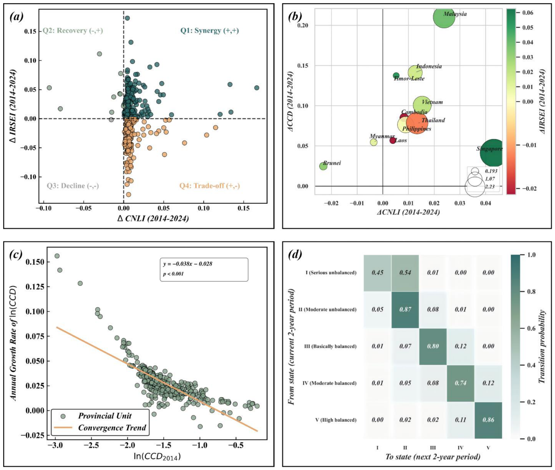
While the regional average CCD exhibits an upward trend, it is yet to be ascertained whether provincial units are experiencing similar advancements or if there is a phenomenon of convergence or divergence. This section utilises provincial-level incremental data from 2014 to 2024 to delineate the trends in urbanisation (ΔCNLI) and ecological environment (ΔIRSEI) into four quadrants, thereby characterising the internal dynamics of this coupled evolution. We thoroughly illustrate regional evolution pathways by incorporating national disparities, convergence relationships, and a hierarchical transition matrix (Figure 4).

CNLI-derived urban expansion and ecological-environmental changes in Southeast Asia demonstrate considerable asynchrony. Of the 351 provincial units, 205 (58.4%) are situated in the first quadrant (ΔCNLI > 0 and ΔIRSEI > 0), signifying concurrent advancements in built-up development and the ecological environment; 136 (38.7%) are positioned in the fourth quadrant (ΔCNLI > 0 and ΔIRSEI < 0), where urban expansion is coupled with deterioration in the ecological environment. The quantity of units in the second and third quadrants was minimal (9 units, representing 2.6%; and 1 unit, representing 0.3%, respectively). This pattern indicates that built-up development is a broader regional trend, while ecological and environmental responses demonstrate greater instability and spatial variability. These differences are consistent with a land-use transition perspective: some provinces appear to combine development with ecological restoration, whereas others experience expansion through conversion of agricultural land, forest margins, or peri-urban landscapes without sufficient ecological compensation.

A comparison of incremental changes at the national level further elucidates these disparities (Figure 4b). Certain nations have realised more significant advancements in CCD concurrent with increases in CNLI (e.g., Malaysia and Singapore have attained synergistic enhancements despite elevated urbanisation levels; Indonesia and Vietnam also exhibit considerable potential for synchronised progress during their urbanisation phases), whereas advancements in other countries are predominantly contingent upon incremental improvements from low baselines or are marked by inadequate urbanisation momentum and restricted coordinated enhancement. This signifies that diverse nations encounter distinct rates of development and challenges in reconciling urbanisation with ecological adaptation.

Subsequent convergence tests indicate that the enhancement in provincial CCD demonstrates notable catch-up traits from a low baseline (Figure 4c). The initial CCD from 2014 (log-transformed) demonstrates a negative regression coefficient when analysing the average annual growth rate from 2014 to 2024, suggesting that provincial units with lower initial coordination levels tend to show higher improvement rates throughout the study period. The hierarchical transition matrix demonstrates that the evolution displays significant path dependence (Figure 4d): the probabilities on the diagonal are markedly greater than those off-diagonal, and state transitions predominantly happen between adjacent levels, with minimal leapfrog transitions. This indicates that enhancements in regional coupling are more akin to gradual upward transitions than to abrupt changes.

The enhancement in coupling and coordination in Southeast Asia from 2014 to 2024 is chiefly attributed to ongoing advancements in low-to-medium coordination units, revealing a clear pattern of spatial divergence: certain areas have realised concurrent improvements in urbanisation and ecological conditions, while others confront ecological and environmental challenges amidst urban growth, thereby representing the principal tensions and policy trajectories in the region’s coupling evolution.

3.4. Test for Correlation Among Driving Factors

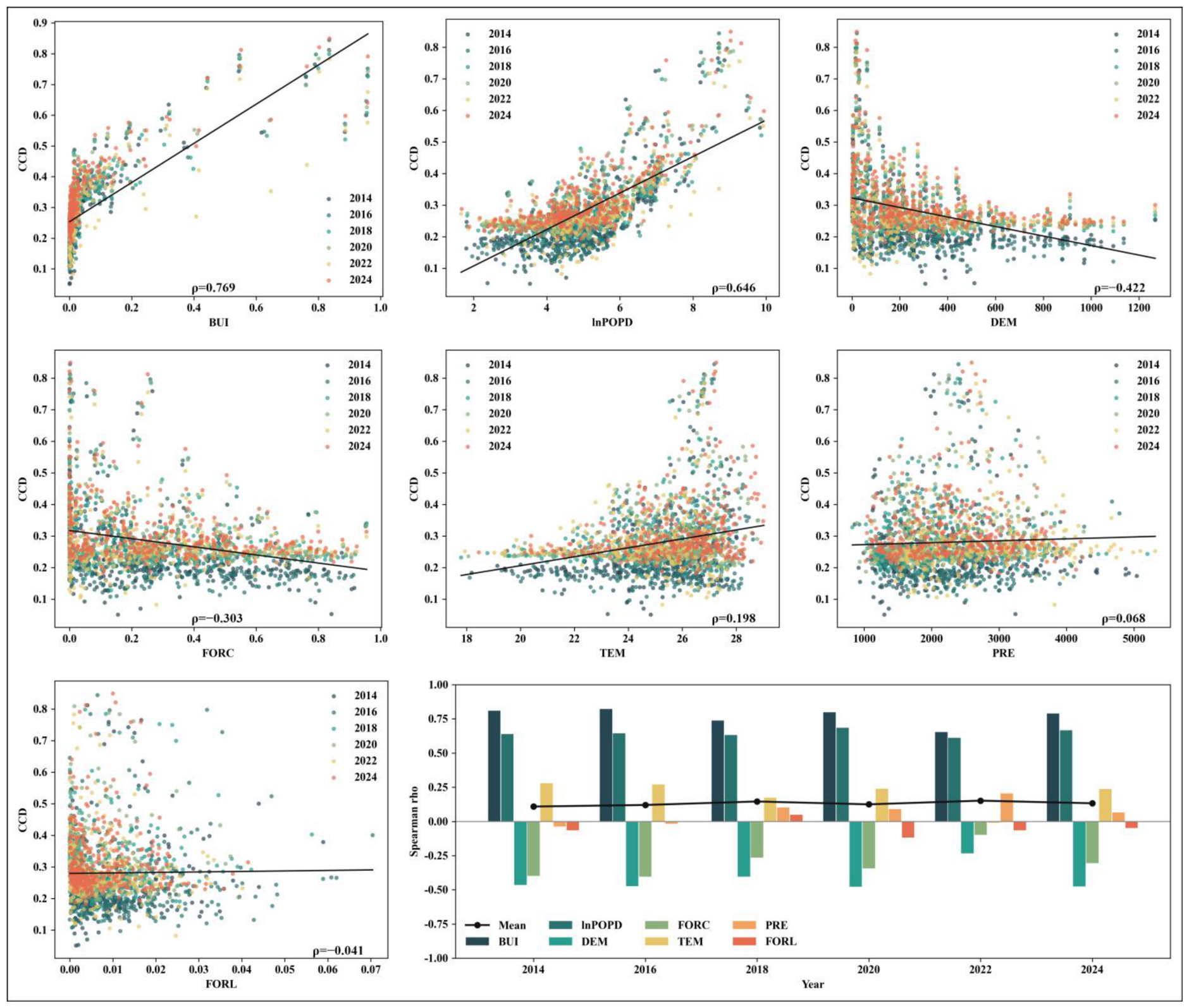
After identifying the two principal pathways of synergistic enhancement and trade-off, it is essential to examine the factors significantly correlated with CCD levels and their variations. This section seeks to elucidate the direction and intensity of the relationships between CCD and various driving factors, while also providing preliminary insights for subsequent geographic detector analysis. Utilising samples from 2014, 2016, 2018, 2020, 2022, and 2024, we performed Spearman’s rank correlation tests to determine the correlation coefficients ($\mathsf{\rho }$) between CCD and seven influencing factors (BUI, lnPOPD, DEM, FORC, FORL, PRE, TEM). Concurrently, we generated scatter plots differentiated by year and applied overall trend lines (Figure 5) to enable swift visual recognition of positive and negative correlations as well as interannual fluctuations.

Overall, there is a stronger correlation between human activity-related factors and CCD: BUI and lnPOPD generally exhibit positive correlations throughout all years, with comparatively higher correlation strengths, suggesting that an increase in CCD is frequently accompanied by the expansion of built-up land and population concentration. On the other hand, TEM typically shows a weak-to-moderate positive correlation, while the correlation between PRE and FORL is weaker and has more noticeable interannual fluctuations. DEM and FORC, on the other hand, primarily show negative correlations, indicating that topographic conditions and forest cover mitigate CCD changes to some extent. In order to perform a more thorough examination of the driving mechanisms from the viewpoints of spatial heterogeneity and factor interactions, this study also uses a geographic detector. It is crucial to note that correlation tests reflect statistical associations rather than causal relationships.

3.5. Factors Affecting CCDs Based on Geographical Detectors

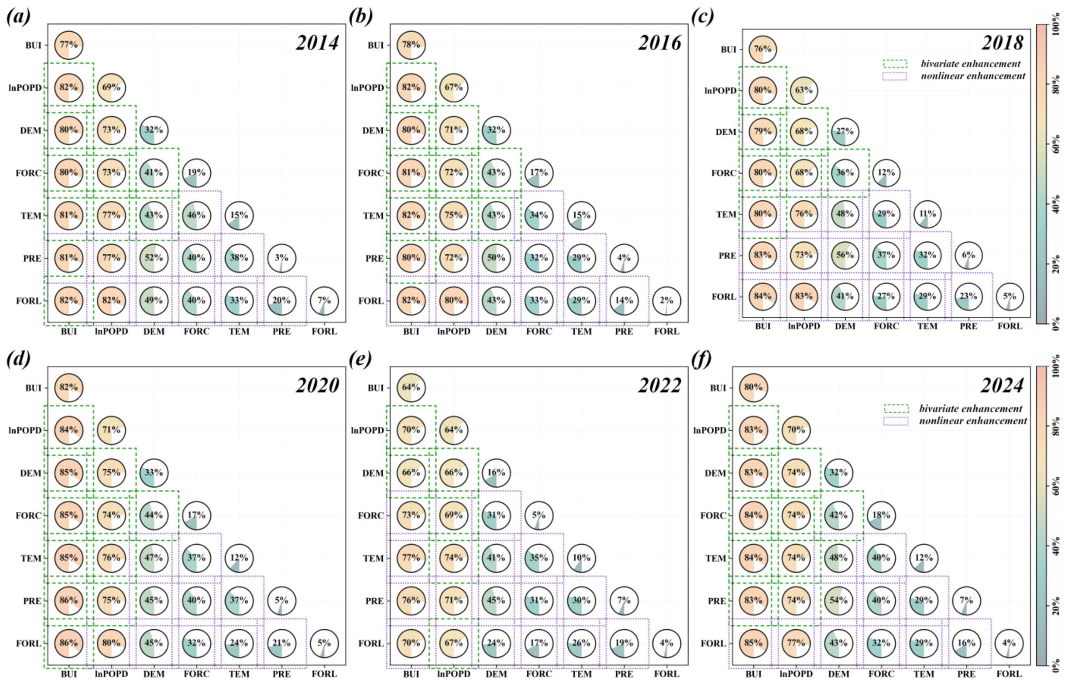
Correlation tests solely indicate statistical associations and are incapable of quantifying the explanatory influence of individual factors or their interactive effects on the spatial variation in CCD. This section utilises the Geographical Detector to perform factor contribution and interaction analyses.

Table 5. Single-factor detection results in Southeast Asia from 2014 to 2024.

Influencing Factors	2014	2016	2018	2020	2022	2024	Average
BUI	0.769	0.777	0.761	0.821	0.637	0.804	0.761
lnPOPD	0.689	0.672	0.632	0.706	0.639	0.701	0.673
DEM	0.319	0.325	0.271	0.325	0.161	0.322	0.287
FORC	0.186	0.170	0.119	0.174	0.053	0.177	0.147
TEM	0.147	0.150	0.108	0.119	0.099	0.121	0.124
PRE	0.030	0.044	0.055	0.054	0.067	0.066	0.053
FORL	0.067	0.018	0.049	0.050	0.036	0.036	0.043

Note: Values are q-statistics from OPGD factor detection and represent explanatory power rather than regression coefficients. No significance symbols are shown because statistical significance is not reported in the table body.

reports q-values from single-factor detection at the provincial level; a higher q-value indicates stronger explanatory power for the spatial variation in CCD, while statistical significance should be interpreted separately from the magnitude of q. The findings indicate that CCD is primarily structured by the spatial imprint of built-up development and population concentration: BUI had the highest explanatory power across all periods (q = 0.637–0.821, average q = 0.761), while lnPOPD consistently ranked second (q = 0.632–0.706, average q = 0.673). DEM had a moderate influence (q = 0.161–0.325, average q = 0.287), suggesting that terrain still constrains settlement location, infrastructure provision, and ecological exposure. FORC and TEM had weaker but non-negligible explanatory power (average q = 0.147 and 0.124), whereas PRE and FORL had lower individual q-values (average q = 0.053 and 0.043). These values imply that climatic and ecological disturbance variables may operate less as isolated drivers than as contextual conditions that amplify or constrain the effects of built-up expansion.

Further interaction analysis (Figure 6) shows that the combined effects of multiple factors improve the explanatory power for CCD. During the 2014–2024 period, bivariate and nonlinear enhancement were the two interaction types shown in Figure 6, indicating that no single factor fully explains the spatial differentiation of CCD. Across the six panels, interactions involving BUI and lnPOPD generally had the greatest explanatory power. The maximum interaction q-values were 0.82 in 2014 (BUI∩lnPOPD, BUI∩FORL, and lnPOPD∩FORL), 0.82 in 2016 (BUI∩lnPOPD, BUI∩TEM, and BUI∩FORL), 0.84 in 2018 (BUI∩FORL), 0.86 in 2020 (BUI∩PRE and BUI∩FORL), 0.77 in 2022 (BUI∩TEM), and 0.85 in 2024 (BUI∩FORL). This suggests that, at the provincial level, there is a significant synergistic effect between the urbanisation process and climatic conditions (PRE/TEM) as well as ecological disturbances (FORL), and that spatial variation in CCD is more consistent with the comprehensive logic of “urbanisation-driven, nature-constrained, and climate/disturbance-synergistically amplified” interactions.

The comparatively weaker or negative role of natural factors should be interpreted in relation to Southeast Asia’s spatial structure. Mountainous and forested provinces often have stronger ecological endowments but lower nighttime-light intensity, lower population concentration, and weaker infrastructure provision; this combination can reduce CCD under a framework that jointly evaluates CNLI and IRSEI. Temperature and precipitation also do not determine coordination directly. Instead, they shape the risk context in which land conversion occurs, including heat stress, flood exposure, water availability, vegetation stress, and the resilience of coastal or forest ecosystems. This explains why TEM, PRE and FORL gain importance in interaction detection even when their single-factor q-values are relatively low.

4. Discussion

4.1. The Relationship Between IRSEI, CNLI, and CCD

The relationship between urbanisation and the natural environment has long been a focus of research into regional sustainable development. Previous research has produced conflicting results: rapid urban growth may result in ecological risks and environmental pressures [34,55,56], but urban development may also support ecological-economic coordination by increasing economic efficiency, infrastructure provision, and governance capacity [36,37]. This study argues that these positions are not mutually exclusive. Whether urbanisation improves or degrades ecological coordination depends on the form of land-use transition, the location of expansion, the ecological baseline that is converted, and the capacity of regional governance to internalise environmental costs. Therefore, the results should not be interpreted as showing that urbanisation is inherently beneficial; rather, they show that some forms of built-up development are better coordinated with ecological management than others. This interpretation is consistent with recent evidence that urbanisation may first reduce eco-efficiency or carbon-emissions efficiency and later improve it only after governance, technological progress, and agglomeration benefits become strong enough [38,39].

This study provides new evidence at the transnational scale by showing that the positive correlation between CNLI and CCD (Figure 5) mainly reflects the co-location of built-up development, population concentration, infrastructure intensity, and administrative capacity. In mature metropolitan cores such as Singapore, Kuala Lumpur-Putrajaya, Jakarta, and Manila, high CNLI values may coexist with higher CCD because these areas have stronger service systems, environmental investment, and regulatory capacity. However, the same positive relationship cannot be generalised to all urbanising regions. The negative correlation between FORC and CCD does not imply that forest conservation prevents coordinated development. It is more likely due to structural covariation among provincial spatial types: marginal mountainous areas with high forest cover often have low CNLI, weak infrastructure, and limited administrative capacity, which lowers CCD within the coupling framework. As a result, coordination depends not only on ecological endowment but also on whether land development is governed, compact, and ecologically compensated.

Another key finding from path differentiation analysis (Figure 4a) is that built-up development is more widespread, whereas ecological responses are more unstable. Trade-off regions reveal a structural tension between “improved coordination” and “ecological pressure”: CCD can increase when CNLI rises, even if ecological quality deteriorates, because the model captures coupled development intensity as well as ecological conditions. This reinforces the need to interpret CCD together with ΔCNLI and ΔIRSEI rather than using CCD alone as a sustainability score. From a land-use perspective, trade-off provinces are likely to be places where peri-urban housing, industrial estates, transport infrastructure, coastal tourism, or plantation-related settlement expansion convert agricultural or forested land faster than ecological restoration and regulation can respond. Policymakers should therefore link urban expansion control, ecological compensation, and peri-urban land management instead of treating urbanisation and environmental protection as separate agendas.

The 136 trade-off units are not a minor residual group, but account for 38.7% of all provincial units. The quadrant and national aggregation results suggest that these trade-offs are especially relevant in provinces undergoing rapid built-up expansion from low or medium baseline coordination, including parts of the Philippines, Thailand, Cambodia, Indonesia, and peripheral metropolitan or corridor zones. Such areas are often exposed to industrial relocation, road and port development, tourism-led coastal construction, plantation-related settlement expansion, and the conversion of agricultural or forest margins. Therefore, the positive CNLI-CCD association should not be read as evidence that urbanisation automatically improves sustainability; it is conditional on whether urban growth is compact, serviced, climate-resilient, and ecologically compensated.

4.2. Coordination in Southeast Asia

The spatial hierarchy revealed in this study (Figure 3) provides support for a territorial-development interpretation of coupling coordination. Core regions, such as Singapore, the Kuala Lumpur-Putrajaya metropolitan area, the Jakarta Capital Region, and the Manila Metropolitan Area, can maintain relatively high coordination under high-intensity built-up development because they concentrate economic functions, infrastructure networks, fiscal resources, and environmental governance capacity. These advantages allow core regions to absorb some ecological pressures through investment in water management, green infrastructure, waste treatment, and planning controls. At the same time, these metropolitan areas may externalise part of their environmental footprint through land, food, energy, labour, and material flows to surrounding rural or peri-urban regions, which means that high local CCD should be interpreted within a broader city-region system rather than as an isolated local achievement [3,7].

This interpretation is particularly important for Singapore and other high-urbanisation cores. Because nighttime-light indicators may saturate at the upper end, the very high CCD values in these units should be read as evidence of a high-level coordination state at the provincial scale, not as a precise ranking of marginal urbanisation intensity within already fully urbanised spaces. Saturation may slightly compress differences among high-end units and may understate additional development intensity after the CNLI has approached its upper range.

In contrast, Myanmar, Laos, Cambodia, Timor-Leste, and certain peripheral provinces in the Philippines and Indonesia have yet to establish a virtuous cycle between built-up development and ecological management, resulting in persistently low levels of coordination. However, convergence test results (Figure 4c) show that units with lower initial coordination levels improved more quickly during the study period, exhibiting a distinct “low-baseline catch-up” pattern. This finding implies that the potential for improving regional coordination lies primarily in developing countries and underdeveloped regions, but catch-up should not be equated with indiscriminate land conversion. A more sustainable pathway would combine basic infrastructure provision with compact settlement growth, protection of agricultural land, restoration of degraded forest margins, and stronger provincial land-use governance.

The state transition matrix (Figure 4d) shows that changes in coordination levels occur primarily between adjacent levels, with leapfrog transitions being uncommon. This suggests that regional coupling in Southeast Asia will evolve through incremental optimisation rather than rapid short-term leaps. Moving forward, policymakers should prioritise transnational and transregional collaborative governance mechanisms that connect metropolitan cores, peri-urban transition zones, agricultural hinterlands, and ecological conservation areas. While accelerating the catch-up of regions with low coordination, these mechanisms should also prevent regions with high coordination from experiencing development inertia lock-in, ecological-pressure rebound, or the displacement of environmental costs to surrounding rural territories.

4.3. Factors Affecting Coupling Coordination

Previous studies have primarily used GTWR, the barrier index model, or Tobit regression to analyse the coupled drivers of coordination [57,58,59], but these methods fail to effectively identify nonlinear interaction effects among factors. To address these shortcomings, this study introduces the Geographical Detector Model. The results of the single-factor detection (Table 5) show that factors related to built-up development and population concentration are the primary drivers shaping the spatial differentiation of CCD: BUI had the highest explanatory power across all periods, while lnPOPD consistently came in second. BUI should therefore be interpreted not simply as an “urbanisation variable” but as a land-conversion indicator reflecting the expansion of impervious and built-up surfaces. Topography (DEM) has moderate explanatory power, reflecting the persistent constraints of terrain on settlement distribution, infrastructure costs, and ecological sensitivity. Climatic factors and forest disturbances have weaker individual explanatory power, but their importance increases through interactions with built-up development.

The interaction analysis results (Figure 6) show that any combination of two factors produces either bivariate enhancement or nonlinear enhancement, and the strongest combinations almost always include BUI. This indicates that urban expansion amplifies the effects of population concentration, climate conditions, forest disturbance, and topographic constraints. The drivers behind growth are therefore not only local physical conditions but also broader development processes, including industrial relocation, metropolitan spillover, port and logistics development, tourism investment, transport-infrastructure expansion, and national or provincial land-development strategies. Although these institutional and economic drivers are not directly measured in the present model, the OPGD results are consistent with a broader theoretical framework of “land-conversion-driven, nature-constrained, and governance-mediated” coupling. Regional policy design should consequently shift from single-factor linear interventions to multi-factor collaborative governance, with climate adaptation, ecological conservation, land-conversion control, and urban–rural coordination embedded into spatial planning. Evidence on strategic interactions among regional governments also suggests that green innovation and environmental policy effects can spill over across administrative boundaries, reinforcing the need to consider governance-mediated coupling rather than only local physical drivers [60].

4.4. Land-Use Transitions, Peri-Urban Dynamics and Urban–Rural Linkages

A key mechanism behind asynchronous evolution is land-use transition at urban margins. In Southeast Asia, urban expansion rarely occurs only through compact infill inside existing urban cores. It also advances through suburban industrial estates, logistics corridors, peri-urban housing, tourism enclaves, new-town projects, and the conversion of rice fields, plantations, wetlands, secondary forests, and coastal ecosystems [3,4,7,10,11]. These processes create mosaic landscapes in which urban, rural, and ecological functions coexist. The CCD results align with this interpretation: high coordination is concentrated in mature metropolitan cores, whereas trade-off patterns are common in provinces where built-up development expands faster than ecological restoration, land-use control, or environmental-service provision.

Urban–rural linkages further explain why ecological outcomes diverge among provinces. Metropolitan demand for land, labour, food, energy, construction materials, tourism space, and infrastructure can shift environmental pressures beyond administratively defined urban cores. Conversely, rural landscapes and ecological assets support urban resilience through food supply, watershed regulation, flood retention, carbon storage, cooling, and biodiversity conservation [3,7,11,32]. Coupling coordination should therefore be interpreted as a territorial process shaped by flows across city-region systems, not merely as a local statistical relationship between nighttime lights and ecological indices.

This perspective has direct policy implications and suggests that policy packages should be differentiated by regional type. High-urbanisation/high-coordination cores, such as Singapore and mature metropolitan districts, should focus on maintaining ecological performance, avoiding ecological-pressure rebound, upgrading green-blue infrastructure, and reducing the displacement of environmental costs to surrounding rural or peri-urban areas. High-urbanisation/trade-off areas should prioritise strict land-conversion control, compact redevelopment, ecological compensation, flood- and heat-risk zoning, and environmental impact assessment for industrial, logistics, tourism, and transport-infrastructure projects. Low-urbanisation/low-coordination regions require basic services, infrastructure access, and compact settlement growth, but should avoid using extensive land conversion as the main development pathway. Ecologically sensitive low-urbanisation areas should preserve forest margins, wetlands, agricultural land, and watershed functions while using cross-regional compensation mechanisms to share the benefits and costs of conservation. Because BUI is the dominant driver and climatic factors amplify its effects, spatial planning should integrate built-up land quotas, climate-adaptation zoning, green-blue corridors, and urban–rural land governance rather than relying only on sectoral environmental measures.

4.5. Limitations of the Study

This research has certain limitations. First, the quantitative indicators for the ecological environment and built-up development are not yet complete. This study employs the IRSEI to assess ecological environmental quality; while it incorporates a bare soil index into the traditional RSEI to account for tropical coastal environments, it still fails to address critical dimensions such as air quality, biodiversity, habitat connectivity, water quality, and ecosystem-service flows [22]. In terms of urbanisation, the CNLI is primarily based on nighttime-light intensity and coverage, so it captures built-up development and socioeconomic light intensity more effectively than daytime industrial production, informal settlements, agricultural-dominated peri-urban economies, or legal-administrative urban status. Future research could combine multi-source data, such as Sentinel-5P atmospheric products, high-resolution land-use classification, building footprints, road networks, and settlement morphology metrics, to create a more comprehensive indicator system. Second, the selection of driving factors is based on natural background conditions and population-spatial factors, with limited representation of institutional environment, land-use regulation, fiscal capacity, infrastructure investment, economic structure, and environmental policy [29,59]. Southeast Asian countries differ significantly in terms of governance capacity, environmental regulation stringency, and enforcement efficiency; these factors may have a significant impact on coordinated evolution and should be included in future analytical frameworks. Third, the uncertainty assessment in this study is sensitivity-oriented rather than a full pixel-level error-propagation analysis. Remote-sensing data quality, cloud contamination, coastal water masking, PCA loading direction, OPGD discretisation, and CCD weighting may still influence the magnitude of results, even when major patterns remain robust. Finally, the provincial administrative-unit scale used in this study may obscure internal spatial heterogeneity and peri-urban gradients, and the correlation analysis and geographical detectors show statistical associations rather than strict causal relationships. Future research could combine finer spatial scales, field validation, quasi-experimental designs, dynamic simulations, and scenario projections to validate causal mechanisms and evaluate policy alternatives for land-use transition and urban–rural governance. In addition, high-end nighttime-light saturation may reduce the ability of CNLI to distinguish marginal changes among already highly urbanised units, and potential spatial variation in PCA loading structures may influence local IRSEI values even though a consistent regional sign convention was applied. These limitations reinforce the need to interpret the results as regional-scale coordination patterns rather than exact local measurements.

5. Conclusions

In light of Southeast Asia’s rapid urbanisation, this study investigates the asynchronous evolution of ecological environmental quality and the spatial-material dimension of urbanisation from a land-use transition perspective. Provincial-level evolution trajectories show notable divergence, but overall regional coupling and coordination have gradually improved according to long-term quantitative measurements. The results indicate that built-up area expansion and population concentration are the main drivers of CCD differentiation, while climatic conditions, ecological disturbances, and topographic constraints produce strong nonlinear interactive amplification effects. These findings suggest that the central policy issue is not urban growth itself, but the form, location, and governance of land conversion. Trade-off development regions should simultaneously strengthen ecological investment, control peri-urban land conversion, protect agricultural and forest margins, and pursue compact built-up development. Underdeveloped regions with substantial potential for synergistic improvement require cross-regional collaborative governance mechanisms that support basic infrastructure and public services without replicating ecologically damaging expansion pathways. High-coordination nations and metropolitan cores need to prevent ecological-pressure rebound, development inertia lock-in, and the displacement of environmental costs to surrounding rural territories. In specific planning implementation, policy formulation should move from single-factor linear interventions to multi-factor collaborative governance, embedding climate adaptation, ecological protection, urban–rural linkages, and land-use transition management into regional spatial planning. In the end, this strategy will optimise the overall ecological advantages and development quality of complex transnational areas.

References

1. Li, M.; Cao, Y.; Dai, J.; Song, J.; Liang, M. A comprehensive review of urban expansion and its driving factors. Land 2025, 14, 1534. [Google Scholar] [CrossRef] [Scilit]
2. Seto, K.C.; Güneralp, B.; Hutyra, L.R. Global forecasts of urban expansion to 2030 and direct impacts on biodiversity and carbon pools. Proc. Natl. Acad. Sci. USA 2012, 109, 16083–16088. [Google Scholar] [CrossRef] [Scilit] [PubMed]
3. Seto, K.C.; Reenberg, A.; Boone, C.G.; Fragkias, M.; Haase, D.; Langanke, T.; Marcotullio, P.; Munroe, D.K.; Olah, B.; Simon, D. Urban land teleconnections and sustainability. Proc. Natl. Acad. Sci. USA 2012, 109, 7687–7692. [Google Scholar] [CrossRef] [Scilit] [PubMed]
4. McGee, T.G. The emergence of desakota regions in Asia: Expanding a hypothesis. In The Extended Metropolis: Settlement Transition in Asia; Ginsburg, N., Koppel, B., McGee, T.G., Eds.; University of Hawaii Press: Honolulu, HI, USA, 1991; pp. 3–25. [Google Scholar]
5. Haddad, N.M.; Brudvig, L.A.; Clobert, J.; Davies, K.F.; Gonzalez, A.; Holt, R.D.; Lovejoy, T.E.; Sexton, J.O.; Austin, M.P.; Collins, C.D.; et al. Habitat fragmentation and its lasting impact on Earth’s ecosystems. Sci. Adv. 2015, 1, e1500052. [Google Scholar] [CrossRef] [Scilit] [PubMed]
6. Costanza, R.; de Groot, R.; Sutton, P.; van der Ploeg, S.; Anderson, S.J.; Kubiszewski, I.; Farber, S.; Turner, R.K. Changes in the global value of ecosystem services. Glob. Environ. Change 2014, 26, 152–158. [Google Scholar] [CrossRef] [Scilit]
7. Tacoli, C. Rural-urban interactions: A guide to the literature. Environ. Urban. 1998, 10, 147–166. [Google Scholar] [CrossRef]
8. Estoque, R.C.; Ooba, M.; Avitabile, V.; Hijioka, Y.; DasGupta, R.; Togawa, T.; Murayama, Y. The future of Southeast Asia’s forests. Nat. Commun. 2019, 10, 1829. [Google Scholar] [CrossRef] [Scilit] [PubMed]
9. Nandy, S.; Kushwaha, S.P.S.; Dadhwal, V.K. Carbon storage and sequestration in Southeast Asian urban clusters under future land cover change scenarios (2015–2050). Front. Environ. Sci. 2023, 11, 1105759. [Google Scholar] [CrossRef] [Scilit]
10. Allen, A. Environmental planning and management of the peri-urban interface: Perspectives on an emerging field. Environ. Urban. 2003, 15, 135–147. [Google Scholar] [CrossRef] [Scilit]
11. Simon, D. Urban environments: Issues on the peri-urban fringe. Annu. Rev. Environ. Resour. 2008, 33, 167–185. [Google Scholar] [CrossRef]
12. United Nations, Department of Economic and Social Affairs, Population Division. World Urbanization Prospects: The 2018 Revision; United Nations: New York, NY, USA, 2019; Available online: https://population.un.org/wup/ (accessed on 15 July 2026).
13. Fajary, F.R.; Lee, H.S.; Kubota, T.; Bhanage, V.; Pradana, R.P.; Nimiya, H.; Putra, I.D.G.A. Comprehensive spatiotemporal evaluation of urban growth, surface urban heat island, and urban thermal conditions on Java island of Indonesia and implications for urban planning. Heliyon 2024, 10, e33708. [Google Scholar] [CrossRef] [Scilit] [PubMed]
14. Paradis, E. Forest gains and losses in Southeast Asia over 27 years: The slow convergence towards reforestation. For. Policy Econ. 2021, 122, 102332. [Google Scholar] [CrossRef] [Scilit]
15. Hansen, M.C.; Potapov, P.V.; Moore, R.; Hancher, M.; Turubanova, S.A.; Tyukavina, A.; Thau, D.; Stehman, S.V.; Goetz, S.J.; Loveland, T.R.; et al. High-resolution global maps of 21st-century forest cover change. Science 2013, 342, 850–853. [Google Scholar] [CrossRef] [Scilit] [PubMed]
16. Zhao, M.; Zhou, Y.; Li, X.; Cheng, W.; Zhou, C.; Ma, T.; Li, M.; Huang, K. Mapping urban dynamics (1992–2018) in Southeast Asia using consistent nighttime light data from DMSP and VIIRS. Remote Sens. Environ. 2020, 248, 111980. [Google Scholar] [CrossRef] [Scilit]
17. Xu, H.; Wang, Y.; Guan, H.; Shi, T.; Hu, X. Detecting ecological changes with a remote sensing based ecological index (RSEI) produced time series and change vector analysis. Remote Sens. 2019, 11, 2345. [Google Scholar] [CrossRef] [Scilit]
18. Sun, C.; Li, J.; Liu, Y.; Cao, L.; Zheng, J.; Yang, Z.; Ye, J.; Li, Y. Ecological quality assessment and monitoring using a time-series remote sensing-based ecological index (ts-RSEI). GISci. Remote Sens. 2022, 59, 1793–1816. [Google Scholar] [CrossRef] [Scilit]
19. Zheng, Z.; Wu, Z.; Chen, Y.; Guo, C.; Marinello, F. Instability of remote sensing based ecological index (RSEI) and its improvement for time series analysis. Sci. Total Environ. 2022, 814, 152595. [Google Scholar] [CrossRef] [Scilit] [PubMed]
20. Wang, J.; Li, H.; Wang, J.; Zhao, L.; Li, X.; Fan, W.; Chen, J. Continuous remote sensing ecological index (CRSEI): A novel approach for multitemporal monitoring of eco-environmental changes on large scale. Ecol. Indic. 2023, 154, 110739. [Google Scholar] [CrossRef] [Scilit]
21. Karimi Firozjaei, M.; Fathololoumi, S.; Kiavarz, M.; Biswas, A.; Homaee, M.; Alavipanah, S.K. Land Surface Ecological Status Composition Index (LSESCI): A novel remote sensing-based technique for modeling land surface ecological status. Ecol. Indic. 2021, 123, 107375. [Google Scholar] [CrossRef] [Scilit]
22. Liu, P.; Ren, C.; Yu, W.; Ren, H.; Xia, C. Exploring the ecological quality and its drivers based on annual remote sensing ecological index and multisource data in Northeast China. Ecol. Indic. 2023, 154, 110589. [Google Scholar] [CrossRef] [Scilit]
23. Lu, F.; Zhang, C.; Cao, H.; Wang, X.; Zheng, T.; Huang, Z. Assessment of ecological environment quality and their drivers in urban agglomeration based on a novel remote sensing ecological index. Ecol. Indic. 2025, 170, 113104. [Google Scholar] [CrossRef] [Scilit]
24. Ma, Z.; Zhang, P. Understanding how digital infrastructure construction could promote sustainable development. Sustain. Cities Soc. 2024, 117, 105977. [Google Scholar] [CrossRef] [Scilit]
25. Falah, N.; Falah, N.; Solis-Guzman, J.; Marrero, M. An indicator-based framework of circular cities focused on sustainability dimensions and sustainable development goal 11 obtained using machine learning and text analytics. Sustain. Cities Soc. 2025, 121, 106219. [Google Scholar] [CrossRef] [Scilit]
26. Jing, T.; Wang, H.; Yang, Y.; Jin, Y.; Yu, W.; Zhong, Y. Achieving sustainable development in coastal cities: Exploring the synergies between urban resilience and high-quality development. Sustain. Cities Soc. 2026, 136, 107112. [Google Scholar] [CrossRef] [Scilit]
27. Ariken, M.; Zhang, F.; Liu, K.; Fang, C.; Kung, H.T. Coupling coordination analysis of urbanisation and eco-environment in Yanqi Basin based on multi-source remote sensing data. Ecol. Indic. 2020, 114, 106331. [Google Scholar] [CrossRef] [Scilit]
28. Tian, Y.; Zhou, D.; Jiang, G. Conflict or coordination? Multiscale assessment of the spatio-temporal coupling relationship between urbanisation and ecosystem services: The case of the Jingjinji Region, China. Ecol. Indic. 2020, 117, 106543. [Google Scholar] [CrossRef] [Scilit]
29. Zeng, P.; Wei, X.; Duan, Z. Coupling and coordination analysis in urban agglomerations of China: Urbanisation and ecological security perspectives. J. Clean. Prod. 2022, 365, 132730. [Google Scholar] [CrossRef] [Scilit]
30. Li, X.; Lu, Z.; Hou, Y.; Zhao, G.; Zhang, L. The coupling coordination degree between urbanisation and air environment in the Beijing (Jing)-Tianjin (Jin)-Hebei (Ji) urban agglomeration. Ecol. Indic. 2022, 137, 108787. [Google Scholar] [CrossRef] [Scilit]
31. Wan, H.; He, G.; Li, B.; Zeng, J.; Cai, Y.; Shen, X.; Yang, Z. Coupling coordination relationship between urbanisation and water environment in China. J. Clean. Prod. 2024, 472, 143423. [Google Scholar] [CrossRef] [Scilit]
32. Zhao, X.; Tan, S.; Li, Y.; Khan, S. Quantitative analysis of local coupling and telecoupling mechanism between urbanisation and ecological environment quality based on multi-source remote sensing data. Ecol. Indic. 2025, 173, 113345. [Google Scholar] [CrossRef] [Scilit]
33. Li, J.; Cui, D.; Bilal, I. Revealing the spatiotemporal dynamics and coupling coordination between urbanisation and ecological environment quality in the Aksu Region, Xinjiang. Ecol. Indic. 2025, 179, 114163. [Google Scholar] [CrossRef] [Scilit]
34. Fang, C.; Liu, H.; Wang, S. The coupling curve between urbanisation and the eco-environment: China’s urban agglomeration as a case study. Ecol. Indic. 2021, 130, 108107. [Google Scholar] [CrossRef] [Scilit]
35. Fang, X.; Shi, X.; Phillips, T.K.; Du, P.; Gao, W. The coupling coordinated development of urban environment towards sustainable urbanisation: An empirical study of Shandong Peninsula, China. Ecol. Indic. 2021, 129, 107864. [Google Scholar] [CrossRef] [Scilit]
36. Lei, X.; Liu, H.; Li, S.; Luo, Q.; Cheng, S.; Hu, G.; Wang, X.; Bai, W. Coupling coordination analysis of urbanisation and ecological environment in Chengdu-Chongqing urban agglomeration. Ecol. Indic. 2024, 161, 111969. [Google Scholar] [CrossRef] [Scilit]
37. Zou, C.; Zhu, J.; Lou, K.; Yang, L. Coupling coordination and spatiotemporal heterogeneity between urbanisation and ecological environment in Shaanxi Province, China. Ecol. Indic. 2022, 141, 109152. [Google Scholar] [CrossRef] [Scilit]
38. Yuan, X.; Nie, Y.; Zeng, L.; Lu, C.; Yang, T. Exploring the Impacts of Urbanization on Eco-Efficiency in China. Land 2023, 12, 687. [Google Scholar] [CrossRef] [Scilit]
39. Yang, L.; Liang, Z.; Yao, W.; Zhu, H.; Zeng, L.; Zhao, Z. What Are the Impacts of Urbanisation on Carbon Emissions Efficiency? Evidence from Western China. Land 2023, 12, 1707. [Google Scholar] [CrossRef] [Scilit]
40. Brenner, N.; Schmid, C. Towards a new epistemology of the urban? City 2015, 19, 151–182. [Google Scholar] [CrossRef] [Scilit]
41. Struebig, M.J.; Lee, J.S.H.; Deere, N.J.; Gevaña, D.T.; Ingram, D.J.; Lwin, N.; Nguyen, T.; Santika, T.; Seaman, D.J.I.; Supriatna, J.; et al. Drivers and solutions to Southeast Asia’s biodiversity crisis. Nat. Rev. Biodivers. 2025, 1, 497–514. [Google Scholar] [CrossRef] [Scilit]
42. Gorelick, N.; Hancher, M.; Dixon, M.; Ilyushchenko, S.; Thau, D.; Moore, R. Google Earth Engine: Planetary-scale geospatial analysis for everyone. Remote Sens. Environ. 2017, 202, 18–27. [Google Scholar] [CrossRef] [Scilit]
43. Wang, Z.; Chen, T.; Zhu, D.; Jia, K.; Plaza, A. RSEIFE: A new remote sensing ecological index for simulating the land surface eco-environment. J. Environ. Manag. 2023, 326, 116851. [Google Scholar] [CrossRef] [Scilit] [PubMed]
44. Xu, H. A remote sensing index for assessment of regional ecological changes. China Environ. Sci. 2013, 33, 889–897. [Google Scholar] [CrossRef]
45. Li, J.; Tian, Y. Assessment of ecological quality and analysis of influencing factors in coal-bearing hilly areas of northern China: An exploration of human mining and natural topography. Land 2024, 13, 1067. [Google Scholar] [CrossRef] [Scilit]
46. Zhuo, L.; Shi, P.J.; Chen, J.; Ichinose, T. Application of compound night light index derived from DMSP/OLS data to urbanisation analysis in China in the 1990s. Acta Geogr. Sin. 2003, 58, 893–902. [Google Scholar] [CrossRef]
47. Wang, Y.; Liu, Z.; He, C.; Xia, P.; Liu, Z.; Liu, H. Quantifying urbanization levels on the Tibetan Plateau with high-resolution nighttime light data. Geogr. Sustain. 2020, 1, 233–244. [Google Scholar] [CrossRef] [Scilit]
48. Zhang, X.; Fan, H.; Liu, F.; Lv, T.; Sun, L.; Li, Z.; Shang, W.; Xu, G. Coupling coordination between the ecological environment and urbanisation in the middle reaches of the Yangtze River urban agglomeration. Urban Clim. 2023, 52, 101698. [Google Scholar] [CrossRef] [Scilit]
49. Spearman, C. The proof and measurement of association between two things. Am. J. Psychol. 1904, 15, 72–101. [Google Scholar] [CrossRef] [Scilit] [PubMed]
50. Hauke, J.; Kossowski, T. Comparison of values of Pearson’s and Spearman’s correlation coefficients on the same sets of data. Quaest. Geogr. 2011, 30, 87–93. [Google Scholar] [CrossRef] [Scilit]
51. Wang, J.F.; Xu, C.D. Geodetector: Principle and prospective. Acta Geogr. Sin. 2017, 72, 116–134. [Google Scholar] [CrossRef]
52. Guo, B.; Wang, X.; Pei, L.; Su, Y.; Zhang, D.; Wang, Y. Identifying the spatiotemporal dynamic of PM2.5 concentrations at multiple scales using geographically and temporally weighted regression model across China during 2015–2018. Sci. Total Environ. 2021, 751, 141765. [Google Scholar] [CrossRef] [Scilit] [PubMed]
53. Wang, J.F.; Hu, Y. Environmental health risk detection with GeoDetector. Environ. Model. Softw. 2012, 33, 114–115. [Google Scholar] [CrossRef] [Scilit]
54. Song, Y.; Wang, J.; Ge, Y.; Xu, C. An optimal parameters-based geographical detector model enhances geographic characteristics of explanatory variables for spatial heterogeneity analysis: Cases with different types of spatial data. GISci. Remote Sens. 2020, 57, 593–610. [Google Scholar] [CrossRef] [Scilit]
55. Shi, Y.; Feng, C.C.; Yu, Q.; Han, R.; Guo, L. Contradiction or coordination? The spatiotemporal relationship between landscape ecological risks and urbanisation from coupling perspectives in China. J. Clean. Prod. 2022, 363, 132557. [Google Scholar] [CrossRef] [Scilit]
56. Luo, X.; Luan, W.; Li, Y.; Xiong, T. Coupling coordination analysis of urbanisation and the ecological environment based on urban functional zones. Front. Public Health 2023, 11, 1111044. [Google Scholar] [CrossRef] [Scilit] [PubMed]
57. Liu, L.; Guo, Y.; Li, Y.; Zhang, L. Examining the complex relationship between urbanisation and ecological environment in ecologically fragile areas: A case study in Southwest China. Front. Public Health 2024, 12, 1358051. [Google Scholar] [CrossRef] [Scilit] [PubMed]
58. Kan, D.; Ye, X.; Lyu, L.; Huang, W. Study on the coupling coordination between new-type urbanisation and water ecological environment and its driving factors: Evidence from Jiangxi Province, China. Int. J. Environ. Res. Public Health 2022, 19, 9998. [Google Scholar] [CrossRef] [Scilit] [PubMed]
59. Hu, J.; Zhang, J.; Li, Y. Exploring the spatial and temporal driving mechanisms of landscape patterns on habitat quality in a city undergoing rapid urbanisation based on GTWR and MGWR: The case of Nanjing, China. Ecol. Indic. 2022, 143, 109333. [Google Scholar] [CrossRef] [Scilit]
60. Li, C.; Shi, H.; Zeng, L.; Dong, X. How Strategic Interaction of Innovation Policies between China’s Regional Governments Affects Wind Energy Innovation. Sustainability 2022, 14, 2543. [Google Scholar] [CrossRef] [Scilit]
Figure 1. Topography of Southeast Asia. (a) Elevation and national/provincial boundaries across the 11-country study area; (b) location of the study area within Asia.
Land 15 01308 g001
Figure 2. Spatiotemporal Evolution of urbanisation and the Ecological Environment in Southeast Asia, 2014–2024. (af) Spatial distributions of CNLI and IRSEI for 2014, 2016, 2018, 2020, 2022, and 2024; (g) regional mean CNLI and IRSEI trajectories; (h) national-level CNLI and IRSEI comparison between 2014 and 2024.
Land 15 01308 g002
Figure 3. Spatiotemporal evolution of the Coupling Coordination Degree (CCD) in Southeast Asia from 2014 to 2024. (af) Spatial distributions of CCD for 2014, 2016, 2018, 2020, 2022, and 2024; (g) provincial CCD probability-density distributions; (h) national mean CCD comparison between 2014 and 2024.
Land 15 01308 g003
Figure 4. Asynchronous Characteristics and Dynamic Evolutionary Trajectories of urbanisation and Ecological Environments in Southeast Asia, 2014–2024. (a) Provincial ΔCNLI–ΔIRSEI quadrants; (b) national-level incremental changes; (c) convergence between initial CCD and subsequent growth; (d) transition matrix among CCD levels.
Land 15 01308 g004
Figure 5. Correlation analysis of driving factors in Southeast Asia from 2014 to 2024. Scatterplots are ordered from left to right and top to bottom as BUI, lnPOPD, DEM, FORC, TEM, PRE, and FORL; the bottom-right panel summarises the annual Spearman’s ρ values for the seven factors and their mean.
Land 15 01308 g005
Figure 6. Interaction detection results for Southeast Asia from 2014 to 2024. (a) 2014; (b) 2016; (c) 2018; (d) 2020; (e) 2022; (f) 2024.
Land 15 01308 g006