Article

Multi-Temporal Diagnosis and Uncertainty Analysis of Cropland Water Erosion in the Black Soil Region of Northeast China


School of Public Policy and Management, Guangxi University, Nanning 530004, China
*
Author to whom correspondence should be addressed.
Land 2026, 15(7), 1292; https://doi.org/10.3390/land15071292
Submission received: 22 June 2026 / Revised: 16 July 2026 / Accepted: 17 July 2026 / Published: 19 July 2026
(This article belongs to the Special Issue Synergistic Integration of Transport, Land, and Ecosystems)

Abstract

The black soil region of Northeast China is a key grain-production area where cropland water erosion threatens soil fertility and sustainability. We diagnosed cropland soil loss across six diagnostic years/time slices (2001, 2005, 2010, 2015, 2020, and 2024) using a Revised Universal Soil Loss Equation (RUSLE)-based remote-sensing workflow implemented in Google Earth Engine (GEE). Rainfall erosivity was derived from Climate Hazards Group InfraRed Precipitation with Station data (CHIRPS) daily precipitation, soil erodibility from SoilGrids, topography from the Shuttle Radar Topography Mission digital elevation model (SRTM DEM), vegetation cover from the Landsat normalized difference vegetation index (NDVI), and cropland extent from ESA WorldCover; alternative rainfall sources, cropland masks, and P-factor settings were used for sensitivity analyses. Under the slope-graded P-factor scenario, mean annual soil loss ranged from 1.60 to 3.07 t ha−1 yr−1, and the proportion of cropland exceeding T = 2 t ha−1 yr−1 ranged from 25.2% to 52.9%. Soil loss fluctuated among years because rainfall erosivity and cover-management effects partly counteracted each other. Risk was concentrated in sloping piedmont and hilly cropland, whereas broad plains were dominated by very slight and slight erosion. P-factor parameterization represented the largest structural uncertainty. The workflow provides regional screening evidence for field verification and conservation-practice assessment, rather than direct site-specific engineering prescriptions.

1. Introduction

Soil erosion by water is a cumulative form of land-surface degradation that thins cultivated soil, weakens aggregate stability and nutrient retention, and transfers sediment, carbon, nitrogen, and phosphorus through watersheds. It, therefore, links geomorphic change with food security, ecological security, and sustainable land management. Global assessments of land-use change, European soil loss, and erosion-related food-production risks frame water erosion in these coupled terms [1,2,3], while Montgomery emphasizes the intergenerational risk of soil loss exceeding soil formation [4]. Under global change, rising rainfall erosivity, intense storms, land-use transitions, and management shifts make erosion risk increasingly non-stationary [5,6,7]. Because erosion also aggravates phosphorus scarcity and agricultural productivity losses, diagnosis now extends from soil conservation to nutrient cycling and food-production security [8,9]. More broadly, recent studies of Chinese land systems show that digitalization, farmland-use transition, and urbanization are associated with changes in land-use efficiency and carbon-related environmental performance [10,11,12,13,14].
The black soil region of Northeast China is a high-latitude commodity grain-production region where sloping cropland erosion, cultivated-layer thinning, and black soil degradation converge. A standardized boundary dataset supports regional diagnosis, and previous empirical erosion-modeling, random-forest, geographic information system (GIS), and remote-sensing studies have linked erosion patterns with land-use change [15,16,17]. Recent studies on erosion-risk hotspots, dynamic change, and degradation mechanisms show that erosion clusters where relief, cropland connectivity, crop cover, and management interact [18,19,20]. Evidence on erosion rates, gully-related landscape structure, and long-term productivity losses further confirms that water erosion has direct agricultural consequences and cannot be represented adequately by one annual mean [21,22,23]. Here, erosion-risk hotspots refer to spatially concentrated cropland areas with relatively high model-estimated soil loss, gully-related degradation risk, or erosion-sensitive combinations of relief, land use, vegetation cover, and management conditions.
Empirical soil-loss models remain the dominant tools for large-area water erosion mapping. The Universal Soil Loss Equation (USLE) and Revised Universal Soil Loss Equation (RUSLE) combine rainfall erosivity, soil erodibility, slope length and steepness, cover-management, and support-practice effects in a multiplicative framework applied across climates, land-use systems, and scales [24,25,26]. Yet reviews of model reliability and soil erosion modeling show that RUSLE-type outputs depend strongly on factor construction, data sources, scale conversion, and parameter choices, and do not fully represent erosion mechanics [27,28]. Parsons et al., therefore, argue that empirical factor models should be interpreted within a process-informed framework rather than as complete physical representations [29]. This study consequently uses a RUSLE-based framework as a consistent relative diagnostic framework for cropland.
Factor construction is central to the diagnostic outcome. For the slope length and steepness factor, European LS studies, a Loess Plateau slope-length formulation, and LS accuracy evaluations show that terrain resolution, flow routing, and slope-length truncation can alter hillslope erosion potential [30,31,32]. For soil erodibility, global mapping, high-resolution Chinese mapping, and K-factor uncertainty studies indicate that equations based on sand, silt, clay, and organic carbon must be matched to regional soil-property data [33,34,35]. For cover management, European and global C-factor studies and grassland C-factor dynamics show that vegetation indices support continuous estimation, but normalized difference vegetation index (NDVI) thresholds, vegetation type, and seasonal weighting may introduce substantial differences [36,37,38].
Rainfall erosivity is the most direct climatic driver in RUSLE. Climate Hazards Group InfraRed Precipitation with Station data (CHIRPS) provides a stable long-term precipitation source, and Xie et al.’s daily rainfall erosivity model is operational for China, where high-frequency intensity observations are sparse [39,40]. Daily erosivity calculations, dynamic satellite precipitation products, and satellite-based applications in China and India show that satellite precipitation can support large-area erosivity estimation, but bias, temporal resolution, and extreme-rainfall capture still require sensitivity assessment [41,42,43]. Beguería et al. provide a basis for estimating erosivity from daily precipitation when sub-daily intensity data are unavailable [44]. Global high-temporal-resolution records, European monthly mapping, and Chinese re-examinations further show that rainfall source and temporal aggregation affect erosivity levels and spatial rankings [45,46,47].
Cover-management and support-practice factors describe human modulation of erosion and are among the most uncertain large-area inputs. Land-cover-based C-factor estimation, NDVI-based sensitivity analysis, and remote-sensing C-factor studies show that vegetation indices improve spatial continuity but require explicit bare-soil and dense-vegetation endmembers [48,49,50]. For the support-practice factor, global C/P analyses, European P-factor modeling, and improved RUSLE applications treat P as an empirical expression of management intensity [51,52,53]. Where pixel-level conservation-practice information is unavailable, scenario-based or stratified P settings are often unavoidable, and global evidence on conservation techniques warns that P scenarios should not be read as pixel-level observations of actual engineering measures [54]. Google Earth Engine (GEE) and multi-source raster workflows improve computational consistency and mapping efficiency [55,56,57,58], but they do not remove uncertainty in parameters, masks, or rainfall inputs.
In China and neighboring regions, erosion diagnosis is shifting from single-period mapping toward multi-scenario, multi-driver, and uncertainty-aware assessment. Future rainfall erosivity studies indicate that climate scenarios can alter spatial gradients and temporal trajectories [59,60]. Research on telecoupled cropland erosion, rainfall–soil–land-use pathways, and climate extremes and land-use interactions shows that erosion intensity usually emerges from multiple pressures rather than a single factor [61,62,63]. Nevertheless, three gaps remain for cropland water erosion in the black soil region: limited comparison of post-2001 time slices under one parameter framework, insufficient sensitivity analysis for rainfall source, cropland mask, and P-factor scenarios [64], and weak integration of slope band structure, cover dynamics, and endpoint relationships as joint geographic and statistical evidence. Model harmonization studies show that cross-scale and cross-scenario comparison helps separate robust patterns from convention-dependent outputs [64].
Field-based 137Cs measurements from 12 black-soil profiles reported a mean total erosion rate of 2.22 mm yr−1 and indicated that water erosion was dominant in the eastern part of the region [23]. Because these observations include processes and units that are not directly comparable with the present RUSLE estimates, they provide process-level context rather than validation of the modeled absolute soil-loss rates. The spatial pattern diagnosed here is consistent with this process understanding, but the present estimates should not be interpreted as direct field measurements. Instead, the contribution of this study is to extend field-based and local-scale understanding into a regional, multi-temporal, and uncertainty-aware RUSLE-GEE screening framework.
The analytical framework first harmonizes the black soil boundary and cropland mask, then parameterizes R, K, LS, C, and P factors in GEE, diagnoses soil loss for six time slices, and finally evaluates slope band patterns and uncertainty from P-factor scenarios, rainfall sources, cropland masks, and slope-unit settings.
This study develops a RUSLE-based diagnostic framework for cropland water erosion across six time slices in the black soil region of Northeast China. Using a consistent black soil boundary, cropland sampling frame, and RUSLE-factor convention, annual mean soil loss is estimated from CHIRPS precipitation, SoilGrids soil properties, Shuttle Radar Topography Mission (SRTM) terrain, Landsat vegetation indices, and the European Space Agency (ESA) WorldCover cropland mask; sensitivity analyses then replace key inputs with alternative rainfall products, an alternative cropland mask, and alternative P-factor scenarios. This design retains the interpretability of RUSLE while incorporating recent insights on remote-sensing C factors, P scenarios, rainfall-source uncertainty, and model reliability [27,65]. Rather than providing a final absolute estimate from one model, this study asks how cropland erosion intensity, the area exceeding the tolerance threshold, and spatial patterns changed from 2001 to 2024; how slope bands, cover-management, and support-practice scenarios jointly explain erosion risk; and whether the main conclusions remain stable when major inputs are replaced [66]. The results integrate geospatial and statistical evidence through multi-temporal maps, factor distributions, slope band statistics, sensitivity diagnostics, endpoint relationships, and R-C-SL diagnostic zoning.
The novelty of this study lies not in applying RUSLE alone, but in integrating six discrete temporal diagnostics (2001, 2005, 2010, 2015, 2020, and 2024), slope band stratification, P-factor scenario uncertainty, rainfall-source and cropland-mask sensitivity tests, and reproducible GEE implementation into one cropland-focused diagnostic workflow.

2. Study Area and Methods

2.1. Study Area and Data Sources

The study area was defined using the published boundary dataset of black and typical black soil regions in Northeast China, representing the major black soil belt of the region. The regional boundary follows the black soil region dataset released by Liu et al. [17]. The region lies in the mid-latitude temperate continental monsoon zone, where precipitation is concentrated mainly in the warm season under the influence of the summer monsoon. Across the six time slices considered in this study, precipitation inputs showed marked interannual variability. The terrain is dominated by the Songnen and Sanjiang plains and is generally flat, while steeper piedmont and hilly areas occur along the Greater and Lesser Khingan Mountains and the Changbai Mountains. These steeper areas were diagnosed by the model as having relatively higher water erosion risk. The main cropland sample was extracted from ESA WorldCover 2021 and used as the consistent cropland mask for the diagnostic statistics. The location of the study area, the black soil region boundary, and the major land-cover classes are shown in Figure 1.
The term “black soil region” is used here as a regional boundary concept rather than as an indication that every pixel within the study area is black soil. The analysis, therefore, focuses on cropland pixels within the published boundary, while soil texture and soil organic carbon variation are represented using gridded SoilGrids inputs.
From an erosion-process perspective, the broad Songnen and Sanjiang plains generally have low LS values, whereas piedmont and hilly transition zones along the Greater and Lesser Khingan Mountains and the Changbai Mountains contain more sloping cropland and can be more sensitive to runoff concentration. Freeze–thaw cycles and snowmelt may contribute to early-spring runoff, especially on sloping cropland and hilly margins, but these processes are not explicitly simulated by the rainfall-erosivity R factor used here.
The main datasets used in this study include CHIRPS Daily precipitation [39], SoilGrids soil properties, the Shuttle Radar Topography Mission digital elevation model (SRTM DEM) [67], Landsat surface reflectance [68], and the ESA WorldCover 2021 cropland mask, which were used to construct the R, K, LS, and C factors and the main cropland domain. Global Precipitation Measurement Integrated Multi-satellitE Retrievals for GPM (GPM IMERG), ECMWF Reanalysis v5 Land (ERA5-Land), and the Global Land Cover with Fine Classification System at 30 m (GLC FCS30D) were used for sensitivity analyses.
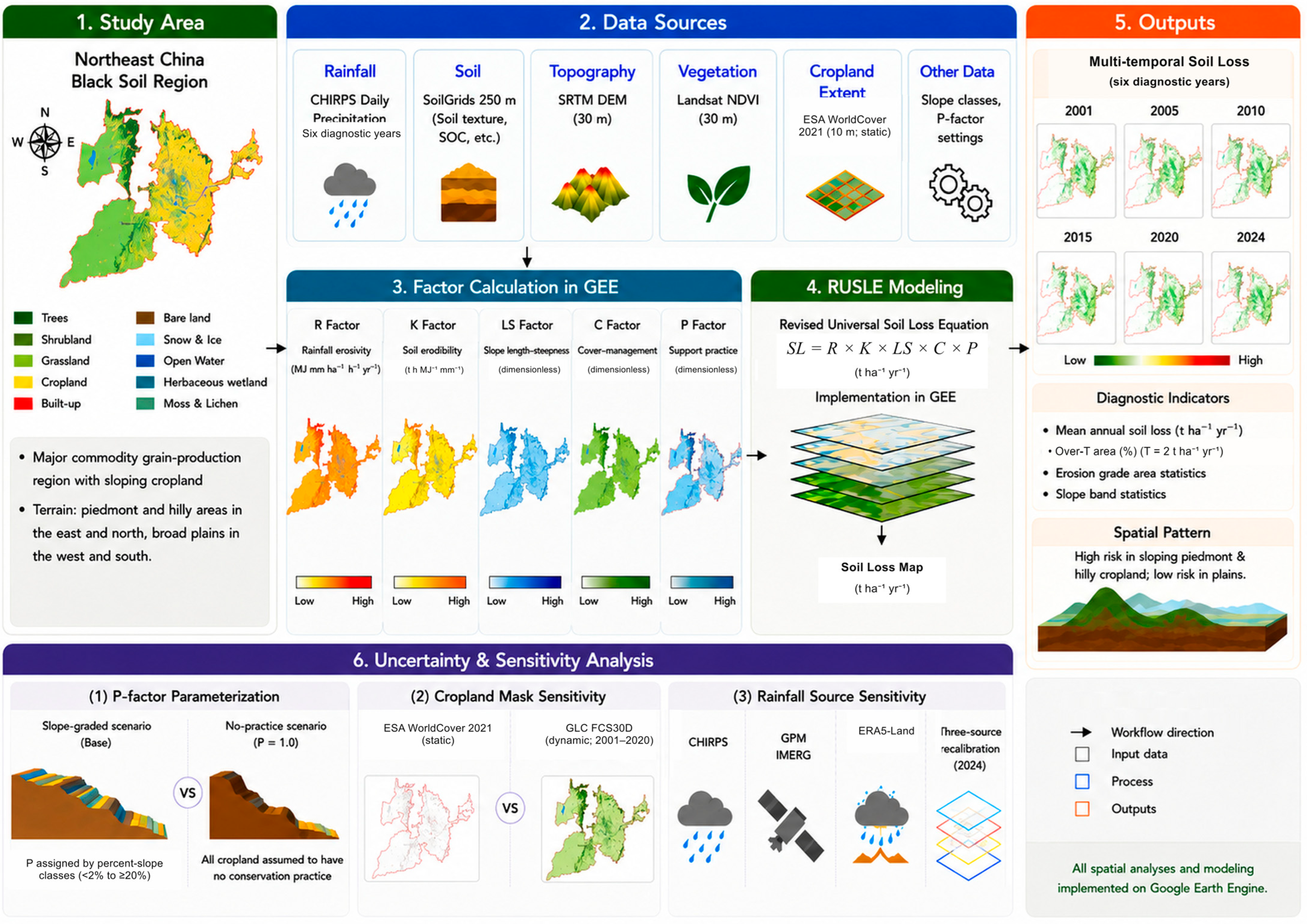
The RUSLE-GEE workflow used to parameterize model factors, organize data inputs, conduct six time-slice diagnostics, and evaluate sensitivity and uncertainty is summarized in Figure 2.

2.2. RUSLE-Based Model Framework

This study adopts the five-factor multiplicative structure of a RUSLE-based empirical framework and incorporates factor parameterizations commonly used in RUSLE and Erosion/Productivity Impact Calculator (EPIC) studies. Annual mean soil loss is expressed as follows:
USLE and RUSLE were not implemented as two separate models; this study uses a RUSLE-based empirical framework that inherits the multiplicative factor structure from the broader empirical soil-loss model family.
S L = R × K × L S × C × P
where SL is annual mean soil loss (t ha−1 yr−1); R is rainfall erosivity (MJ mm ha−1 h−1 yr−1); K is soil erodibility (t h MJ−1 mm−1); LS is the dimensionless topographic factor; C is the dimensionless cover-management factor (0–1); and P is the dimensionless support-practice factor (0–1).

2.3. Rainfall Erosivity (R) Factor

The R factor represents the erosive potential of rainfall and is the most temporally variable component of the RUSLE-based framework. In principle, R should be calculated using the EI30 rainfall erosivity index, which combines total storm kinetic energy and maximum 30 min rainfall intensity, derived from continuous rainfall records. In large-scale studies where minute-resolution rainfall observations are unavailable, however, simplified empirical equations based on daily precipitation are widely used [40]. In this study, CHIRPS Daily precipitation data [39] were used to calculate R with the daily rainfall erosivity equation compiled and validated for China by Xie et al. (2016) [40]:
In this context, EI30 denotes the rainfall erosivity index calculated from total storm kinetic energy and the maximum 30 min rainfall intensity. Because continuous high-frequency rainfall records were unavailable for the full regional 2001–2024 analysis, a daily rainfall erosivity equation was used.
R = i = 1 n α · P d a i l y , i β
where Pdaily,i is the daily precipitation on day i (mm), and n is the number of effective erosive rainfall days in a year. Daily precipitation below 12 mm was set to zero, whereas rainfall days with precipitation ≥ 12 mm were included in the R-factor calculation. Xie et al. (2016) reported the parameter form of the daily-scale rainfall erosivity model for China and discussed the difference between the 12 mm erosive-event threshold and the daily-scale threshold [40]. The 12 mm threshold used here should, therefore, be interpreted as an implementation setting rather than the optimal daily threshold recommended by Xie et al. (2016) [40]. The parameters α = 0.3937 and β = 1.7265 are consistent with the warm-season daily rainfall erosivity equation summarized and validated for China by Xie et al. (2016) [40]. During calculation, R was set to zero for winter months (November to March of the following year), as a modeling assumption for the solid-precipitation and freeze–thaw context of Northeast China, thereby reducing the risk that winter precipitation would be interpreted directly as erosive rainfall.
This treatment does not imply the absence of erosion during winter or early spring. Rather, it restricts the R factor to rainfall-driven erosivity and avoids interpreting solid precipitation as erosive rainfall. Therefore, snowmelt runoff, freeze–thaw effects, and early-spring runoff over partially thawed soils are not explicitly quantified within the present RUSLE-based framework.

2.4. Soil Erodibility (K) Factor

The K factor describes the susceptibility of soil to detachment and transport by water erosion. This study used the Erosion/Productivity Impact Calculator (EPIC) empirical equation [69], with sand, silt, clay, and soil organic carbon (SOC) contents from the SoilGrids 250 m dataset:
The direct calculation pathway was as follows. SoilGrids 250 m sand (SAN, %), silt (SIL, %), clay (CLA, %), and soil organic carbon (SOC, %) were entered into the EPIC K equation to calculate four multiplicative terms: K1, the sand correction term; K2, the silt-clay ratio term; K3, the organic-carbon adjustment term; and K4, the high-sand correction term. Sand, silt, clay, and SOC were kept constant across all time slices, so K represents a baseline soil-property factor rather than a time-varying layer.
K = 0.1317 × K 1 × K 2 × K 3 × K 4
where K1 is the sand correction term, K2 is the silt-clay ratio term, K3 is the organic-carbon adjustment term, and K4 is the high-sand correction term. The coefficient 0.1317 follows the unit-conversion treatment of the EPIC K equation in the RUSLE handbook and related reviews, converting U.S. customary units to SI units (t h MJ−1 mm−1) [25,26].
K was held constant because temporally consistent annual soil texture and SOC datasets for 2001–2024 are unavailable at the regional scale. This setting maintains cross-year comparability and isolates temporal differences mainly associated with R and C, but it should not be interpreted as evidence that field soil erodibility remained unchanged.

2.5. Topographic (LS) Factor

The LS factor represents the enhancement of erosion by terrain and is the product of the slope-length factor L and the slope-steepness factor S. Slope was derived from the SRTM 30 m DEM and resampled to the target scale during GEE processing. Slope length was set to a fixed λ = 50 m as a cross-year scenario assumption to avoid introducing additional uncertainty from large-scale flow-accumulation calculations in GEE.
L = λ 22.13 m
S = 10.8 · s i n θ + 0.03 , s < 9 % S = 16.8 · s i n θ 0.50 , s 9 %
where λ is slope length (m), fixed at 50 m in this study; m is the slope-length exponent, calculated using the continuous RUSLE expression based on the slope ratio β: β = (sinθ/0.0896)/(3·sin0.8θ + 0.56), and m = β/(1 + β), where θ is the slope angle in radians and s is percent slope, calculated as s = 100 × tanθ [25]. The S factor follows the 9% slope-segmented formulation proposed by McCool et al. (1987) and adopted in RUSLE [70], with the breakpoint s = 9% corresponding to a slope angle of approximately 5.14°.

2.6. Cover-Management (C) Factor

The C factor represents the reduction in erosion by vegetation cover. Landsat imagery [68] was used to calculate the normalized difference vegetation index (NDVI), from which fractional vegetation cover (fc) was derived. C values were then calculated using the logarithmic relationship between vegetation cover and the C factor proposed by Cai et al. (2000) [71]; similar NDVI/fc-C frameworks have also been used in RUSLE applications in the black soil region [15]. Because spatially exhaustive, year-consistent observations of crop management and surface cover are unavailable for the entire black soil region, the NDVI/fc-C empirical relationship was used as a regional remote-sensing proxy to maintain consistency and reproducibility across years. C was calculated monthly and then averaged annually using monthly R-factor weights.
f c = N D V I N D V I s o i l N D V I v e g N D V I s o i l
where NDVIsoil = 0.05 and NDVIveg = 0.80 are fixed implementation parameters used for NDVI endmember normalization. fc was constrained to the range 0–1. Where the equation tended toward extremely low C values under high-cover conditions, C = 0.001 was imposed as the numerical lower bound. These endmembers and lower bounds should be understood as model implementation assumptions. The C factor was calculated piecewise from fc as follows: (1) fc ≤ 0 (bare ground/non-growing season): C = 1.0; (2) 0 < fc < 0.783: C = 0.6508 − 0.3436 lg(fc); and (3) fc ≥ 0.783: C = 0.001. Monthly Cj was finally constrained to 0–1. Annual C was then calculated using R-factor weighting:
C a n n u a l = j = 1 12 R j R a n n × C j
where Rj is the R factor for month j, Rann is the annual total R factor, and Cj is the C value for month j. During the growing season (May–September), monthly mean Landsat NDVI composites were used to calculate fc and Cj, and missing monthly pixels were filled using the growing-season mean NDVI. During the non-growing season (October–April of the following year), Cj was set uniformly to 1.0 because the soil surface is exposed after harvest. R-weighting ensures that vegetation conditions during months with erosive rainfall make a larger contribution to annual C.

2.7. Support-Practice (P) Factor

The P factor represents the ratio of soil loss under conservation practices to soil loss under straight-slope cultivation, and ranges from 0 to 1. Because spatially explicit, year-by-year observations of actual soil and water conservation practices are unavailable for the entire black soil region, this study did not attempt to estimate the true P distribution directly. Instead, two scenarios were used to quantify the uncertainty introduced by P-factor specification:
(1)
Slope-graded P-factor scenario: cropland was divided by percent slope into six classes (<2%, 2–7%, 7–10%, 10–15%, 15–20%, and ≥20%), assigned p values of 1.00, 0.18, 0.25, 0.30, 0.40, and 0.55, respectively. This scenario, together with the no-practice scenario, defines the range of P-factor parameterization effects on SL estimates and does not represent the spatial distribution of actual conservation measures. The setting assumes strong protection on 2–7% sloping cropland (p = 0.18), with weakening protection as slope increases (P gradually increasing to 0.55), while flat cropland below 2% is treated as p = 1.0. As an external reference, Chen et al. (2024) listed cropland support-practice-factor values of 0.180, 0.352, and 0.399 in a RUSLE application for the black soil region and adopted or cited a mean cropland support-practice p value of 0.331 [15], indicating that p values below 1 have precedent in comparable studies.
(2)
No-practice upper-bound scenario (p = 1.0): all cropland was assumed to have no support-practice effects, providing a theoretical upper bound for the effect of P-factor parameterization.
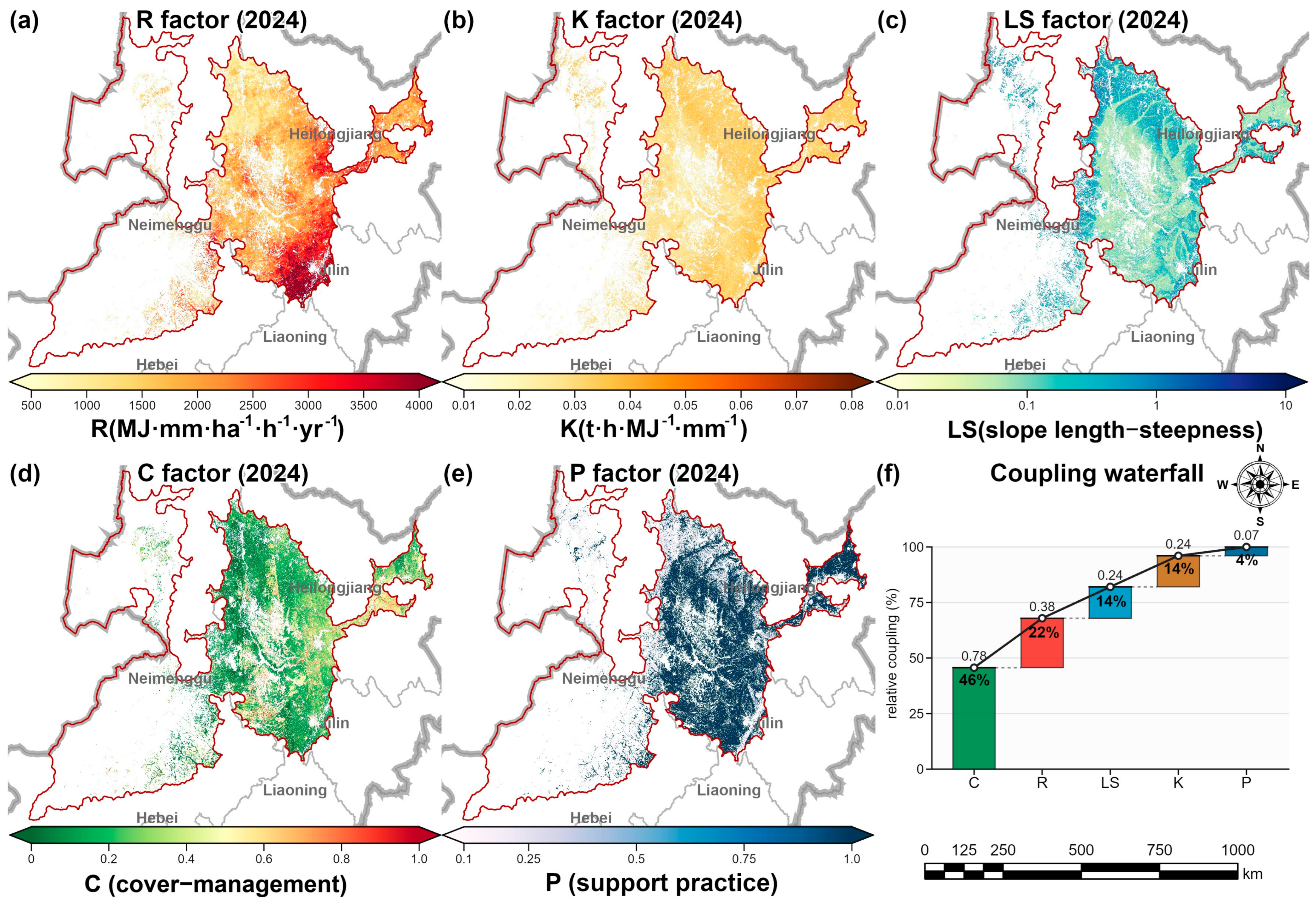
Together, these two scenarios define an uncertainty interval for P-factor parameterization. Slope units were specified as percent slope, and this choice was confirmed from USDA Agriculture Handbook No. 537 (AH-537) [24]. In AH-537, contouring p values range from 0.50 to 0.90 and serve as a reference for units and order of magnitude; however, they cannot be used to directly derive the 0.18–0.55 scenario sequence used here. The p value sequence in this study should, therefore, be understood as a model scenario assumption, requiring future verification with field surveys and spatial data on conservation measures. The spatial distribution of the five RUSLE factors in 2024 and their pixel-level coupling with SL are shown in Figure 3.

2.8. Diagnostic Indicators

A multidimensional set of diagnostic indicators was developed: (1) SLmean (t ha−1 yr−1), the arithmetic mean soil loss of cropland pixels in the study area; (2) the over-T percentage, defined as the proportion of cropland area with SL exceeding the tolerable soil loss threshold T; here T = 2 t ha−1 yr−1 was adopted according to the Chinese industry standard SL 190-2007 [72]; (3) erosion-grade area, calculated according to the six SL 190-2007 classes: very slight (<2), slight (2–25), moderate (25–50), intense (50–80), very intense (80–150), and severe (>150 t ha−1 yr−1) [72]; and (4) slope band statistics, for which cropland was divided into six slope classes (<2%, 2–7%, 7–10%, 10–15%, 15–20%, and ≥20%) and SLmean, the over-T percentage, and factor means were calculated for each band.

2.9. Sensitivity and Uncertainty Analysis

The uncertainty analysis comprised three lines of evidence. First, the P-factor slope-unit check compared SL differences under percent slope and degree-based slope settings to evaluate the bias that could arise from unit misuse; this issue was constrained using the unit description in AH-537. Second, cropland-mask sensitivity was tested by comparing the ESA WorldCover 2021 static cropland mask with the GLC FCS30D dynamic land-cover mask for 2001–2020 in an independent experiment. This test assessed the effect of cropland-mask replacement on cropland extent and SL estimates. Third, rainfall-source sensitivity was assessed using a 2024 three-source recalculation, in which CHIRPS, GPM IMERG, and the ERA5-Land reanalysis product were compared under otherwise identical settings. Except for the P-unit check, these analyses characterize the potential magnitude of input data-source substitution. The GLC mask comparison does not include 2024, and the rainfall-source sensitivity test covers only 2024; neither result should, therefore, be extrapolated as an uncertainty boundary for the full 2001–2024 period. The main results used the ESA WorldCover 2021 static cropland mask to isolate changes in R and C under a unified spatial sampling frame; dynamic cropland-mask results are reported only as a sensitivity experiment. The factor-specific temporal treatment adopted across the six diagnostic years is summarized in Table 1.
This table clarifies that R and C were recalculated for each diagnostic year, K and LS were baseline static layers, and P was a fixed slope-grade scenario rather than an observed annual conservation-practice layer.

3. Results

3.1. Multi-Temporal Soil Loss Diagnosis

Under the slope-graded P-factor scenario, the model-estimated annual mean soil loss (SLmean) showed marked variation among time slices. It was 1.85 t ha−1 yr−1 in 2001, rose to 3.07 t ha−1 yr−1 in 2005—the highest value among the six slices—declined to 2.31 t ha−1 yr−1 in 2010, reached 2.52 and 2.97 t ha−1 yr−1 in 2015 and 2020, respectively, and fell to 1.60 t ha−1 yr−1 in 2024, the lowest value. The over-T percentage varied more strongly: in 2005, 52.9% of effective cropland analysis pixels exceeded T = 2 t ha−1 yr−1, whereas the corresponding proportion in 2024 was 25.2%.
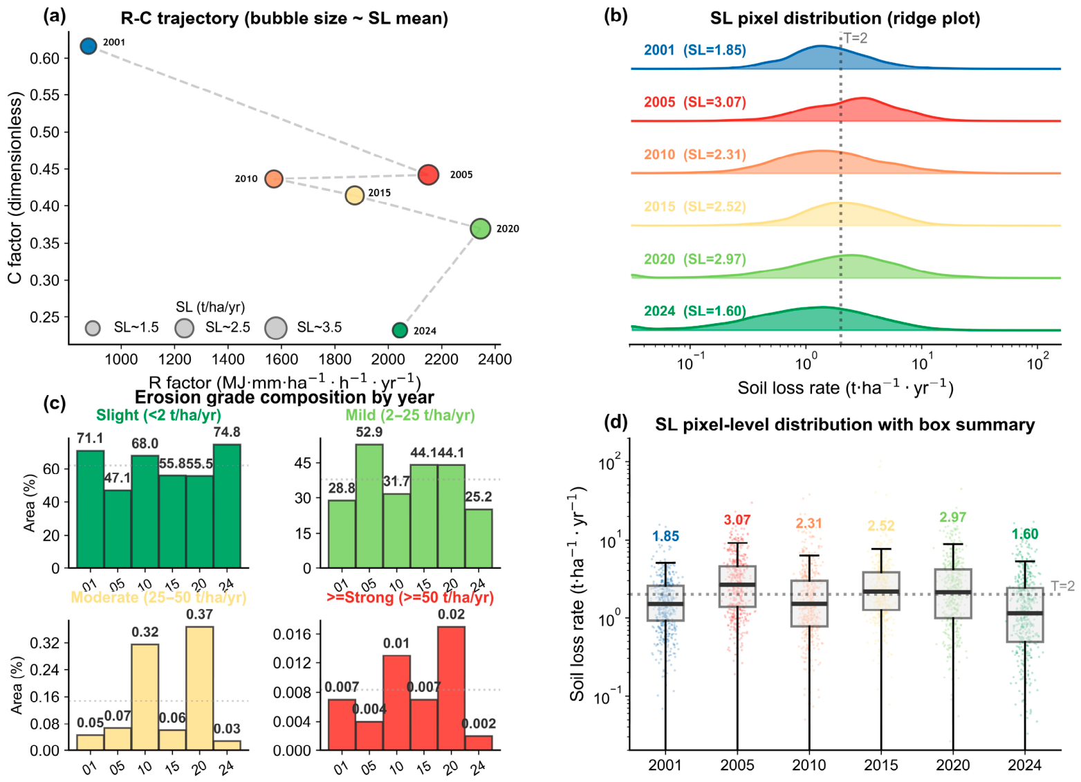
At the factor level, variation in SLmean across the six discrete time slices mainly reflected the combination of CHIRPS-derived R and Landsat-NDVI-derived C. The R factor increased from 878 MJ mm ha−1 h−1 yr−1 in 2001 to 2345 MJ mm ha−1 h−1 yr−1 in 2020, a 167% increase, while the C factor declined from 0.616 in 2001 to 0.232 in 2024, a 62% decrease. When the R × C product was high, SL tended to be high; when a low C factor offset a high R factor, SL remained low. Because K, LS, and P were kept static over time, differences in SL among the six slices mainly resulted from the R-C input combination. Given the limited number of sampled years (n = 6), the absence of regional field calibration for C, and the lack of formal trend testing, this relationship is not interpreted here as a long-term trend or causal attribution. The integrated diagnosis of R, C, SL, and erosion-grade areas for the six time slices is shown in Figure 4.
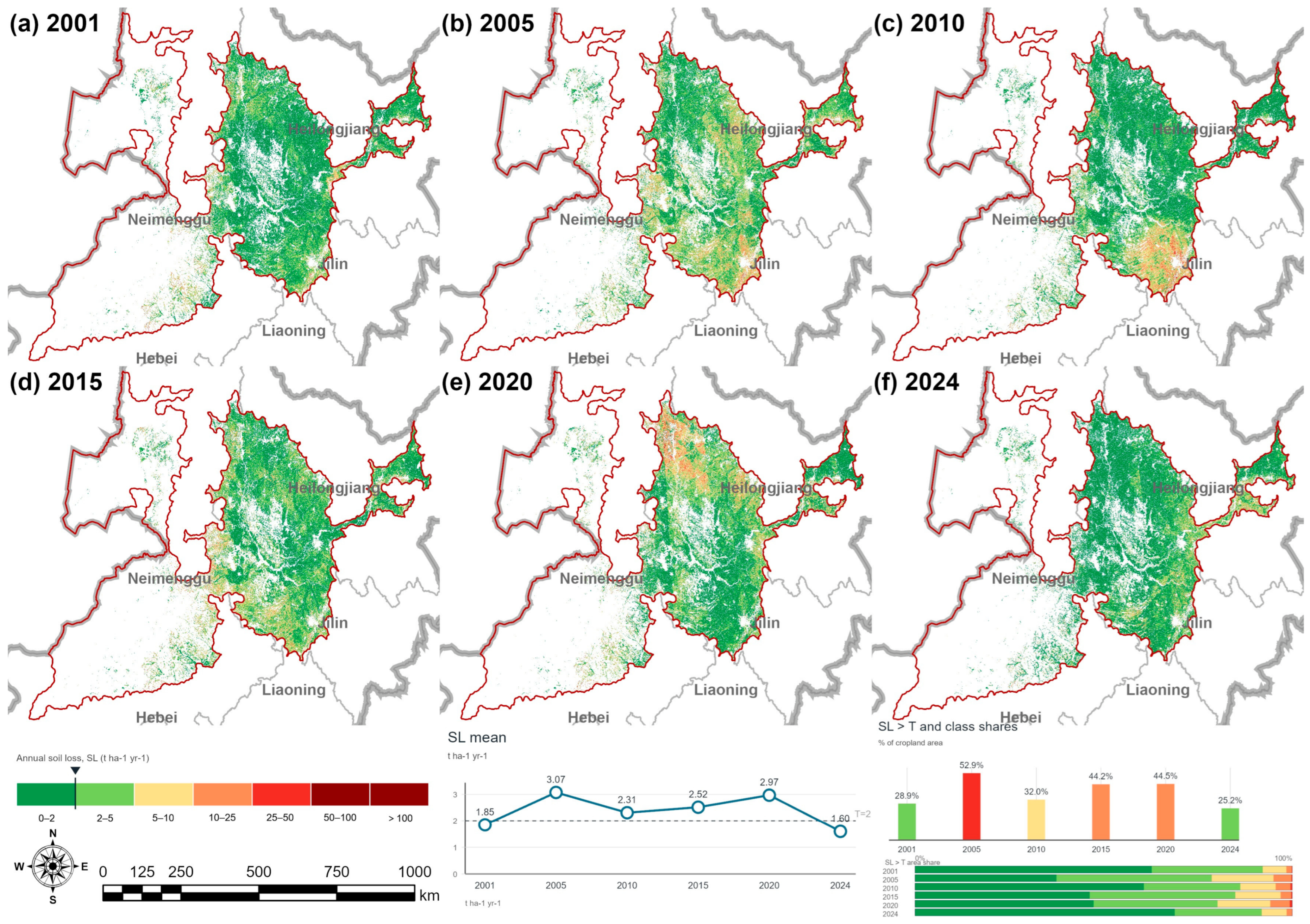
Spatially, high-SL areas were concentrated mainly in the piedmont and hilly transition zones of the Greater and Lesser Khingan Mountains and the Changbai Mountains. These areas have steeper slopes and relatively higher precipitation, so the combined effect of R and LS increased model-estimated erosion intensity. In contrast, the core cropland areas of the Songnen and Sanjiang plains are flat and have low LS values; even in years with high R, absolute SL values mostly remained within the very slight to slight erosion classes. The high SL values in 2005 and 2020 were reflected not only in higher means but also in increased 95th percentiles, indicating a stronger contribution from high-value pixels in high-rainfall years. In 2024, the 95th percentile of SL decreased to 5.47 t ha−1 yr−1. The spatial distribution of SL across the six time slices and the pattern of high- and low-value areas are shown in Figure 5.

3.2. Erosion-Grade Area Distribution

The erosion-grade structure is further shown in Figure 4 and Figure 5. Under the 2024 slope-graded P-factor scenario, 74.81% of cropland was classified as very slight erosion (<2 t ha−1 yr−1), 25.16% as slight erosion (2–25 t ha−1 yr−1), and only 0.03% as moderate or above. In 2005, when SLmean was higher, the slight-erosion share increased to 52.88%, the very slight share decreased to 47.05%, and the moderate-erosion area increased to 137 km2. Even in 2005, the strongest erosion year among the six slices, moderate-or-above erosion accounted for less than 0.1% of cropland, indicating that low-grade erosion dominated the study area.

3.3. Diagnosis Stratified by Slope Band

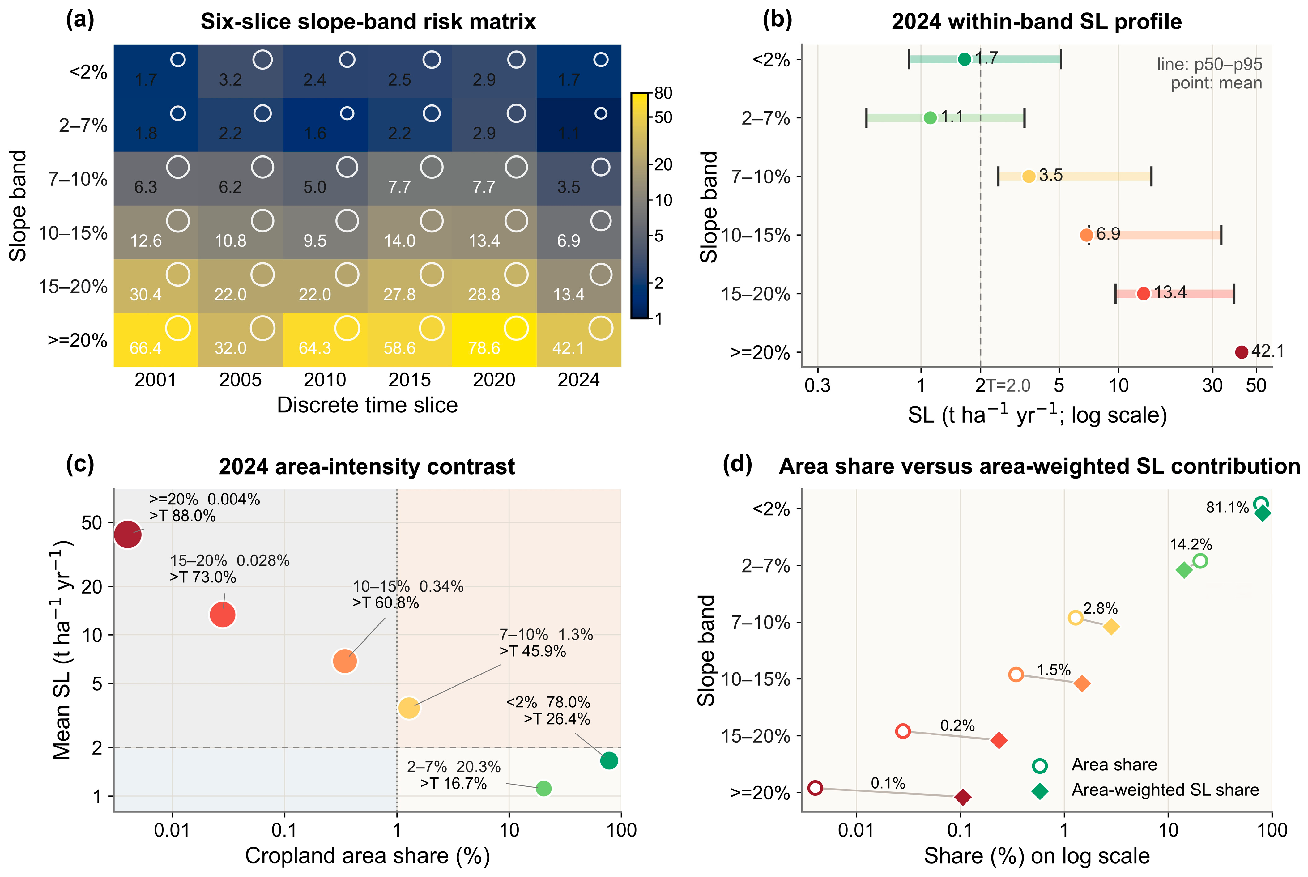
Approximately 78.0% of cropland in the study area lies in the <2% flat band, and 20.3% lies in the 2–7% gentle-slope band; together, these two classes account for 98.3% of cropland. Cropland with slopes ≥ 10% covers only about 772 km2 (0.38%), and extremely steep cropland with slopes ≥ 15% covers only 64 km2 (0.032%).
SL intensity showed clear stratification by slope band. In 2024, SLmean was 1.66 t ha−1 yr−1 in the <2% band, 1.11 in the 2–7% band, 3.52 in the 7–10% band, 6.88 in the 10–15% band, 13.39 in the 15–20% band, and 42.10 t ha−1 yr−1 in the ≥20% band. The ≥20% band had an SL value approximately 38 times that of the 2–7% band. For slope bands ≥ 2%, SLmean increased with slope. However, because p = 1.0 was assigned to the <2% band and p = 0.18 to the 2–7% band, SLmean in the <2% band was slightly higher than that in the 2–7% band in some years. This pattern reflects the mathematical effect of P-factor parameterization on low-slope classes and should not be interpreted as a direct physical erosion process.
To evaluate the effect of assigning p = 1.0 to the <2% band, a proportional recalculation was performed using the means from Figure 6 and its associated slope band statistics. If P in the <2% band were reduced to 0.18, the same as in the 2–7% band, SLmean for the <2% band would decline from 1.66 to 0.30 t ha−1 yr−1, and regional SLmean would decrease from 1.60 to 0.54 t ha−1 yr−1 (−66.3%). The rank order of SL between the <2% and 2–7% bands would also reverse. This result shows that SL ranking in low-slope bands is highly sensitive to the P setting and should not be interpreted physically outside the P-scenario assumption.
The over-T percentage was generally high in steep slope bands (≥10%), exceeding 64% in some years and even reaching 96%, markedly higher than in flat areas. However, cropland with slopes ≥ 15% covered only about 64 km2, accounting for 0.032% of total cropland, which limits the statistical generalizability of this class. The main value of the slope band diagnosis is, therefore, to reveal the structural sensitivity of the RUSLE-based framework to the LS factor, rather than to provide precise estimates of erosion intensity in high-slope areas. The six-period risk matrix, 2024 distributional structure, and area–intensity relationship by slope band are shown in Figure 6.

3.4. Uncertainty and Sensitivity Analysis

3.4.1. P-Factor Slope-Unit Check

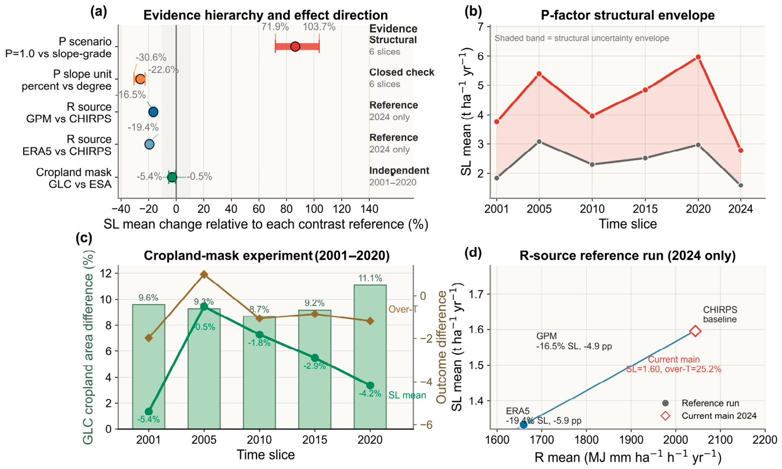
The P-factor slope-unit check evaluated the potential SL bias caused by using slope in degrees rather than percent slope. Across the six time slices, SLmean calculated with percent slope was 22.6–30.6% lower than under the degree-based slope setting, and the over-T area decreased by 12,742–20,178 km2. The difference arises because the same real slope has different numeric values under percent and degree units; for example, a 10% slope is approximately 5.7°, which can assign pixels to different P classes. Since AH-537 specifies percent slope, the main results use percent slope; degree-based slope results are retained only as a sensitivity reference for unit misuse, not as a persistent source of model uncertainty.

3.4.2. Sensitivity to Cropland Mask Data Source

Relative to ESA WorldCover 2021, the cropland area identified by GLC FCS30D in 2001–2020 was 8.7–11.1% larger, mainly because of classification differences along forest and grassland edge pixels. When propagated into SL calculation, the relative difference in SLmean was −5.4% to −0.5%, meaning that SL was slightly lower under the GLC mask. This result indicates only that, in the 2001–2020 dynamic-mask comparison experiment, replacing the mask had a smaller effect on regional SLmean than P-unit misuse and 2024 rainfall-source substitution. It does not validate the historical realism of the static ESA mask, nor does it represent dynamic cropland-mask uncertainty for 2024.

3.4.3. Sensitivity to Rainfall Data Source

In the 2024 three-source recalculation experiment, the CHIRPS Daily baseline yielded Rmean = 2043.3 MJ mm ha−1 h−1 yr−1, SLmean = 1.60 t ha−1 yr−1, and an over-T percentage of 25.2%. Using GPM IMERG precipitation, Rmean decreased to 1659.6 MJ mm ha−1 h−1 yr−1 and SLmean to 1.33 t ha−1 yr−1, a 16.53% relative reduction in SLmean. Using the ERA5-Land reanalysis product, Rmean decreased to 1592.3 MJ mm ha−1 h−1 yr−1 and SLmean to 1.29 t ha−1 yr−1, a 19.43% relative reduction. These results characterize the potential effect of rainfall-source substitution under the current 2024 convention and should not be extrapolated as the uncertainty boundary for the full study period. The same November–March filtering was applied consistently to CHIRPS, GPM IMERG, and ERA5-Land R calculations, and the resulting R factors were propagated to SL and the over-T percentage. Sensitivity results for P-factor scenarios, P-factor slope unit, cropland mask, and rainfall data source are shown in Figure 7.

4. Discussion

4.1. The Counteracting R-C Effect in Interannual SL Variation

SLmean across the six time slices fluctuated rather than followed a linear trend. Because only six discrete years were sampled, the result should be interpreted as differences among model-estimated states for selected years, not as a statistically defined long-term trend. The R factor increased from 878 MJ mm ha−1 h−1 yr−1 in 2001 to 2345 MJ mm ha−1 h−1 yr−1 in 2020 (+167%), reflecting precipitation differences captured by the CHIRPS product in these slices. The Landsat-NDVI-derived C factor declined from 0.616 to 0.232, which may reflect phenology, crop structure, management practices, and remote-sensing observation conditions. Because this study did not adopt a causal identification design, changes in R or C are not attributed to a single driver.
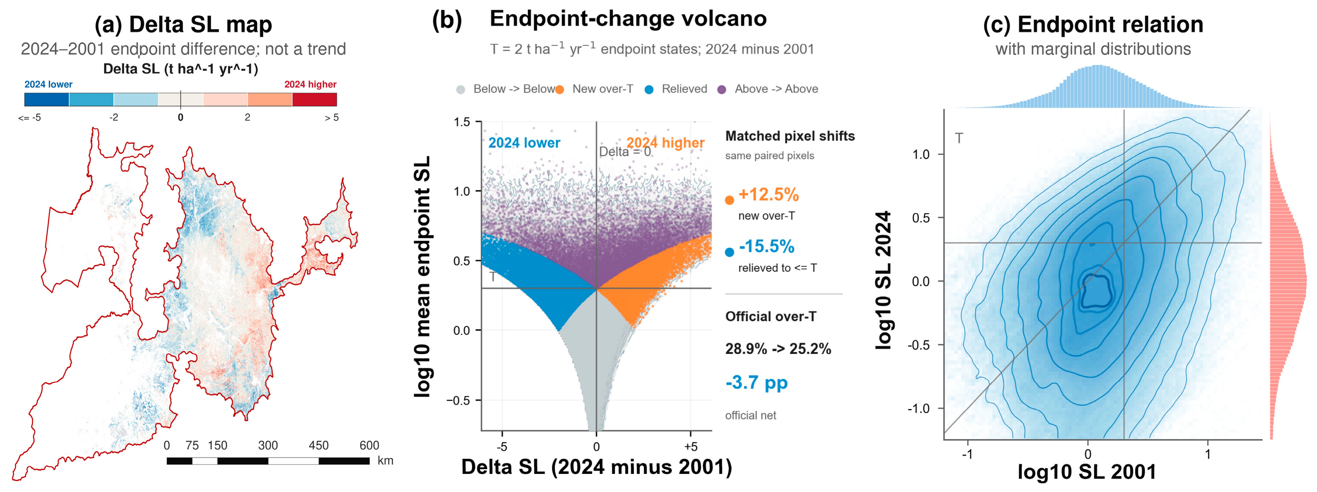
Within the RUSLE multiplicative structure, when R increases and C decreases, the direction of SL change depends on the relative magnitude of the increase in R and the decrease in C. In 2005, R increased by 145% relative to 2001, whereas the decrease in C was more limited (−28%), producing the highest SL among the six time slices (3.07 t ha−1 yr−1). In 2024, R remained high (2044 MJ mm ha−1 h−1 yr−1), but C decreased to 0.232, 48% lower than in 2005, reducing the R × C product and yielding the lowest SL (1.60 t ha−1 yr−1). Endpoint differences in SL, over-T state transitions, and the endpoint relationship between 2001 and 2024 are shown in Figure 8.
Mechanistically, this pattern is a counteracting R-C effect within the static K-LS-P background: higher rainfall erosivity increases potential soil loss, whereas lower C values reduce the effective erosive forcing before multiplication by K, LS, and P. Thus, the high-R year 2020 did not exceed the 2005 SLmean peak because C was already lower than in the early slices.
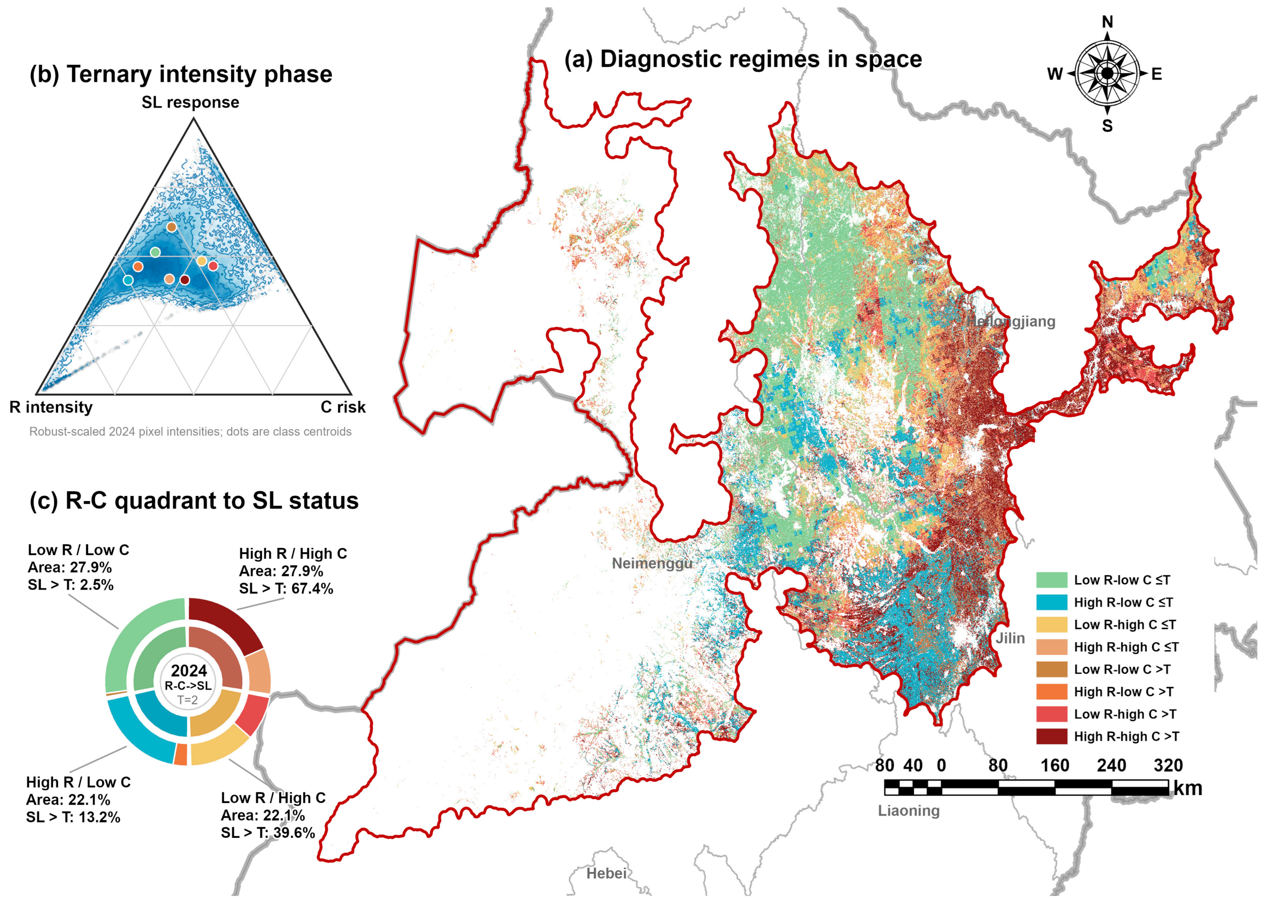
The time-slice results indicate that SL change is not governed by a single factor, but by the combined spatial and temporal effects of R and C. To avoid interpreting the low SL in 2024 solely from regional means, this study further constructed an R-C-SL ternary diagnosis. R and C were divided into high and low groups by the median of effective pixels and combined with the T = 2 t ha−1 yr−1 threshold to identify pixel states. This diagnosis addresses two questions: whether low C under high R conditions is sufficient to keep SL below T, and which R-C combinations dominate among over-T pixels. The spatial combination of R, C, and SL threshold states in 2024 is shown in Figure 9.

4.2. External Consistency Check

Because runoff-plot observations and river-sediment records are unavailable within the study area, strict model validation could not be conducted. This section, therefore, provides only a qualitative consistency check against existing RUSLE studies in the black soil region and adjacent basins [15,16]. Previous studies indicate that water erosion patterns in the black soil region are jointly controlled by slope, land use, vegetation cover, and rainfall variability, and that regional-scale estimates are highly sensitive to model inputs and parameter settings. In all years examined here, the combined share of very slight and slight erosion exceeded 99.6%, which can be viewed as a reference for spatial-pattern plausibility under the present modeling convention. This qualitative consistency should not be regarded as validation of absolute erosion rates; the results remain spatial estimates conditioned on the present model parameterization.

4.3. Comparison with Previous Studies

The SLmean values reported here differ from those in previous studies of the Hulan River Basin. Such differences cannot be compared directly without accounting for study-area extent, land-use domain, P-factor setting, LS algorithm, rainfall source, and statistical scale. Mean erosion intensity in sub-basin studies varies substantially with year, domain, and model configuration. For example, Cheng et al. reported that the Hulan River Basin mean increased from 4.63 t ha−1 yr−1 in 2001 to 7.34 t ha−1 yr−1 in 2020 [16]; Chen et al. reported a mean annual water erosion rate of 1020.16 t km−2 yr−1 in 2020 [15], equivalent to approximately 10.20 t ha−1 yr−1. Under the no-practice scenario in this study, the 2024 SLmean was 2.78 t ha−1 yr−1, clearly higher than the 1.60 t ha−1 yr−1 estimated under the slope-graded P-factor scenario. This contrast shows that P-factor parameterization alone can substantially alter the regional mean. Cross-study numerical comparisons should, therefore, first harmonize the area of interest (AOI), land-use domain, P factor, LS algorithm, and R source. This interpretation is consistent with the review by Benavidez et al. [26], which emphasizes that subfactor choices and regional calibration strongly affect RUSLE outputs.
At the spatial-pattern level, the results are consistent with previous black-soil studies that locate higher erosion risk in relief-sensitive cropland, hilly margins, and gully-prone landscapes rather than uniformly across the plains [18,20,22,23]. Methodological differences among studies should be interpreted as the combined effect of AOI definition, cropland mask, time slice, rainfall source, C-factor construction, LS algorithm, and P-factor assumptions, consistent with broader RUSLE uncertainty and harmonization literature [26,28,64].

4.4. Quantitative Bounds of Model-Input Uncertainty

The sensitivity analysis shows that RUSLE-factor input choices can substantially affect regional SL estimates. Misusing the P-factor slope unit can cause a 22.6–30.6% bias in SL, although this issue is constrained here by checking the unit specification in AH-537. Replacing the rainfall data source in the 2024 three-source recalculation produced a 16.53–19.43% difference in SLmean, mainly reflecting differences among CHIRPS, Global Precipitation Measurement Integrated Multi-satellitE Retrievals for GPM (GPM IMERG), and ECMWF Reanalysis v5 Land (ERA5-Land) in data source, retrieval mechanism, and spatial resolution; this magnitude should not be extrapolated as a general rainfall-source uncertainty for all six time slices. Cropland-mask replacement had a smaller effect in the 2001–2020 Global Land Cover with Fine Classification System at 30 m (GLC FCS30D) comparison experiment, with relative differences in SLmean ranging from −5.4% to −0.5%; however, this result does not prove that the static ESA mask fully represents historical cropland boundaries.
By contrast, the numerical specification of the P factor constitutes a more substantial structural uncertainty. Under the p = 1.0 no-practice upper-bound scenario, SLmean increased by 71.9–103.7% relative to the slope-graded P-factor scenario across the six time slices, and the over-T percentage increased by 9.0–13.4 percentage points. In 2024, SLmean rose from 1.60 to 2.78 t ha−1 yr−1 (+74.1%), and the over-T percentage increased from 25.2% to 36.1% (+10.95 percentage points). In the absence of spatial data on actual soil and water conservation practices, P-factor parameterization is, therefore, one of the main sources of uncertainty in absolute SL estimates.

4.5. Management Interpretation Boundaries of the Slope Band Diagnosis

The slope band results reveal strong spatial heterogeneity in cropland erosion risk across the black soil region of Northeast China. Although 78% of cropland lies in the <2% flat band, its large area means that total erosion contribution in high-rainfall years cannot be ignored. At the same time, SL estimates for flat cropland are highly sensitive to the p = 1.0 setting; if conservation practices are present in reality, actual SL could be substantially lower than estimated here. Results for flat cropland are, therefore, better used as clues for field surveys of management practices than as direct evidence for intervention prioritization.
Cropland with slopes ≥ 7% accounts for approximately 1.7% of the total area (about 3400 km2), yet its SL intensity is clearly higher than that of flat areas; in 2024, the over-T percentage exceeded 70% for the small amount of cropland steeper than 15%. Because steep cropland occupies a limited area and because observed conservation-measure distributions and external validation data are lacking, slope band results should be interpreted as a diagnosis of the structural sensitivity of RUSLE to the LS factor. These areas can serve as candidate zones for subsequent high-resolution model validation, conservation-practice surveys, and field verification.
Management implications should, therefore, be framed cautiously. The maps and slope band diagnostics identify relative erosion-risk patterns and candidate areas for follow-up investigation, but site-specific conservation engineering requires field validation, observed conservation-practice information, and local runoff or sediment evidence.

4.6. Study Limitations

The conclusions of this study should be interpreted within the applicable domain of an empirical RUSLE model driven by multi-source remote-sensing inputs. First, to ensure comparability among the 2001–2024 time slices, a unified parameterization scheme was adopted for the LS, C, and P factors. This scheme included fixed slope length, NDVI endmembers, monthly R weighting, and slope-graded P-factor values. These settings support a consistent regional diagnostic convention, but they are not direct observations of true pixel-level flow length, crop management, or engineering measures. Second, the R, K, and C factors rely, respectively, on CHIRPS precipitation, SoilGrids soil properties, and Landsat vegetation indices. The results may, therefore, be affected by spatial resolution, cross-sensor consistency, and the static representation of soil properties. Rainfall-source, cropland-mask, and P-factor scenarios were used to bound major input uncertainties, but local intense rainfall, field-scale management practices, and long-term soil-property change require further testing with higher-resolution data. Third, this study selected six representative time slices for diagnosis; the results should be interpreted as differences among discrete model-estimated states rather than as a continuous time-series trend.
The static K assumption is a structural limitation because SOC, texture, and management effects may change soil erodibility over time. In addition, snowmelt- and freeze–thaw-driven erosion in late winter and early spring is outside the rainfall-driven RUSLE parameterization and may be underrepresented, especially on sloping cropland and hilly margins.

5. Conclusions

Using a RUSLE-based model and GEE, this study diagnosed water erosion intensity on cropland across six time slices from 2001 to 2024 in the black soil region of Northeast China and evaluated associated sensitivity and uncertainty. The main conclusions are as follows:
(1)
Under the slope-graded P-factor scenario, regional SLmean ranged from 1.60 to 3.07 t ha−1 yr−1 across the six time slices, showing fluctuation among discrete years rather than a linear trend. The years 2005 and 2020 had relatively high SL values, whereas 2024 had the lowest value. This variation mainly reflected the combined behavior of CHIRPS-derived R and Landsat-NDVI-derived C under the current model setting.
(2)
The proportion of cropland exceeding the tolerable soil loss threshold, T = 2 t ha−1 yr−1, ranged from 25.2% to 52.9%. The overall erosion-grade structure was dominated by very slight and slight erosion, which together accounted for more than 99.6% of cropland. Nevertheless, the over-T percentage was sensitive to the R-C input combination and P-factor parameterization in the selected years, with rainfall erosivity being an important component.
(3)
The P factor is the most important structural source of uncertainty in the present model. Relative to the slope-graded P-factor scenario, the no-practice upper-bound scenario increased SLmean by 71.9–103.7% and the over-T percentage by 9.0–13.4 percentage points across the six slices. Misusing slope degrees rather than percent slope in the P-factor lookup can cause a 22.6–30.6% bias in SL, but the original AH-537 text confirms the use of percent slope. Rainfall-source substitution in the 2024 three-source recalculation produced a potential effect of 16.53–19.43%, whereas replacing the ESA mask with the GLC dynamic cropland mask for 2001–2020 produced SLmean differences of 0.5–5.4%.
(4)
Slope band stratification reveals the structural sensitivity of RUSLE to terrain. Although 98.3% of cropland lies in the <7% gentle-slope bands, cropland with slopes ≥ 10% had SL intensity 6–38 times higher than that of gentle slopes. Because high-slope cropland occupied a very small area (only 64 km2 for slopes ≥ 15%), conclusions for these classes have limited statistical generalizability.
In summary, this study developed a multi-temporal RUSLE remote-sensing diagnostic framework under harmonized inputs and a unified black soil region boundary, quantitatively revealing spatiotemporal fluctuations in water erosion on cropland, the structural sensitivity of slope bands, and uncertainty bounds associated with the P factor, rainfall source, and cropland mask. The results provide spatial evidence for subsequent field verification, conservation-practice surveys, and high-resolution model validation. Because runoff-plot or sediment-observation validation was unavailable, the results should be combined with field verification before being used for intervention prioritization or engineering planning.
Overall, the scientific contribution is a reproducible RUSLE-GEE diagnostic workflow that separates relative spatial erosion patterns from key structural uncertainties, especially P-factor specification, rainfall-source choice, cropland-mask choice, static K representation, and the exclusion of snowmelt/freeze–thaw erosion processes.

Author Contributions

Conceptualization, D.S. and K.X.; methodology, D.S., C.H. and D.C.; software, D.S. and X.L.; validation, T.F., Q.M. and Y.Z.; formal analysis, D.S.; investigation, D.S., B.P., Y.Z., T.Z. and B.Z.; resources, Y.L. and T.F.; data curation, D.S. and J.L.; writing—original draft preparation, D.S.; writing—review and editing, J.X., T.F. and H.W.; visualisation, D.S.; supervision, K.X.; project administration, K.X.; funding acquisition, K.X. All authors have read and agreed to the published version of the manuscript.

Funding

This research was funded by the Guangxi Philosophy and Social Sciences Research (No. ZX02080032225001).

Institutional Review Board Statement

Not applicable.

Informed Consent Statement

Not applicable.

Data Availability Statement

The datasets employed in this study—including CHIRPS Daily, SoilGrids 250 m, SRTM DEM, Landsat Collection 2 Level-2, ESA WorldCover 2021, GPM IMERG V07, ERA5-Land, and GLC FCS30D—are all publicly available datasets accessible through their respective data release platforms.

Conflicts of Interest

The authors declare no conflicts of interest.

References

  1. Borrelli, P.; Robinson, D.A.; Fleischer, L.R.; Lugato, E.; Ballabio, C.; Alewell, C.; Meusburger, K.; Modugno, S.; Schütt, B.; Ferro, V.; et al. An Assessment of the Global Impact of 21st Century Land Use Change on Soil Erosion. Nat. Commun. 2017, 8, 2013. [Google Scholar] [CrossRef] [Scilit] [PubMed]
  2. Panagos, P.; Borrelli, P.; Poesen, J.; Ballabio, C.; Lugato, E.; Meusburger, K.; Montanarella, L.; Alewell, C. The New Assessment of Soil Loss by Water Erosion in Europe. Environ. Sci. Policy 2015, 54, 438–447. [Google Scholar] [CrossRef] [Scilit]
  3. Pimentel, D.; Burgess, M. Soil Erosion Threatens Food Production. Agriculture 2013, 3, 443–463. [Google Scholar] [CrossRef] [Scilit]
  4. Montgomery, D.R. Soil Erosion and Agricultural Sustainability. Proc. Natl. Acad. Sci. USA 2007, 104, 13268–13272. [Google Scholar] [CrossRef] [Scilit] [PubMed]
  5. Ma, X.; Zhao, C.; Zhu, J. Aggravated Risk of Soil Erosion with Global Warming—A Global Meta-Analysis. CATENA 2021, 200, 105129. [Google Scholar] [CrossRef] [Scilit]
  6. Panagos, P.; Borrelli, P.; Matthews, F.; Liakos, L.; Bezak, N.; Diodato, N.; Ballabio, C. Global Rainfall Erosivity Projections for 2050 and 2070. J. Hydrol. 2022, 610, 127865. [Google Scholar] [CrossRef] [Scilit]
  7. Xiong, M.; Leng, G. Global Soil Water Erosion Responses to Climate and Land Use Changes. CATENA 2024, 241, 108043. [Google Scholar] [CrossRef] [Scilit]
  8. Sonderegger, T.; Pfister, S. Global Assessment of Agricultural Productivity Losses from Soil Compaction and Water Erosion. Environ. Sci. Technol. 2021, 55, 12162–12171. [Google Scholar] [CrossRef] [Scilit] [PubMed]
  9. Alewell, C.; Ringeval, B.; Ballabio, C.; Robinson, D.A.; Panagos, P.; Borrelli, P. Global Phosphorus Shortage Will Be Aggravated by Soil Erosion. Nat. Commun. 2020, 11, 4546. [Google Scholar] [CrossRef] [Scilit] [PubMed]
  10. Wang, L.; Zhou, Z.; Chen, Y.; Zeng, L.; Dai, L. How Does Digital Inclusive Finance Policy Affect the Carbon Emission Intensity of Industrial Land in the Yangtze River Economic Belt of China? Evidence from Intermediary and Threshold Effects. Land 2024, 13, 1127. [Google Scholar] [CrossRef] [Scilit]
  11. Li, G.; Zhao, X.; Jiang, Y.; Zou, Y.; Liu, S.; Li, X.; Zeng, L. How Can Digital Economy Accessibility Accelerate Urban Land Green Transformation in China? Evidence from Threshold and Intermediary Effects. Land 2025, 14, 322. [Google Scholar] [CrossRef] [Scilit]
  12. Zou, Y.; Li, X.; Zhao, X.; Yu, Z.; Hu, X.; Wang, H.; Luo, Y.; Zheng, Y.; Li, Y.; Zeng, L. Impact of Farmland Use Transition on Grain Carbon Sink Transfer in Karst Mountainous Areas. Land 2025, 14, 1734. [Google Scholar] [CrossRef] [Scilit]
  13. Yang, L.; Liang, Z.; Yao, W.; Zhu, H.; Zeng, L.; Zhao, Z. What Are the Impacts of Urbanisation on Carbon Emissions Efficiency? Evidence from Western China. Land 2023, 12, 1707. [Google Scholar] [CrossRef] [Scilit]
  14. Yuan, X.; Nie, Y.; Zeng, L.; Lu, C.; Yang, T. Exploring the Impacts of Urbanization on Eco-Efficiency in China. Land 2023, 12, 687. [Google Scholar] [CrossRef] [Scilit]
  15. Chen, C.; Yang, Z.; Liu, K.; Dai, H. Spatio-Temporal Variations of Black Soil Erosion under the Scenario of Soil Organic Carbon Change Based on RUSLE and Random Forest. Front. Environ. Sci. 2024, 12, 1455737. [Google Scholar] [CrossRef] [Scilit]
  16. Cheng, J.; Zhang, X.; Jia, M.; Su, Q.; Kong, D.; Zhang, Y. Integrated Use of GIS and USLE Models for LULC Change Analysis and Soil Erosion Risk Assessment in the Hulan River Basin, Northeastern China. Water 2024, 16, 241. [Google Scholar] [CrossRef] [Scilit]
  17. Liu, B.Y.; Zhang, G.L.; Xie, Y.; Shen, B.; Gu, Z.J.; Ding, Y.Y. Boundary Dataset of Black and Typical Black Soil Regions in Northeast China. Digit. J. Glob. Change Data Repos. 2021. [Google Scholar] [CrossRef] [Scilit]
  18. Qi, L.; Shi, P.; Dvorakova, K.; Van Oost, K.; Sun, Q.; Yu, H.; Van Wesemael, B. Detection of Soil Erosion Hotspots in the Croplands of a Typical Black Soil Region in Northeast China: Insights from Sentinel-2 Multispectral Remote Sensing. Remote Sens. 2023, 15, 1402. [Google Scholar] [CrossRef] [Scilit]
  19. Zhang, J.; Wang, M.; Liu, K.; Zhao, Z. Dynamic Changes in Soil Erosion and Challenges to Grain Productivity in the Black Soil Region of Northeast China. Ecol. Indic. 2025, 171, 113145. [Google Scholar] [CrossRef] [Scilit]
  20. Sun, L.; Zhang, S.; Tang, W.; Jamshidi, A.H.; Xu, L.; Wang, Y.; Fan, Z.; Liu, X.; Gao, L. Mechanisms and Key Driving Factors of Erosion-Induced Degradation of Sloping Cropland in the Typical Black Soil Region in Northeast China. Soil Tillage Res. 2026, 258, 107037. [Google Scholar] [CrossRef] [Scilit]
  21. Duan, X.; Xie, Y.; Ou, T.; Lu, H. Effects of Soil Erosion on Long-Term Soil Productivity in the Black Soil Region of Northeastern China. CATENA 2011, 87, 268–275. [Google Scholar] [CrossRef] [Scilit]
  22. Tang, J.; Xie, Y.; Cheng, H.; Liu, G. Impact of Farmland Landscape Characteristics on Gully Erosion in the Black Soil Region of Northeast China. CATENA 2025, 249, 108623. [Google Scholar] [CrossRef] [Scilit]
  23. Wang, H.; Yang, S.; Wang, Y.; Gu, Z.; Xiong, S.; Huang, X.; Sun, M.; Zhang, S.; Guo, L.; Cui, J.; et al. Rates and Causes of Black Soil Erosion in Northeast China. CATENA 2022, 214, 106250. [Google Scholar] [CrossRef] [Scilit]
  24. Wischmeier, W.H.; Smith, D.D. Predicting Rainfall Erosion Losses: A Guide to Conservation Planning; Agriculture Handbook No. 537; U.S. Department of Agriculture: Washington, DC, USA, 1978; 58p.
  25. Renard, K.G.; Foster, G.R.; Weesies, G.A.; McCool, D.K.; Yoder, D.C. Predicting Soil Erosion by Water: A Guide to Conservation Planning with the Revised Universal Soil Loss Equation (RUSLE); Agriculture Handbook No. 703; U.S. Department of Agriculture: Washington, DC, USA, 1997; 404p.
  26. Benavidez, R.; Jackson, B.; Maxwell, D.; Norton, K. A Review of the (Revised) Universal Soil Loss Equation ((R)USLE): With a View to Increasing Its Global Applicability and Improving Soil Loss Estimates. Hydrol. Earth Syst. Sci. 2018, 22, 6059–6086. [Google Scholar] [CrossRef] [Scilit]
  27. Parsons, A.J. How Reliable Are Our Methods for Estimating Soil Erosion by Water? Sci. Total Environ. 2019, 676, 215–221. [Google Scholar] [CrossRef] [Scilit] [PubMed]
  28. Borrelli, P.; Alewell, C.; Alvarez, P.; Anache, J.A.A.; Baartman, J.; Ballabio, C.; Bezak, N.; Biddoccu, M.; Cerdà, A.; Chalise, D.; et al. Soil Erosion Modelling: A Global Review and Statistical Analysis. Sci. Total Environ. 2021, 780, 146494. [Google Scholar] [CrossRef] [Scilit] [PubMed]
  29. Parsons, A.J.; Wainwright, J.; Mark Powell, D.; Kaduk, J.; Brazier, R.E. A Conceptual Model for Determining Soil Erosion by Water. Earth Surf. Process. Landf. 2004, 29, 1293–1302. [Google Scholar] [CrossRef] [Scilit]
  30. Panagos, P.; Borrelli, P.; Meusburger, K. A New European Slope Length and Steepness Factor (LS-Factor) for Modeling Soil Erosion by Water. Geosciences 2015, 5, 117–126. [Google Scholar] [CrossRef] [Scilit]
  31. Qin, W.; Guo, Q.; Cao, W.; Yin, Z.; Yan, Q.; Shan, Z.; Zheng, F. A New RUSLE Slope Length Factor and Its Application to Soil Erosion Assessment in a Loess Plateau Watershed. Soil Tillage Res. 2018, 182, 10–24. [Google Scholar] [CrossRef] [Scilit]
  32. Lu, S.; Liu, B.; Hu, Y.; Fu, S.; Cao, Q.; Shi, Y.; Huang, T. Soil Erosion Topographic Factor (LS): Accuracy Calculated from Different Data Sources. CATENA 2020, 187, 104334. [Google Scholar] [CrossRef] [Scilit]
  33. Yang, M.; Yang, Q.; Zhang, K.; Pang, G.; Huang, C. Global Soil Erodibility Factor (K) Mapping and Algorithm Applicability Analysis. CATENA 2024, 239, 107943. [Google Scholar] [CrossRef] [Scilit]
  34. Sun, L.; Liu, F.; Zhu, X.; Zhang, G. High-Resolution Digital Mapping of Soil Erodibility in China. Geoderma 2024, 444, 116853. [Google Scholar] [CrossRef] [Scilit]
  35. Wang, G.; Gertner, G.; Liu, X.; Anderson, A. Uncertainty Assessment of Soil Erodibility Factor for Revised Universal Soil Loss Equation. CATENA 2001, 46, 1–14. [Google Scholar] [CrossRef] [Scilit]
  36. Panagos, P.; Borrelli, P.; Meusburger, K.; Alewell, C.; Lugato, E.; Montanarella, L. Estimating the Soil Erosion Cover-Management Factor at the European Scale. Land Use Policy 2015, 48, 38–50. [Google Scholar] [CrossRef] [Scilit]
  37. Xiong, M.; Leng, G.; Tang, Q. Global Analysis of the Cover-Management Factor for Soil Erosion Modeling. Remote Sens. 2023, 15, 2868. [Google Scholar] [CrossRef] [Scilit]
  38. Schmidt, S.; Alewell, C.; Meusburger, K. Mapping Spatio-Temporal Dynamics of the Cover and Management Factor (C-Factor) for Grasslands in Switzerland. Remote Sens. Environ. 2018, 211, 89–104. [Google Scholar] [CrossRef] [Scilit]
  39. Funk, C.; Peterson, P.; Landsfeld, M.; Pedreros, D.; Verdin, J.; Shukla, S.; Husak, G.; Rowland, J.; Harrison, L.; Hoell, A.; et al. The Climate Hazards Infrared Precipitation with Stations—A New Environmental Record for Monitoring Extremes. Sci. Data 2015, 2, 150066. [Google Scholar] [CrossRef] [Scilit] [PubMed]
  40. Xie, Y.; Yin, S.; Liu, B.; Nearing, M.A.; Zhao, Y. Models for Estimating Daily Rainfall Erosivity in China. J. Hydrol. 2016, 535, 547–558. [Google Scholar] [CrossRef] [Scilit]
  41. Das, S.; Jain, M.K.; Gupta, V. A Step towards Mapping Rainfall Erosivity for India Using High-Resolution GPM Satellite Rainfall Products. CATENA 2022, 212, 106067. [Google Scholar] [CrossRef] [Scilit]
  42. Emberson, R.A. Dynamic Rainfall Erosivity Estimates Derived from IMERG Data. Hydrol. Earth Syst. Sci. 2023, 27, 3547–3563. [Google Scholar] [CrossRef] [Scilit]
  43. Wang, W.; Jiang, Y.; Yu, B.; Zhang, X.; Xie, Y.; Yin, B. Evaluation of GPM IMERG-FR Product for Computing Rainfall Erosivity for Mainland China. Remote Sens. 2024, 16, 1186. [Google Scholar] [CrossRef] [Scilit]
  44. Beguería, S.; Serrano-Notivoli, R.; Tomas-Burguera, M. Computation of Rainfall Erosivity from Daily Precipitation Amounts. Sci. Total Environ. 2018, 637–638, 359–373. [Google Scholar] [CrossRef] [Scilit] [PubMed]
  45. Panagos, P.; Borrelli, P.; Meusburger, K.; Yu, B.; Klik, A.; Jae Lim, K.; Yang, J.E.; Ni, J.; Miao, C.; Chattopadhyay, N.; et al. Global Rainfall Erosivity Assessment Based on High-Temporal Resolution Rainfall Records. Sci. Rep. 2017, 7, 4175. [Google Scholar] [CrossRef] [Scilit] [PubMed]
  46. Ballabio, C.; Borrelli, P.; Spinoni, J.; Meusburger, K.; Michaelides, S.; Beguería, S.; Klik, A.; Petan, S.; Janeček, M.; Olsen, P.; et al. Mapping Monthly Rainfall Erosivity in Europe. Sci. Total Environ. 2017, 579, 1298–1315. [Google Scholar] [CrossRef] [Scilit] [PubMed]
  47. Chen, Y.; Xu, M.; Wang, Z.; Chen, W.; Lai, C. Reexamination of the Xie Model and Spatiotemporal Variability in Rainfall Erosivity in Mainland China from 1960 to 2018. CATENA 2020, 195, 104837. [Google Scholar] [CrossRef] [Scilit]
  48. Almagro, A.; Thomé, T.C.; Colman, C.B.; Pereira, R.B.; Marcato Junior, J.; Rodrigues, D.B.B.; Oliveira, P.T.S. Improving Cover and Management Factor (C-Factor) Estimation Using Remote Sensing Approaches for Tropical Regions. Int. Soil Water Conserv. Res. 2019, 7, 325–334. [Google Scholar] [CrossRef] [Scilit]
  49. Latella, M.; Santini, M.; Balzarolo, M. On the Calculation of the Land Cover and Management Factor in Soil Erosion Assessments. CATENA 2026, 271, 110207. [Google Scholar] [CrossRef] [Scilit]
  50. Ayalew, D.A.; Deumlich, D.; Šarapatka, B.; Doktor, D. Quantifying the Sensitivity of NDVI-Based C Factor Estimation and Potential Soil Erosion Prediction Using Spaceborne Earth Observation Data. Remote Sens. 2020, 12, 1136. [Google Scholar] [CrossRef] [Scilit]
  51. Ebabu, K.; Tsunekawa, A.; Haregeweyn, N.; Tsubo, M.; Adgo, E.; Fenta, A.A.; Meshesha, D.T.; Berihun, M.L.; Sultan, D.; Vanmaercke, M.; et al. Global Analysis of Cover Management and Support Practice Factors That Control Soil Erosion and Conservation. Int. Soil Water Conserv. Res. 2022, 10, 161–176. [Google Scholar] [CrossRef] [Scilit]
  52. Panagos, P.; Borrelli, P.; Meusburger, K.; Van Der Zanden, E.H.; Poesen, J.; Alewell, C. Modelling the Effect of Support Practices (P-Factor) on the Reduction of Soil Erosion by Water at European Scale. Environ. Sci. Policy 2015, 51, 23–34. [Google Scholar] [CrossRef] [Scilit]
  53. Tian, P.; Zhu, Z.; Yue, Q.; He, Y.; Zhang, Z.; Hao, F.; Guo, W.; Chen, L.; Liu, M. Soil Erosion Assessment by RUSLE with Improved P Factor and Its Validation: Case Study on Mountainous and Hilly Areas of Hubei Province, China. Int. Soil Water Conserv. Res. 2021, 9, 433–444. [Google Scholar] [CrossRef] [Scilit]
  54. Xiong, M.; Sun, R.; Chen, L. Effects of Soil Conservation Techniques on Water Erosion Control: A Global Analysis. Sci. Total Environ. 2018, 645, 753–760. [Google Scholar] [CrossRef] [Scilit] [PubMed]
  55. Gorelick, N.; Hancher, M.; Dixon, M.; Ilyushchenko, S.; Thau, D.; Moore, R. Google Earth Engine: Planetary-Scale Geospatial Analysis for Everyone. Remote Sens. Environ. 2017, 202, 18–27. [Google Scholar] [CrossRef] [Scilit]
  56. Venter, Z.S.; Barton, D.N.; Chakraborty, T.; Simensen, T.; Singh, G. Global 10 m Land Use Land Cover Datasets: A Comparison of Dynamic World, World Cover and Esri Land Cover. Remote Sens. 2022, 14, 4101. [Google Scholar] [CrossRef] [Scilit]
  57. Tamiminia, H.; Salehi, B.; Mahdianpari, M.; Quackenbush, L.; Adeli, S.; Brisco, B. Google Earth Engine for Geo-Big Data Applications: A Meta-Analysis and Systematic Review. ISPRS J. Photogramm. Remote Sens. 2020, 164, 152–170. [Google Scholar] [CrossRef] [Scilit]
  58. Phalke, A.R.; Özdoğan, M. Large Area Cropland Extent Mapping with Landsat Data and a Generalized Classifier. Remote Sens. Environ. 2018, 219, 180–195. [Google Scholar] [CrossRef] [Scilit]
  59. Zhang, Y.-G.; Nearing, M.A.; Zhang, X.-C.; Xie, Y.; Wei, H. Projected Rainfall Erosivity Changes under Climate Change from Multimodel and Multiscenario Projections in Northeast China. J. Hydrol. 2010, 384, 97–106. [Google Scholar] [CrossRef] [Scilit]
  60. Wang, W.; Yin, S.; He, Z.; Chen, D.; Wang, H.; Klik, A. Projections of Rainfall Erosivity in Climate Change Scenarios for Mainland China. CATENA 2023, 232, 107391. [Google Scholar] [CrossRef] [Scilit]
  61. Xu, E.; Zhang, H. Change Pathway and Intersection of Rainfall, Soil, and Land Use Influencing Water-Related Soil Erosion. Ecol. Indic. 2020, 113, 106281. [Google Scholar] [CrossRef] [Scilit]
  62. Wang, Z.; Zeng, Y.; Li, C.; Yan, H.; Yu, S.; Wang, L.; Shi, Z. Telecoupling Cropland Soil Erosion with Distant Drivers within China. J. Environ. Manag. 2021, 288, 112395. [Google Scholar] [CrossRef] [Scilit] [PubMed]
  63. Ge, L.; Zheng, H.; Fu, Z.; Cai, C.; Wei, Y. Uncovering Interactive Impacts of Climate Extremes and Land Use Change on Soil Erosion Using a Coupled RUSLE-OPGD Framework. CATENA 2025, 261, 109507. [Google Scholar] [CrossRef] [Scilit]
  64. Bosco, C.; De Rigo, D.; Dewitte, O.; Poesen, J.; Panagos, P. Modelling Soil Erosion at European Scale: Towards Harmonization and Reproducibility. Nat. Hazards Earth Syst. Sci. 2015, 15, 225–245. [Google Scholar] [CrossRef] [Scilit]
  65. Li, P.; Zang, Y.; Ma, D.; Yao, W.; Holden, J.; Irvine, B.; Zhao, G. Soil Erosion Rates Assessed by RUSLE and PESERA for a Chinese Loess Plateau Catchment under Land-Cover Changes. Earth Surf. Process. Landf. 2020, 45, 707–722. [Google Scholar] [CrossRef] [Scilit]
  66. Panagos, P.; Ballabio, C.; Borrelli, P.; Meusburger, K.; Klik, A.; Rousseva, S.; Tadić, M.P.; Michaelides, S.; Hrabalíková, M.; Olsen, P.; et al. Rainfall Erosivity in Europe. Sci. Total Environ. 2015, 511, 801–814. [Google Scholar] [CrossRef] [Scilit]
  67. Farr, T.G.; Rosen, P.A.; Caro, E.; Crippen, R.; Duren, R.; Hensley, S.; Kobrick, M.; Paller, M.; Rodriguez, E.; Roth, L.; et al. The Shuttle Radar Topography Mission. Rev. Geophys. 2007, 45, RG2004. [Google Scholar] [CrossRef] [Scilit]
  68. Wulder, M.A.; Roy, D.P.; Radeloff, V.C.; Loveland, T.R.; Anderson, M.C.; Johnson, D.M.; Healey, S.; Zhu, Z.; Scambos, T.A.; Pahlevan, N.; et al. Fifty Years of Landsat Science and Impacts. Remote Sens. Environ. 2022, 280, 113195. [Google Scholar] [CrossRef] [Scilit]
  69. Sharpley, A.N.; Williams, J.R. (Eds.) EPIC—Erosion/Productivity Impact Calculator: 1. Model Documentation; Technical Bulletin No. 1768; U.S. Department of Agriculture, Agricultural Research Service: Washington, DC, USA, 1990; 235p.
  70. McCool, D.K.; Brown, L.C.; Foster, G.R.; Mutchler, C.K.; Meyer, L.D. Revised Slope Steepness Factor for the Universal Soil Loss Equation. Trans. ASAE 1987, 30, 1387–1396. [Google Scholar] [CrossRef] [Scilit]
  71. Cai, C.-F.; Ding, S.-W.; Shi, Z.-H.; Huang, L.; Zhang, G.-Y. Study of Applying USLE and Geographical Information System IDRISI to Predict Soil Erosion in Small Watershed. J. Soil Water Conserv. 2000, 14, 19–24. (In Chinese) [Google Scholar]
  72. Ministry of Water Resources of the People’s Republic of China. SL 190-2007; Standards for Classification and Gradation of Soil Erosion. China Water & Power Press: Beijing, China, 2008.
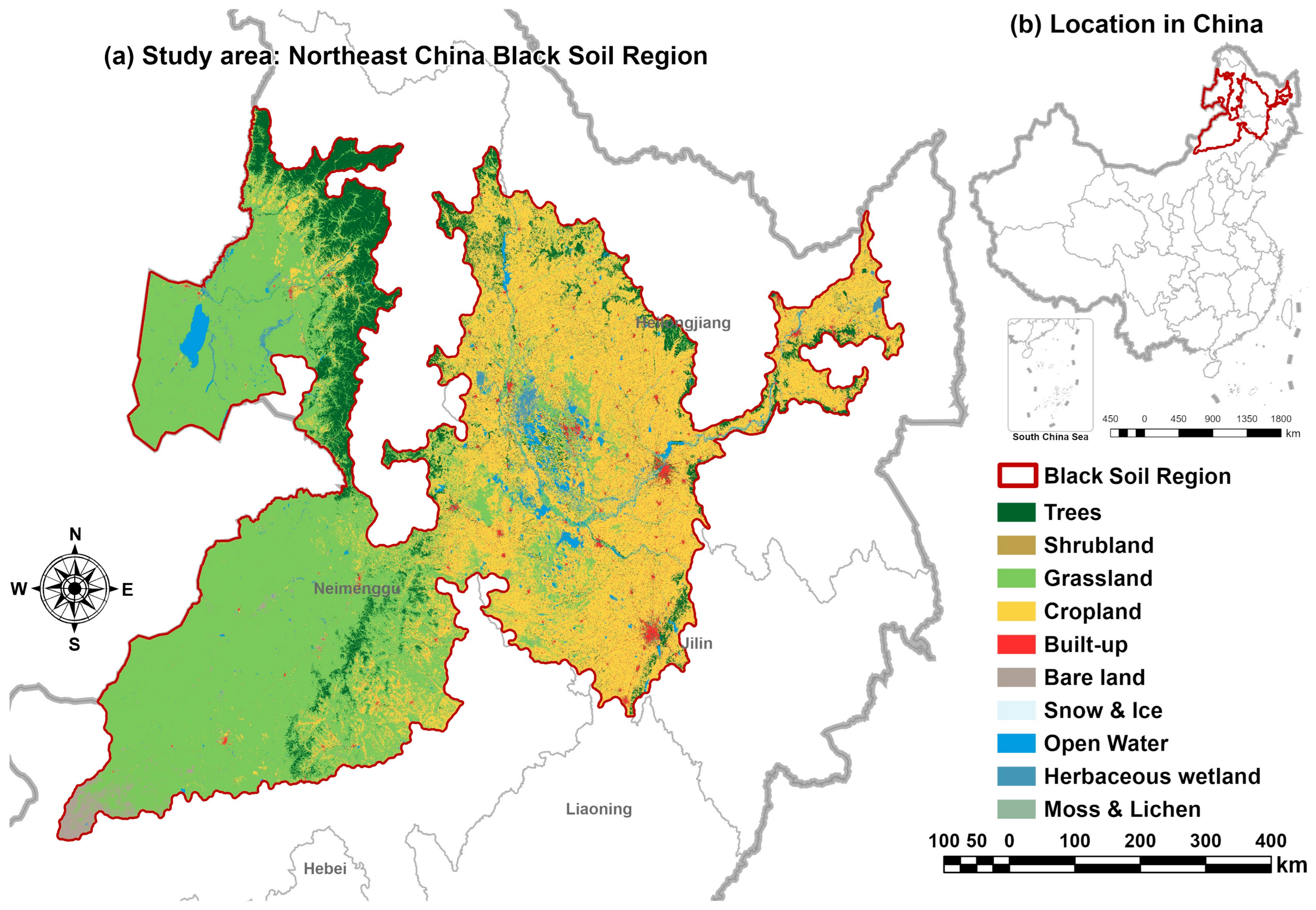
Figure 1. Study area location, boundary of the black soil region in Northeast China, and major land-cover classes. (a) Major land-cover classes within the black soil region boundary; (b) location of the study area within China.
Land 15 01292 g001
Figure 2. RUSLE-GEE technical workflow for multi-temporal diagnosis of cropland water erosion. The workflow summarizes the study-area boundary and cropland masks, remote-sensing and geospatial data inputs, R, K, LS, C, and P-factor parameterization in GEE, six diagnostic time slices, P-factor scenario tests, rainfall-source and cropland-mask sensitivity analyses, and interpretation of results and uncertainty boundaries.
Land 15 01292 g002
Figure 3. Spatial distribution of the five RUSLE factors in 2024 and their pixel-level coupling with soil loss. (a) Spatial distribution of the R factor in 2024, representing spatial variation in rainfall erosivity; (b) spatial distribution of the K factor, representing variation in soil erodibility; (c) spatial distribution of the LS factor, shown on a logarithmic scale to highlight the low-value topographic background and localized high values; (d) spatial distribution of the C factor, reflecting vegetation cover and cover-management conditions; (e) spatial distribution of the P factor under the slope-graded P-factor scenario; and (f) pixel-level Spearman rank correlation ordering between the five factors and 2024 SL, summarizing the relative coupling strength between model inputs and the spatial pattern of SL.
Land 15 01292 g003
Figure 4. Integrated diagnosis of R, C, SL, and erosion-grade structure across six time slices. (a) R-C bivariate bubble trajectory plot, with R (MJ mm ha−1 h−1 yr−1) on the x-axis, dimensionless C on the y-axis, bubble size representing SLmean (t ha−1 yr−1), and gray lines showing the discrete temporal path; (b) ridge plot of the pixel-level SL distribution, comparing years on a logarithmic scale and marking the T = 2 t ha−1 yr−1 threshold; (c) faceted area-share plots for erosion grades, showing the structure of very slight, slight, moderate, and intense-or-higher erosion across six years; and (d) beanplot and boxplot combination for the pixel-level SL distribution, comparing distributional shape, dispersion, and mean position among years.
Land 15 01292 g004
Figure 5. Spatial distribution of annual cropland soil loss (t ha−1 yr−1) in the black soil region of Northeast China, 2001–2024. Panels (af) show the classified spatial distribution of annual cropland soil loss in 2001, 2005, 2010, 2015, 2020, and 2024, respectively, with colors from green to red indicating increasing SL. The bottom color bar gives the SL class thresholds; the inset line chart summarizes changes in SLmean across the six time slices; and the bar and stacked-bar insets summarize the over-T percentage and erosion-grade area structure. The figure is used primarily to show the location of high-SL zones and their variation among the six discrete years.
Land 15 01292 g005
Figure 6. Risk matrix stratified by slope band, area–intensity relationship, and 2024 slope band diagnosis. (a) Risk matrix combining six time slices and six slope bands, with cell color and values representing SLmean (t ha−1 yr−1) and circle size representing the over-T percentage (%); (b) distributional summary of SL within each 2024 slope band, where points indicate means and horizontal lines indicate available p50–p95 percentile ranges, with T = 2 t ha−1 yr−1 as a reference; (c) log–log relationship between 2024 slope band area share and SLmean, with point size representing the over-T percentage (%), highlighting that high-slope bands occupy little area but have high per-area intensity; and (d) comparison between slope band area share and area-weighted SL contribution, showing that both area base and per-area intensity jointly determine the overall contribution of each slope band. In panels (bd), colors consistently distinguish the six slope bands from <2% to ≥20%.
Land 15 01292 g006
Figure 7. Evidence summary for P-factor scenarios, slope units, cropland masks, and rainfall-source sensitivity. (a) Summary of relative effect magnitude (%) by evidence type and direction for P-factor scenarios, P-factor slope-unit implementation, rainfall-source substitution, and cropland-mask replacement on SLmean; (b) difference in SLmean (t ha−1 yr−1) between the p = 1.0 no-practice scenario and the slope-graded P-factor scenario across six time slices, with the shaded area representing the structural envelope introduced by P-factor parameterization, the red and gray lines denote the no-practice and slope-graded P-factor scenarios, respectively; (c) relative differences in cropland area (%), SLmean (%), and the over-T percentage (percentage points) under the GLC FCS30D dynamic cropland mask relative to the ESA WorldCover 2021 static mask; and (d) relationship between Rmean (MJ mm ha−1 h−1 yr−1) and SLmean (t ha−1 yr−1) under CHIRPS, GPM IMERG, and ERA5-Land rainfall forcing in 2024, with the current main diagnostic result marked as a reference.
Land 15 01292 g007
Figure 8. Endpoint diagnosis of SL difference, over-T state transition, and pixel-level endpoint relationship between 2001 and 2024. (a) Spatial endpoint difference map showing (SL2024 − SL2001; t ha−1 yr−1), where blue indicates lower SL in 2024 than in 2001 and red indicates higher SL in 2024; (b) endpoint state transition under the T = 2 t ha−1 yr−1 threshold, distinguishing persistently below-threshold, newly over-T, transitioned from over-T to below-T, and persistently over-T states; and (c) pixel-level endpoint relationship between log10-transformed SL in 2001 and 2024 with marginal distributions, with SL expressed in t ha−1 yr−1 before transformation, used to assess the overall relationship, density clustering, and deviations from the 1:1 line, the blue top and red right histograms represent the marginal distributions of log10-transformed SL in 2001 and 2024, respectively, while the blue shading and contours indicate the joint pixel density.
Land 15 01292 g008
Figure 9. Ternary spatial diagnosis of R-C-SL combinations and threshold-response patterns in 2024. (a) Spatial diagnostic zoning map, in which R (MJ mm ha−1 h−1 yr−1) and dimensionless C are split into high and low groups using effective-pixel medians and combined with the SL threshold T = 2 t ha−1 yr−1 to form eight R-C-SL states; (b) ternary phase diagram based on robustly scaled R, C, and SL intensities, with blue shading and contours indicating pixel density and centroid colors corresponding to the eight states in (a); and (c) R-C quadrant ring diagram, in which the inner ring represents the four R-C quadrants and the outer ring distinguishes ≤T and >T states using the colors in (a).
Land 15 01292 g009
Table 1. Temporal treatment of RUSLE factors across the six diagnostic years.
FactorUnitData SourceTemporal TreatmentExplanation
RMJ mm ha−1 h−1 yr−1CHIRPS Daily precipitationDynamicCalculated for each diagnostic year.
Kt h MJ−1 mm−1SoilGrids 250 mStaticBaseline soil texture and SOC; the same K map was used for all time slices.
LSDimensionlessSRTM DEMStaticTopographic factor derived from the DEM.
CDimensionless (0–1)Landsat NDVIDynamicCalculated for each diagnostic year using monthly vegetation cover and R weighting.
PDimensionless (0–1)Slope-grade ruleStatic/scenario-basedSupport-practice scenario based on slope classes; not an observed year-by-year conservation-practice map.
Disclaimer/Publisher’s Note: The statements, opinions and data contained in all publications are solely those of the individual author(s) and contributor(s) and not of MDPI and/or the editor(s). MDPI and/or the editor(s) disclaim responsibility for any injury to people or property resulting from any ideas, methods, instructions or products referred to in the content.