Multi-Source Weighting Integration for Evaluating the Eco-Geological Environmental Carrying Capacity in Kunming, China

Abstract

Eco-geological environmental carrying capacity (EGECC) refers to the ability of a regional eco-geological environmental system to support human activities and socioeconomic development while maintaining ecological functions and geological stability. Its assessment is important for preventing geological hazards, regional development, and the green transition. However, existing studies often face challenges, such as subjectivity in assigning weights and limited capacity to capture nonlinear interactions among multiple factors. To address these limitations, this study focuses on Kunming City. It applies the analytic hierarchy process and coefficient of variation methods to derive subjective and objective weights, respectively. At the same time, random forest is used to identify nonlinear indicator contributions embedded in the evaluation results. These weights are then integrated through an improved linear efficacy coefficient framework to construct a comprehensive weighting scheme. The results indicate that Kunming’s EGECC shows a spatially heterogeneous pattern, with higher values distributed mainly in the southeastern and southwestern areas, especially in Shilin County. In contrast, lower values are concentrated in the northern mountainous areas and highly urbanized central districts, such as Dongchuan and Wuhua Districts. Moreover, spatial pattern detection of the EGECC is sensitive to the choice of composite weighting method, while interactions among geological factors—such as disaster point density and slope—play a major role in shaping the carrying capacity. Overall, the proposed composite weighting approach provides a relatively balanced integration of expert-knowledge-based, data-dispersion-based, and nonlinear data-driven information, and its reliability is further examined through geological hazard-point validation and weight-perturbation sensitivity analysis.

1. Introduction

With advancements in ecological geology since the 1930s and in environmental geology since the 1970s, researchers have gradually improved their understanding of the eco-geological environment. It is now regarded as an integrated system encompassing geological, ecological, and socioeconomic dimensions [1]. The concept of eco-geological environmental carrying capacity (EGECC) has developed from earlier research on geological and ecological carrying capacities [2]. It refers to the capacity of an eco-geological system to accommodate external environmental changes and human disturbances while maintaining fundamental structural stability and supporting socioeconomic development within a defined spatial and temporal scope [3]. In this study, the term “eco-geological environmental carrying capacity” (EGECC) follows the terminology used in previous studies. It refers to the integrated carrying capacity of an environmental system jointly shaped by geological conditions, ecological processes, and socioeconomic activities. Therefore, the word “environmental” is retained to emphasize the broader environmental context formed by the interaction of geological, ecological, and human activity subsystems. While research on ecological carrying capacity is relatively well established, studies of geological carrying capacity are less developed. Assessing the EGECC by integrating geological, ecological, and socioeconomic subsystems involves handling multi-source data and methodological complexity. Early international efforts primarily linked carrying capacity to hydrology [4], soil science [5], ecology [6], tourism [7], and cultural studies [8]. Since the 2010s, increasing attention has been given to regional-scale assessments, particularly those concerning ecological, geological, and urban environmental capacities [9]. Owing to its inherently interdisciplinary nature, EGECC research still faces challenges in constructing robust evaluation index systems, integrating diverse indicators, and selecting appropriate assessment models [10]. As scholarship has advanced, accurately evaluating the EGECC and providing scientific references for regional development planning have become important issues in both academic and policy-oriented contexts. In response, various weighting techniques and modeling approaches have been proposed, thereby gradually expanding the theoretical and methodological foundation.

Weighting methods used in carrying capacity assessment generally include subjective, objective, and hybrid approaches. Commonly used methods include the analytic hierarchy process (AHP, an expert-judgment-based weighting method) [11,12], the entropy weight method (an objective method based on information dispersion) [13,14], the CRITIC method (an objective method considering contrast intensity and conflicts among indicators) [15], TOPSIS (a multi-criteria decision-making method based on distance from ideal solutions) [16], principal component analysis (PCA, a dimensionality-reduction method) [17], and the coefficient of variation (CV) method (an objective weighting method based on relative variability) [18]. Assessment frameworks often rely on composite index models [19], fuzzy comprehensive evaluation [20], PSR models [21], gray system theory [22], set pair analysis [23], and system dynamics [24].

The AHP, developed by Saaty in the 1970s, decomposes complex decisions into hierarchical structures that combine qualitative and quantitative analyses [25], although it is often noted for its subjectivity [26,27]. In this context, subjectivity or subjective bias refers to the influence of expert preferences, prior assumptions, or judgment inconsistencies on the assignment of indicator weights. The entropy weight method, derived from Shannon’s information theory [28], is valued for its theoretical basis but may be sensitive to data distribution and computationally less efficient [29]. The CRITIC method [30] uses contrast intensity and inter-attribute correlation to assign objective weights. Techniques such as TOPSIS [31] and PCA enable multi-criteria evaluation and dimensionality reduction but may be constrained by sensitivity and interpretability issues [32,33]. Here, sensitivity means that small changes in input data, normalization methods, or classification thresholds may alter the final ranking or classification results. In contrast, interpretability refers to the difficulty of directly linking transformed or aggregated results to specific eco-geological processes. The CV method [34] highlights indicator variability but may be less effective when applied to systems with many indicators or complex interrelationships [35]. Integrating subjective and objective methods, often combined with GIS for spatial analysis, has become a common practice in EGECC evaluation [36,37,38,39].

However, traditional models often overlook complex coupling and nonlinear interactions between ecological and geological indicators, limiting their ability to reflect ecosystem processes in detail [40]. In recent years, machine learning approaches, particularly random forest (RF), have been adopted because of their ability to capture nonlinear patterns and highlight influential indicators within multidimensional datasets [41]. Although composite weighting schemes have been introduced to mitigate the biases inherent in single-method weighting, studies that integrate subjective, objective, and data-driven approaches into a unified framework remain relatively scarce. The modified linear efficacy coefficient method offers one possible pathway for integrating multiple sources of weight information.

Moreover, identifying the spatial drivers of the EGECC through statistical models has become an important research focus. Commonly used approaches include the obstacle degree model [42], geographically weighted regression [43], spatiotemporally weighted regression [44], and the geographic detector model [45]. 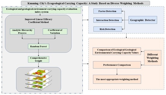GeoDetector, developed by Wang Jingfeng and Xu Chengdong, is widely applied for quantifying spatial heterogeneity and exploring driving mechanisms in complex systems [46] and is being increasingly applied in carrying capacity analysis [43,47,48]. Nevertheless, studies that combine multi-source weighting integration with spatial heterogeneity analysis remain limited, especially in plateau cities with complex geological backgrounds, rapid urbanization, and fragile ecological conditions. This study focuses on Kunming City and develops an evaluation index system with 14 indicators spanning geological, ecological, and socioeconomic dimensions to assess the EGECC. The AHP and CV methods are used to derive subjective and objective weights, respectively. In contrast, RF is introduced to identify nonlinear indicator contributions embedded in the AHP- and CV-derived evaluation results. A comprehensive weighting method based on an improved linear efficacy coefficient framework is then used to integrate the three weighting results. The composite index model is applied to evaluate the EGECC under different weighting schemes, and the spatial patterns are compared across methods. In combination with the GeoDetector model, factor, interaction, and risk detection are used to examine the driving forces and regional variations influencing the EGECC. This study aims to provide a balanced multi-source weighting framework and practical reference for eco-geological conservation and sustainable regional development.

2. Study Area

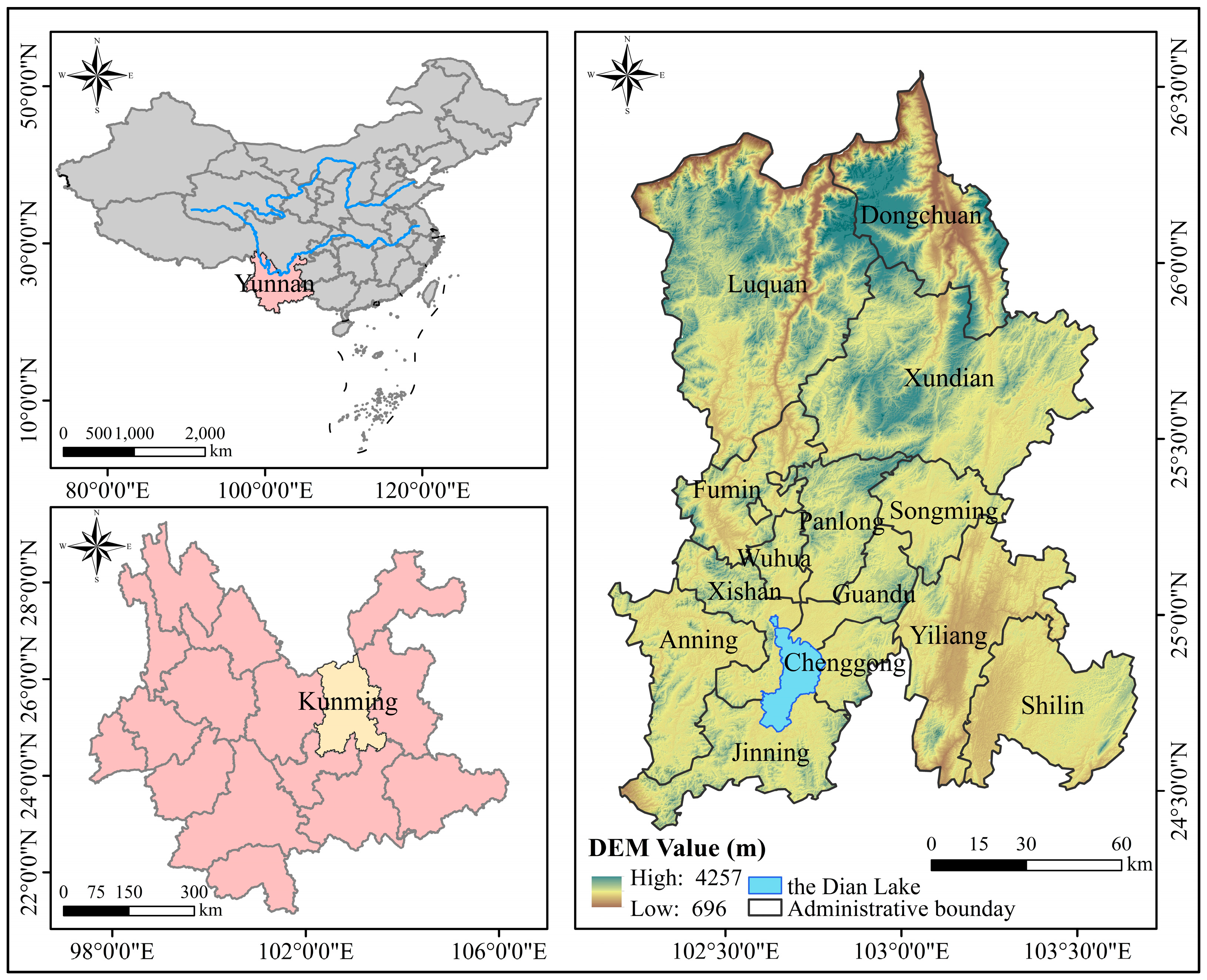
Kunming City is located in the central Yungui Plateau of southwestern China, between 102°10′–103°40′ E and 24°23′–26°22′ N. It includes seven urban districts (Wuhua, Panlong, Guandu, Xishan, Dongchuan, Chenggong, and Jinning), three counties (Fumin, Yiliang, and Songming), three autonomous counties (Shilin Yi Autonomous County, Luquan Yi and Miao Autonomous County, and Xundian Hui and Yi Autonomous County), and one county-level city (Anning), covering an area of about 21,012.54 km². Owing to its geographic location, Kunming functions as a regional center for international economic and trade cooperation and as a gateway to Southeast Asia, South Asia, and other regions. Situated on the Yungui Plateau, Kunming’s topography is characterized by higher elevations in the north that gradually decrease in a step-like pattern toward the south, with central uplifted terrain and relatively lower areas to the east and west. Most areas range in altitude between 1500 and 2800 m (see Figure 1 for geographic context). The main urban area lies within the Kunming Basin, a geologically complex basin at the southern end of China’s north–south tectonic belt, marked by widespread lacustrine landforms and relatively weak substrata. The city has diverse stratigraphic sequences, including deposits from the Quaternary, Tertiary, Jurassic, Triassic, Permian, Carboniferous, Devonian, Silurian, Ordovician, Cambrian, Sinian, and Kunyang Groups.

Kunming has a highland subtropical monsoon climate, with mild summers and winters that are not severely cold. The annual mean temperature is about 15.7 °C, with maximum temperatures generally below 30 °C and minimum temperatures typically above 0 °C. The city experiences distinct wet and dry seasons and frequent winds, which has led to its designation as the “spring city.” In recent decades, economic growth and increased human activities have introduced pressures on both geological and ecological systems. Therefore, evaluating the ecological–geological environmental carrying capacity of Kunming is relevant to understanding land-use challenges and supporting balanced human–environment interactions.

3. Materials and Methods

3.1. Data Sources

The dataset used in this study comprises fundamental geographic, geological, ecological, meteorological, hydrological, and socioeconomic data. These data were obtained through field surveys, institutional data collection, and multichannel online sources. The digital elevation model (DEM) was obtained from the European Space Agency’s Copernicus DEM dataset at a 30 m spatial resolution and used to derive elevation and slope. Geological hazard-point data for Kunming City were provided by the Kunming Natural Resources and Planning Bureau and represent the latest available hazard inventory around the assessment period. Lithological and structural data, including engineering geological rock groups and faults, were derived from 1:200,000 regional geological maps and were treated as static geological background data. Meteorological data, including average annual precipitation and average annual temperature, were obtained from the Geographic Remote Sensing Ecology Network and were calculated using annual or multiyear average climate data corresponding to the study period. Road network and hydrographic data were extracted from the 1:250,000 National Basic Geographic Database, available through the National Geographic Information Resource Directory Service System. They were used to calculate road density and distance to water systems. The land resource classification dataset was derived from the Esri 10 m land cover dataset and used in conjunction with DEM-derived slope to characterize farmland conditions. Vegetation coverage and the normalized difference built-up index (NDBI) were extracted from Landsat 8–9 OLI/TIRS C2 L1 satellite imagery acquired around 2022 and downloaded from the U.S. Geological Survey (USGS) platform, with ENVI 5.3 used for band extraction and ArcGIS 10.7 used for subsequent spatial processing. Population and GDP data were collected from the 2022 Kunming National Economic and Social Development Statistical Bulletin and used to calculate population and GDP densities. Unless otherwise specified, all online datasets and web-based resources used in this study were accessed between 1 May 2024 and 31 May 2024.

To improve temporal consistency, the EGECC evaluation was conducted mainly using the latest available datasets from about 2022. Socioeconomic indicators, including population density and GDP density, were derived from 2022 statistical data, whereas vegetation coverage and the NDBI were extracted from Landsat imagery acquired around the same assessment period. Relatively stable background indicators, including DEM, slope, engineering geological rock groups, distance to faults, distance to water systems, road density, and geological hazard points, were treated as static or quasi-static variables because they changed slowly over the assessment period or represent the latest available baseline conditions. Although the datasets differ in temporal frequency and spatial resolution, all spatial data were projected into a unified coordinate system, resampled or converted as needed, and clipped to the administrative boundary of Kunming City before subsequent analysis.

3.2. Research Methods

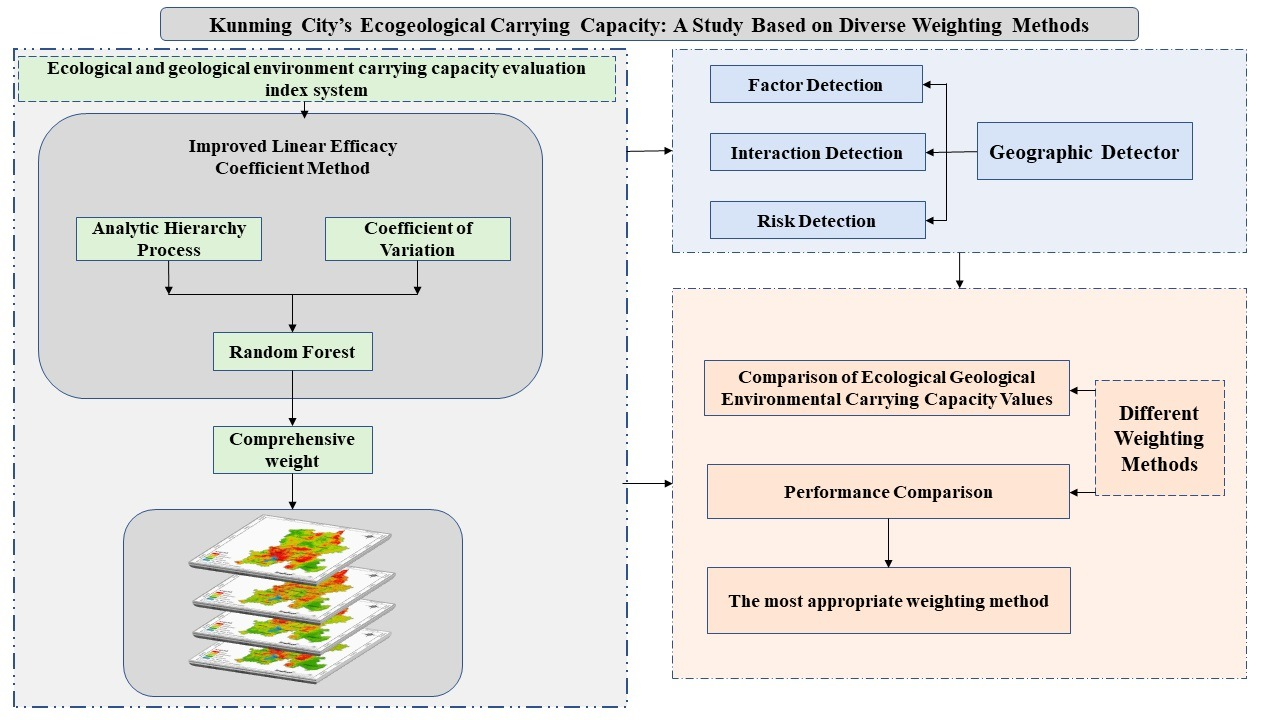
The methodological framework was organized into five analytical steps. First, the AHP and CV were used to derive subjective and objective weights, respectively, whereas RF was used to identify nonlinear indicator contributions embedded in the AHP- and CV-derived evaluation results. Second, the improved linear efficacy coefficient framework was used to integrate the three weighting results into a comprehensive set of weights. Third, the composite index model was applied to map the spatial distribution of the EGECC. Fourth, spatial autocorrelation analysis was used to identify whether high or low EGECC values were spatially clustered at the county/district level. Fifth, GeoDetector was used to explain spatial heterogeneity by identifying dominant factors, factor interactions, and interval-related differences. Finally, validation and sensitivity analyses were conducted to assess the reliability and robustness of the evaluation results. The analytic hierarchy process (AHP) and coefficient of variation (CV) methods represent common subjective and objective weighting approaches, respectively, and will not be further elaborated here; detailed computational procedures can be found in the relevant literature [49,50].

3.2.1. Random Forest

Random forest (RF) is a robust ensemble learning algorithm [51]. Its underlying principle is to employ bootstrap sampling to randomly extract subsets of the training data for constructing individual trees. During the node splitting process, a randomly selected subset of features is evaluated, and the final prediction is determined as the average of all individual tree outputs.

$$IG(T,A)=H(T)-\sum _{v\in Values(A)}{\displaystyle \frac{\left|T_v\right|}{\left|T\right|}}H(T_v)$$

(1)

$$Gini(T)=1-{\sum }_{i=1}^C{p}_i^2$$

(2)

$$Importance(A)={\displaystyle \frac{1}{N}}{\sum }_{i=1}^N({{OOB}_{error}}^{(i)}(A)-{{OOB}_{error}}^{(i)})$$

(3)

In the formula, $H(T)$ denotes the entropy of the dataset $T$. $A$ represents a feature, and $Values(A)$ comprises all possible values of this feature. $T_v$ refers to the subset of $T$ for which feature $A$ takes the value $v$. $C$indicates the number of classes, whereas $p_i$ is the proportion of class $i$ within $T$. $N$represents the number of trees. ${{OOB}_{error}}^{(i)}$ represents the prediction error of the i-th tree on its corresponding out-of-bag (OOB) samples, whereas ${{OOB}_{error}}^{(i)}(A)$ denotes the prediction error recalculated after permuting the values of feature A.

3.2.2. Improved Linear Efficacy Coefficient Method

In the classical linear efficacy coefficient method, the combined weight $W_i$ is computed as the weighted average of the subjective weight $W_{i1}$ and the objective weight $W_{i2}$. To further increase the method’s flexibility and accuracy, this study introduces a third weight $W_{i3}$ so that the combined weight can comprehensively incorporate three different sources of weight information. The improved combined weight calculation formula is as follows:

$$\alpha +\beta +\gamma =1$$

(4)

$$W_i={\alpha W}_{i1}+{\beta W}_{i2}+\gamma W_{i3}$$

(5)

$$L(\alpha ,\beta ,\gamma ,\lambda )={\displaystyle \frac{1}{2}}{\displaystyle \sum _{i=1}^n}{((W_{i1}-W_i)}^2+{(W_{i2}-W_i)}^2+{(W_{i3}-W_i)}^2)+\mathsf{\lambda }(\alpha +\beta +\gamma -1)$$

(6)

Here, $W_i$ denotes the combined weight of the $i$th indicator, whereas $W_{i1}$, $W_{i2}$, and $W_{i3}$ represent the weights of the ith indicator obtained from the three methods. The variable $n$ indicates the total number of evaluation indicators, and $\alpha$, $\beta$, and $\gamma$ are the allocation coefficients used in computing the combined weight.

In this study, the improved linear efficacy coefficient method was used as a general framework for integrating three sources of weights. Because AHP, CV, and RF represent expert-knowledge-based, data-dispersion-based, and nonlinear data-driven perspectives, respectively, and because no independent benchmark was available for calibrating adaptive coefficients, equal allocation coefficients were adopted, namely, α = β = γ = 1/3. This setting avoids assigning additional subjective preferences to any single weighting method and ensures that the final comprehensive weight reflects a balanced integration of the three weighting sources. Therefore, the comprehensive weight can be expressed as follows:

$$W_i={(W}_{i1}+W_{i2}+W_{i3})/3$$

(7)

where ${\mathrm{W}}_{i1}$, ${\mathrm{W}}_{i2}$, and ${\mathrm{W}}_{i3}$ represent the AHP, CV, and RF weights of the ith indicator, respectively.

3.2.3. Spatial Autocorrelation

Spatial autocorrelation is a fundamental tool for examining the degree to which similar values of a variable are clustered in space [52]. In this study, both global and local measures of spatial autocorrelation, namely, Global Moran’s I and Local Moran’s I, were calculated to assess the spatial patterns of eco-geological carrying capacity across the study area.

(1) The global Moran’s I statistic is used to quantify the overall spatial autocorrelation of a variable across the entire study region [53]. It is defined as

$$I={\displaystyle \frac{n}{W}}{\displaystyle \frac{{\sum }_{i=1}^n{\sum }_{j=1}^n{w}_{ij}(x_i-\overline{x})(x_j-\overline{x})}{{\sum }_{i=1}^n{(x_i-\overline{x})}^2}}$$

(8)

where $n$ is the number of spatial units, $x_i$ is the observed value at location $i$, $\overline{x}$ is the mean value of the variable, $w_{ij}$ is the spatial weight between locations i and j, and $W={\sum }_{i=1}^n{\sum }_{j=1}^n{w}_{ij}$ is the sum of all spatial weights. A positive value of I indicates that similar values (either high or low) tend to cluster in space, whereas a negative value suggests a dispersed pattern. A value near zero indicates spatial randomness. The significance of I is typically assessed via a permutation test to obtain a p value.

(2) While the global measure provides an overall indication of spatial autocorrelation, it does not reveal local patterns of clustering. Therefore, local Moran’s I is computed for each spatial unit i as [54]

$$m_2={\displaystyle \frac{1}{n}}{\displaystyle \sum _{i=1}^n}{(x_i-\overline{x})}^2$$

(9)

$$I_i={\displaystyle \frac{(x_i-\overline{x})}{m_2}}{\sum }_{j=1}^n{w}_{ij}(x_j-\overline{x})$$

(10)

where $I_i$ is local Moran’s I for unit i and where $m_2$ is the variance of the variable.

Local Moran’s I identifies the presence of spatial clusters and outliers. Typically, the results are categorized into four types on the basis of the sign and significance of $I_i$ and the standardized values $z_i={\displaystyle \frac{x_i-\overline{x}}{\mathsf{\sigma }}}$:

• High–High (HH): A unit with a high value is surrounded by other high values, indicating a hotspot.
• Low–Low (LL): A unit with a low value is adjacent to other low values, indicating a cold spot.
• High–Low (HL): A unit with a high value is surrounded by low values, indicating a potential spatial outlier.
• Low–High (LH): A unit with a low value is adjacent to high values, also indicating an outlier.

The significance of each $I_i$ is assessed via permutation tests, and only values with p values below a chosen threshold (e.g., 0.05) are considered statistically significant.

3.2.4. Geographic Detector

Geographic detector is a statistical analysis method used to detect the spatial distribution characteristics of geographic phenomena and their influencing factors. Analyzing the spatial consistency of variables can identify potential driving forces and is suitable for studying complex natural and social phenomena. Geographic detector includes four main modules: factor detection, interaction detection, risk detection, and ecological detection. In this paper, only the first three modules are used. Ecological detection was not included because this study focused on factor explanatory power, factor interactions, and interval-related differences rather than on pairwise significance comparisons between the effects of different factors. Therefore, factor, interaction, and risk detection were selected to align with the research objectives.

(1) Factor detector: This module is used to assess the spatial consistency between the dependent and independent variables. A commonly used q value calculation formula is as follows:

$$q=1-{\displaystyle \frac{{\sum }_{h=1}^L{N}_h{\sigma }_h^2}{N{\sigma }^2}}$$

(11)

The q value is the factor detector value, representing the degree of spatial heterogeneity in the dependent variable explained by the independent variable. Its range is [0, 1], where a higher q value indicates stronger explanatory power of the independent variable. L represents the number of categories into which the dependent variable is divided. $N_h$ is the number of samples in the hth category, and ${\sigma }_h^2$ is the variance of the dependent variable within the hth category. $N$ is the total number of samples, and ${\sigma }^2$ is the overall variance of the dependent variable.

(2) The interaction detector identifies the influence of interactions between two factors on the dependent variable. It examines whether the interaction between two independent variables enhances or weakens their effect on the dependent variable. The interaction detector calculates the q value for the combination of two variables and compares it with the q value of a single variable. Interaction effects are classified as enhancement, weakening, or nonlinear enhancement.

(3) The risk detector analyzes whether the mean differences in the dependent variable among different groups are statistically significant. T-tests or analysis of variance (ANOVA) are typically used for significance testing, allowing an examination of differences in the effect of a given factor on the dependent variable across groups.

3.3. Data Processing

The analysis was conducted at two spatial levels. First, the raster-based indicators were resampled to a consistent spatial resolution and used to generate continuous EGECC maps. The area proportions of different EGECC classes were calculated at the raster level. Second, county/district-level statistics were derived using zonal statistics to compare administrative units and to conduct county-level spatial autocorrelation analysis. Therefore, the raster scale was used for spatial mapping and classification, whereas the county/district scale was used for regional comparison and spatial autocorrelation analysis.

3.3.1. Selection of Evaluation Indicators

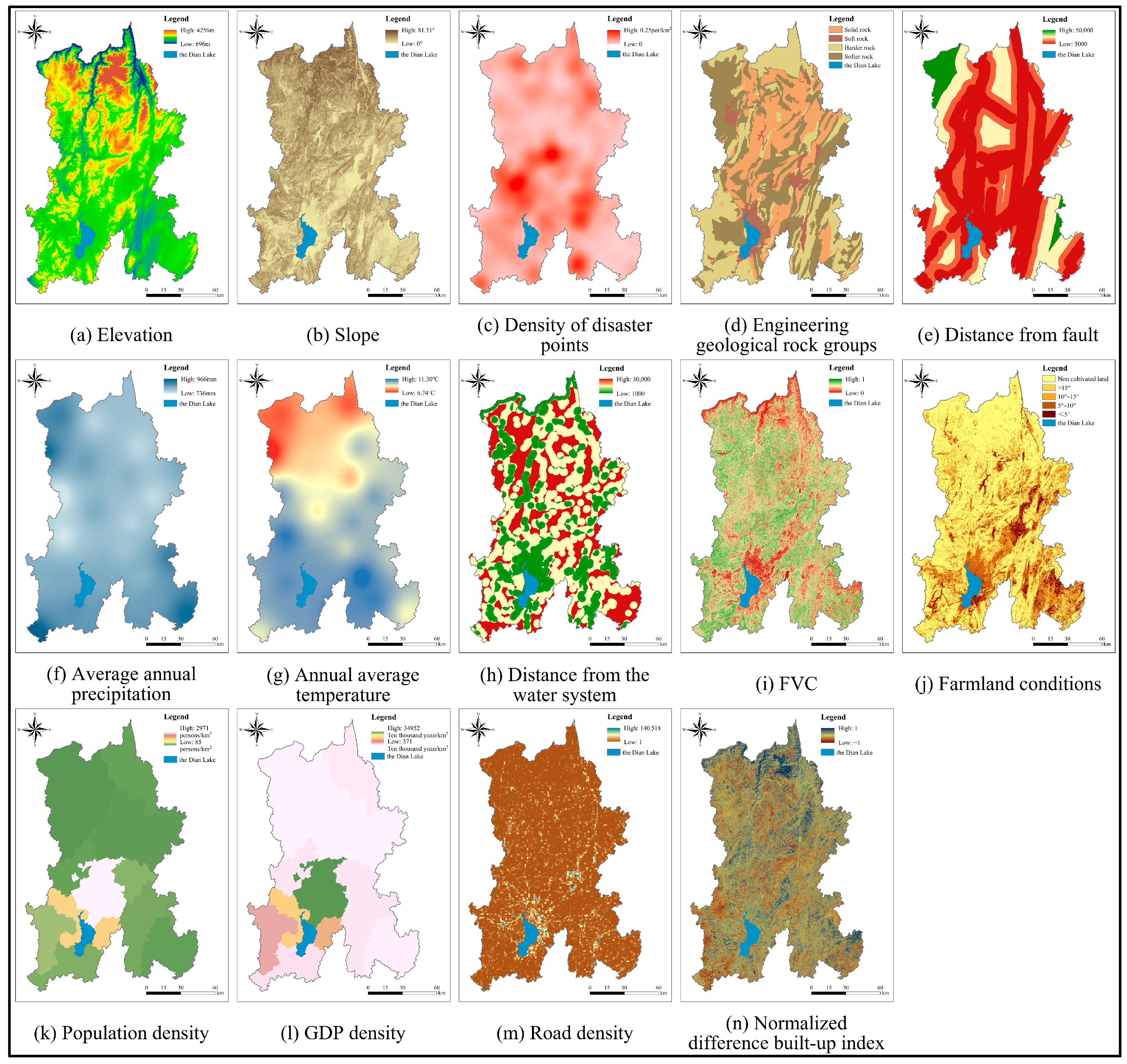
The selection of evaluation indicators is a critical step in ensuring the reliability of EGECC assessments. The primary research objective is to evaluate the balance between human activities and the environment, and the choice of indicators directly influences how well the results reflect local conditions. Drawing on evaluation frameworks established in previous studies on eco-geological environmental carrying capacity and considering the specific environmental characteristics of Kunming, 14 indicators were selected. These indicators are grouped into three dimensions: the geological, ecological, and socioeconomic environments. The selected indicators include elevation, slope, density of hazard points, geological rock formations, distance to fault lines, average annual precipitation, average annual temperature, distance to water systems, vegetation coverage, arable land conditions, population density, GDP per capita, distance to roads, and the building index. Together, these factors form the evaluation indicator system for Kunming City’s EGECC [3,11,16,55,56,57,58,59]. To ensure the robustness and independence of the selected indicators, a multicollinearity test was conducted before model construction. A Variance Inflation Factor (VIF) analysis was applied to assess the degree of collinearity among the variables. The results showed that all indicators had VIF values below the commonly accepted threshold (VIF < 10), indicating no significant multicollinearity among the variables. Therefore, all selected indicators were retained for subsequent analysis. The spatial distributions of these indicators are presented in Figure 2.

3.3.2. Indicator Classification

As an important factor influencing regional socioeconomic development, the magnitude of the EGECC is determined by multiple indicators. Elevation and slope are generally negatively correlated with geological environmental carrying capacity. The geological environment dimensions include the distance to faults, geological engineering rock formations, and hazard-point density. Geological hazard points are used as indicators of geological environment quality and carrying capacity, as their frequent occurrence may suggest unfavorable geological conditions and lower carrying capacity. The ecological environment is represented by precipitation, temperature, vegetation coverage, distance to water systems, and arable land conditions. Higher precipitation, relatively favorable temperatures, greater vegetation coverage, lower slopes under arable land use, and closer proximity to water systems are generally associated with better ecological environmental carrying capacity. The socioeconomic environment dimension includes population density, GDP density, road density, and the building index. In this context, lower population pressure, stronger socioeconomic support capacity, weaker construction disturbance, and reduced excessive road-related disturbance are considered more favorable for socioeconomic environmental carrying capacity. Because these indicators have different units and ranges, standardization is required to ensure comparability. The indicators were classified into two categories based on their relationship with the EGECC: positive and negative indicators. Positive indicators are those for which an increase in the indicator value is generally associated with an increase in the carrying capacity. Negative indicators are those for which an increase in the indicator value is generally associated with a decrease in carrying capacity; in other words, lower values of negative indicators correspond to more favorable carrying capacity conditions. The characteristics of the evaluation indicators are summarized in

Table 1. Nature of the evaluation indicators.

Criterion Layer	Index Level	Index Type
Geological environment	Elevation D1 (m)	Lower elevation generally indicates fewer topographic constraints
	Slope D2 (°)	Lower slope generally indicates better terrain stability and suitability
	Density of disaster points D3 (per/km2)	Lower hazard-point density indicates lower geological hazard pressure
	Engineering geological rock groups D4	Harder rock groups indicate better engineering geological stability
	Distance from fault D5 (m)	Greater distance from faults indicates lower tectonic disturbance
Ecological environment	Average annual precipitation D6 (mm)	More favorable precipitation conditions indicate better ecological support capacity
	Annual average temperature D7 (°C)	More favorable thermal conditions indicate better ecological suitability
	Distance from the water system D8 (m)	Shorter distance to water systems indicates better water-resource accessibility
	FVC D9	Higher vegetation coverage indicates better ecological condition
	Farmland conditions D10 (°)	Lower slope under cultivated land conditions indicates better farmland suitability
Social economy	Population density D11 (person/km2)	Lower population density indicates lower human pressure
	GDP density D12 (ten thousand yuan/km2)	Higher GDP density indicates stronger socioeconomic support capacity
	Road density D13	Excessive road density indicates stronger human disturbance
	NDBI D14	Lower NDBI indicates weaker construction

.

The direction and interpretation of each indicator were determined based on previous EGECC studies, the environmental characteristics of Kunming, and the practical meaning of each variable in relation to the carrying capacity. For indicators such as slope, hazard-point density, distance to faults, population density, and the NDBI, the assumed relationships with the EGECC are relatively clear. However, some indicators, such as temperature, precipitation, GDP density, and road density, may have nonlinear or threshold effects. In this study, these indicators were classified using interval-based grading rather than continuous monotonic functions, which partially reduced the oversimplification caused by direct linear standardization.

When evaluation indicators are quantitatively processed, specific numerical values are assigned to each indicator according to defined standards. The indicator scaling method is applied within the evaluation system, taking into account each indicator’s contribution, effect, and potential influence on the stability of the EGECC. The classification thresholds were determined by integrating the natural breaks of the raster values within Kunming City, which are commonly used grading standards in previous EGECC studies, and local environmental characteristics such as plateau topography, geological hazard background, and urban development intensity. Following the classification standards of the natural break method, values ranging from 1 to 4 are used: “Excellent” is assigned a value of 4, “Good” a value of 3, “Moderate” a value of 2, and “Poor” a value of 1. Comparisons are conducted vertically and horizontally across indicator levels to guide assignment, aiming to enhance consistency and comparability. The assignment results are presented in

Table 2. Index assignment grading table.

Index Level	Level 1	Level 2	Level 3	Level 4
D1	>2800	2200–2800	1800–2200	<1800
D2	>30	20–30	10–20	0–10
D3	>0.14	0.08–0.14	0.04–0.08	0–0.04
D4	Soft rock	Softer rock	Harder rock	Solid rock
D5	<500	500–1000	1000–1500	>1500
D6	<800	800–840	840–880	>880
D7	<8	8–9	9–10	>10
D8	>16,000	3000–16,000	1500–3000	<1500
D9	0–0.25	0.25–0.50	0.50–0.75	0.75–1
D10	>15	10–15	5–10	<5
D11	>1000	300–1000	200–300	<200
D12	<1500	1500–5200	5200–14,000	>14,000
D13	>6	4–6	2–4	0–2
D14	>0.025	−0.05–0.025	−0.1–−0.05	<−0.1

.

3.3.3. Determination of Indicator Weights

The combined weighting method, which integrates the AHP and CV approaches, is typically applied to obtain subjective and objective weights. In this study, the EGECC grading results derived separately from the AHP weights and CV weights were used as the target variables, and the indicators were treated as predictor variables. The RF method was then employed for training. Following the random sampling principle in RF, 70% of the evaluation units were randomly selected (without replacement) from each of the two result sets and used in the model across multiple training iterations. The feature importance from each training session was averaged, and the final values were obtained through normalization. In this study, the model achieved stable performance with 1500 trees and a maximum depth of 30. After 30 training sessions, the average feature importance stabilized with minimal changes.

Notably, the RF-derived weights in this study do not represent fully independent weights based on external ground-truth observations. Instead, RF was used to identify the nonlinear contributions of individual indicators embedded in the AHP- and CV-derived classification results. Therefore, the RF component served as a data-driven nonlinear correction and sensitivity-reflection mechanism, helping to capture indicator–response relationships that may not be fully represented by AHP or CV alone.

RF can highlight certain features, such as slope or hazard-point density, that exhibit relatively stronger explanatory power for the target variable, which may lead to some weights being relatively large. In contrast, the AHP and CV methods depend on preset or distribution-based weights and may not capture complex relationships between features and the target variable. To mitigate these limitations, this study applies an improved linear efficacy coefficient method. Considering that AHP, CV, and RF represent expert-knowledge-based, data-dispersion-based, and nonlinear data-driven perspectives, respectively, and that no independent benchmark was available for calibrating adaptive coefficients, the final composite weighting scheme allocated equal contributions to the three methods, with each contributing one third, thereby generating the comprehensive weight (CW) (see

Table 3. Eco-geological environmental carrying capacity indicator weights.

Index Level	AHP Weight	CV Weight	RF Weight	Comprehensive Weight
D1	0.0431	0.0469	0.0849	0.0586
D2	0.0525	0.0685	0.1393	0.0872
D3	0.1765	0.0518	0.2173	0.1493
D4	0.1013	0.0610	0.0573	0.0736
D5	0.1765	0.0941	0.0061	0.0927
D6	0.0193	0.0698	0.1563	0.0822
D7	0.0209	0.0532	0.1456	0.0736
D8	0.0613	0.0625	0.0063	0.0436
D9	0.0579	0.0729	0.0168	0.0495
D10	0.0504	0.1043	0.0078	0.0545
D11	0.0809	0.0624	0.0062	0.0501
D12	0.0340	0.1187	0.0059	0.0532
D13	0.0572	0.0388	0.0077	0.0348
D14	0.0680	0.0791	0.1425	0.0971

).

After the weights of each indicator are determined, the indicators are overlay analyzed via the “Raster Calculator” to obtain the distribution of the eco-geological environmental carrying capacity in Kunming City, which can be expressed as follows:

$$C={\displaystyle \sum _{i=1}^n}{W}_i{V}_i$$

(12)

where $C$ represents the comprehensive EGECC index; $W_i$ is the combined weight of the $i$th evaluation indicator; $V_i$ denotes the map layer of the $i$th evaluation indicator; and $n$ is the total number of evaluation indicators. With the use of the comprehensive index evaluation model, the EGECC results are classified into different levels.

3.3.4. External Validation Using Geological Hazard Points

To further examine the reliability of the EGECC classification results, an external validation was conducted using geological hazard points. The hazard-point layer was overlaid with the EGECC classification maps derived from the AHP, CV, RF, and CW methods. The number of hazard points and hazard-point density within each EGECC class were calculated. Hazard-point density was defined as the number of hazard points divided by the area of each EGECC class.

$$D_i=N_i/A_i$$

(13)

where $D_i$ denotes the hazard-point density of the ith EGECC class, $N_i$ is the number of geological hazard points within the ith class, and $A_i$ is the area of the ith class.

4. Result Analysis

4.1. Overall Evaluation of Kunming City’s EGECC

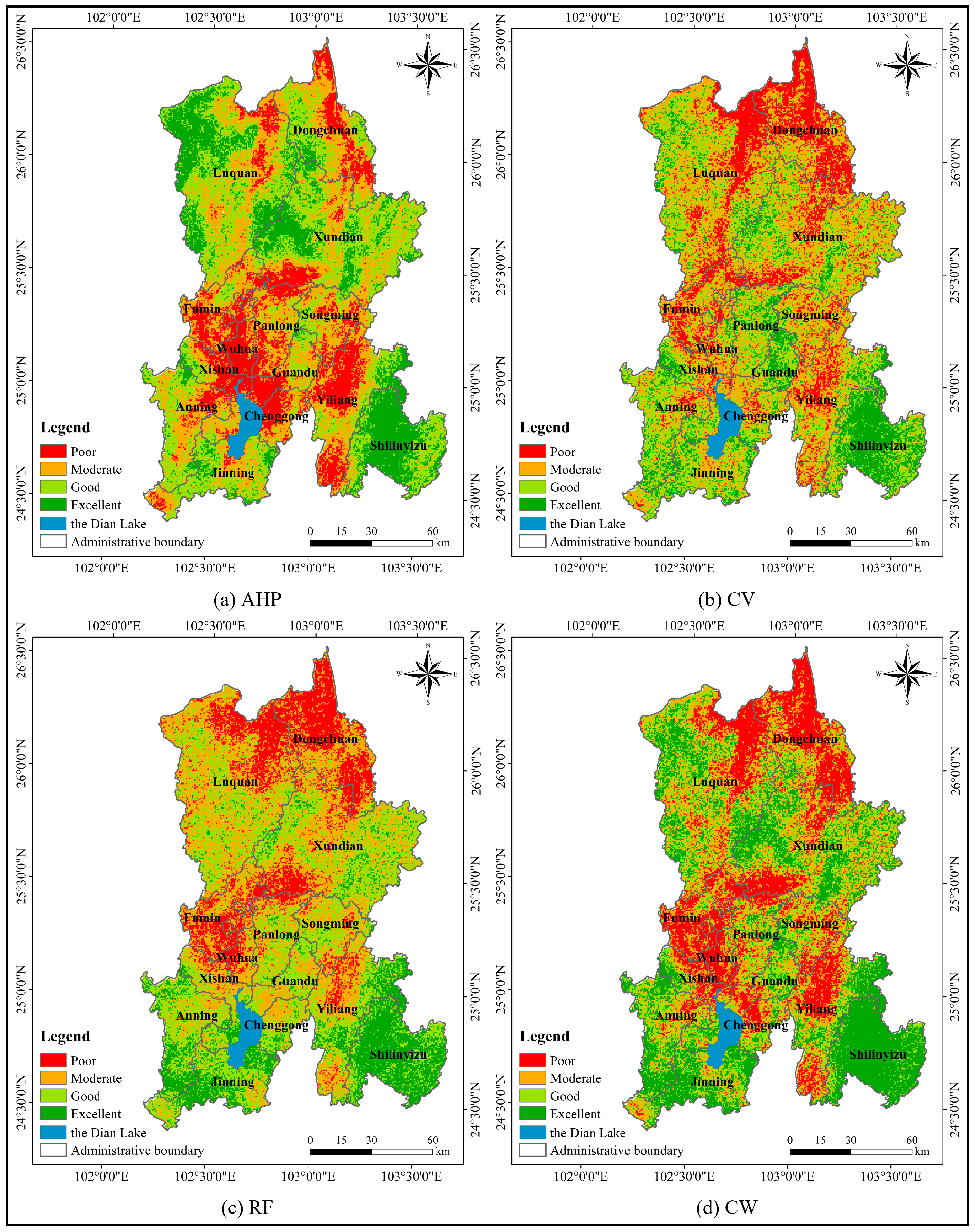
The data from each indicator layer and the criterion layer were calculated using Equation (12). Based on the natural breaks classification standard, the values were divided into four categories, Excellent, Good, Moderate, and Poor, resulting in the spatial distribution of Kunming City’s EGECC under different weighting schemes (Figure 3).

An analysis of the spatial distribution of the EGECC (Figure 3) and the corresponding area proportions (

Table 4. Area and proportion of EGECC classes in Kunming under different weighting methods.

	Excellent		Good		Moderate		Poor
	Area (km2)	Proportion	Area (km2)	Proportion	Area (km2)	Proportion	Area (km2)	Proportion
AHP	3703.38	17.80%	7006.81	33.69%	6313.91	30.36%	3775.71	18.15%
CV	3080.61	14.81%	6831.85	32.85%	7079.86	34.04%	3807.48	18.31%
RF	3103.99	14.92%	7533.88	36.22%	6728.84	32.35%	3433.09	16.51%
CW	5694.42	27.38%	5447.87	26.19%	4838.25	23.26%	4819.26	23.17%

) under different weighting methods yields the following observations:

(1)

EGECC pattern derived from the AHP weighting method:

Under the AHP weighting method, the four EGECC classes have relatively uneven area proportions, ranging from 17.80% to 33.69%. The Good and Moderate classes dominate, accounting for 33.69% and 30.36% of the total valid evaluation area, respectively. Poor areas are concentrated mainly in the five urban districts (Wuhua, Panlong, Guandu, Xishan, and Chenggong) and along the margins of certain counties (e.g., Fumin, Yiliang, northeastern Dongchuan, and northeastern Luquan). In contrast, higher-capacity areas are located primarily in western Luquan, central–western Xundian, and Shilin County. The remaining areas display strip-like distributions of “Good” and “Moderate” levels.

(2)

EGECC pattern derived from the CV weighting method:

Compared with the AHP results, the CV weighting method produces a slightly higher proportion of the Moderate class, which accounts for 34.04%, followed by the Good class at 32.85%. The Excellent and Poor classes account for 14.81% and 18.31%, respectively. Poor areas are concentrated in Fumin, Songming, Yiliang, and the main urban areas near Dianchi Lake. Superior areas are mainly found in Shilin County and Guandu District, whereas the rest of the region is characterized by patch-like distributions of “Good” and “Moderate” levels.

(3)

EGECC pattern derived from the RF weighting method:

The distribution pattern resembles that of the AHP results, with the Good class having the highest proportion at 36.22%, followed by the Moderate class at 32.35%. The Excellent and Poor classes account for 14.92% and 16.51%, respectively. Poor areas are located in Fumin, Wuhua, Yiliang, and the edges of Dongchuan, while higher-capacity areas are concentrated in Shilin County, Jinning District, and Anning City. Other regions generally show patch-like distributions of “Good” and “Moderate” levels.

(4)

EGECC pattern derived from the CW method:

The CW method results show a more balanced distribution among the four EGECC classes, with the Excellent class accounting for the largest proportion at 27.38%, followed by the Good, Moderate, and Poor classes at 26.19%, 23.26%, and 23.17%, respectively. Poor areas are distributed in Wuhua, Fumin, and Yiliang, whereas superior areas are concentrated in Shilin County, Jinning District, and Anning City. The remaining regions exhibit clustered patches of “Good” and “Moderate” levels.

In summary, the weighting method clearly influences the area proportions of the four EGECC classes. The Excellent class shows the lowest proportion under the CV method and the highest under the CW method, with a difference of 12.57 percentage points. The Good class ranges from 26.19% under the CW method to 36.22% under the RF method, with a difference of 10.03 percentage points. The Moderate class also varies notably, from 23.26% under the CW method to 34.04% under the CV method. In contrast, the Poor class shows a relatively smaller range, from 16.51% under the RF method to 23.17% under the CW method. These results indicate that different weighting methods affect not only the spatial pattern of EGECC but also the proportional allocation of areas among different carrying-capacity classes.

4.2. Evaluation of the EGECC in Counties (Districts)

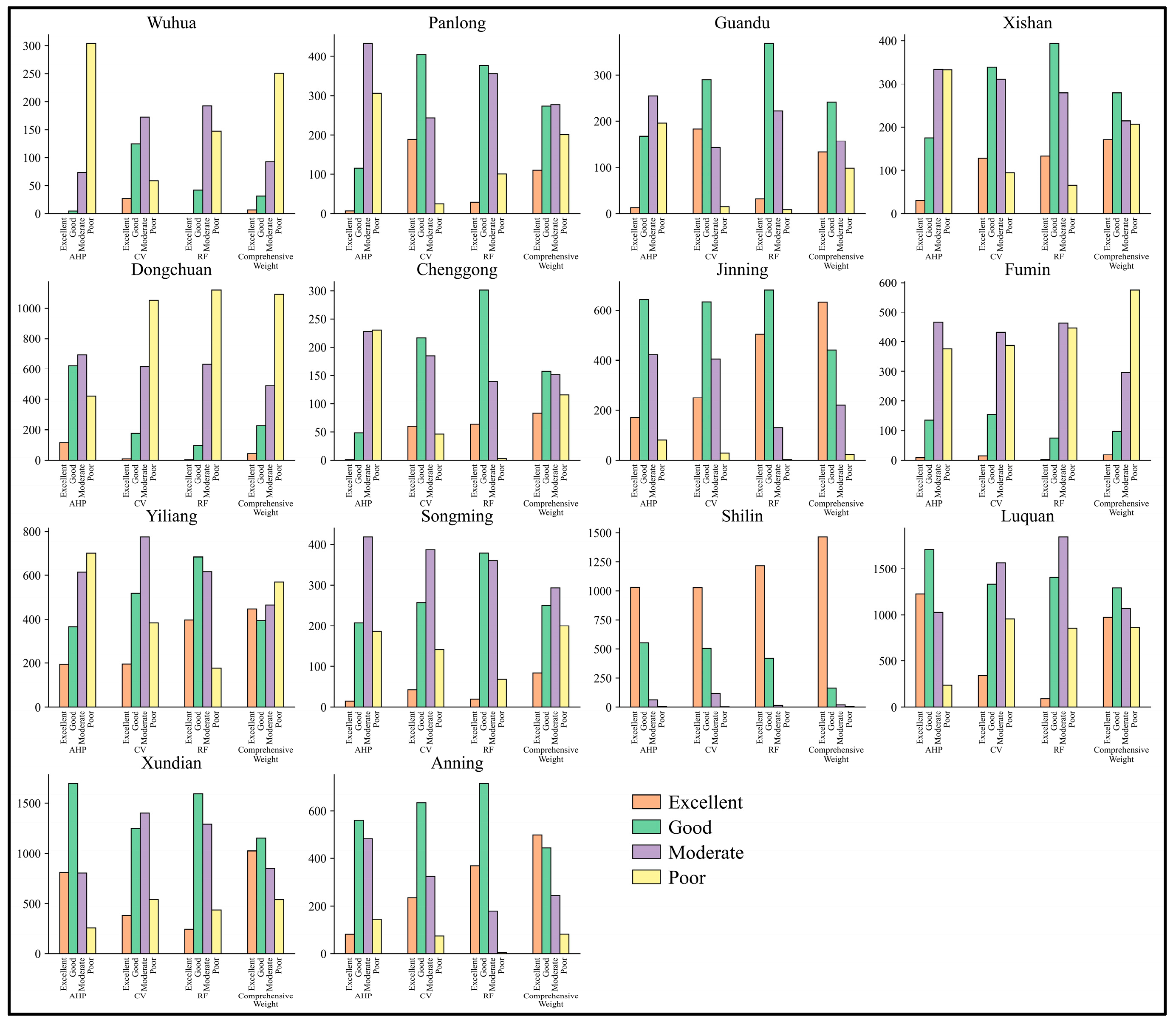
By statistically analyzing the areas corresponding to different EGECC levels in each county (district) of Kunming City (Figure 4) and calculating the average carrying capacity level (Figure 5), the evaluation results under different weighting methods can be compared. The analysis yields the following observations.

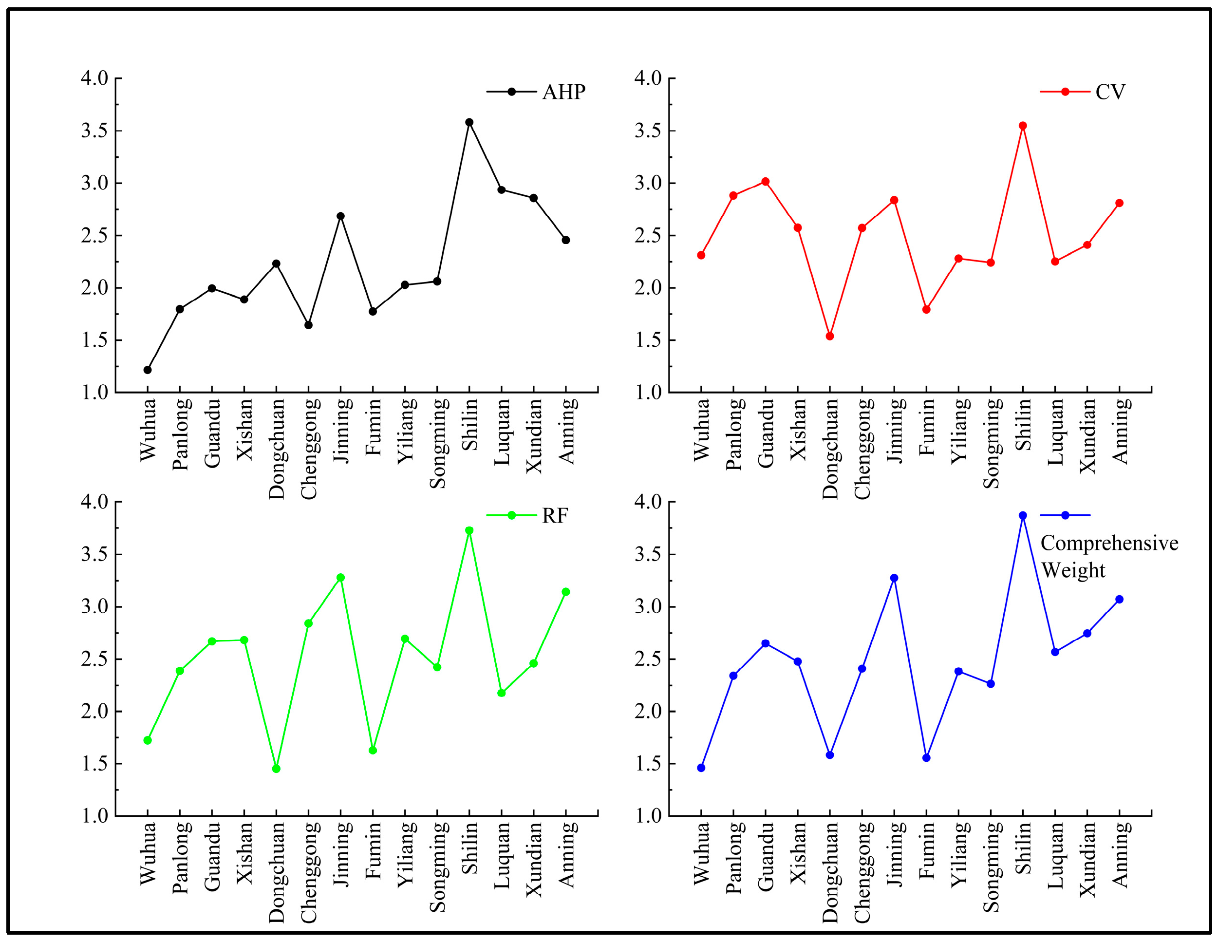
Shilin County has the highest average EGECC level under all four weighting methods. In contrast, Dongchuan District has the lowest evaluation values under the CV and RF methods, and Wuhua District has the lowest average EGECC level under the AHP and CW methods. Although the overall distribution trends of the level averages across methods are generally consistent, the AHP method shows slight differences due to subjective factors in weight determination. This implies that incorporating objective weight considerations when multiple evaluation methods are used may increase the robustness of the assessment.

Across different weighting methods, the indicator weights for Wuhua District suggest that the CW method is most influenced by the AHP results, resulting in relatively similar area proportions across levels. In contrast, Panlong District shows variations in area proportions across levels under different weighting methods, with the impacts of the AHP, CV, and RF methods being comparable to those of the CW method. A similar pattern is observed in Guandu District, Yiliang County, Luquan County, and Xundian County. In Xishan District, the area proportion trends across levels are consistent between the CV and RF methods, whereas in Chenggong District the pattern is similar. Dongchuan District exhibits broadly consistent trends across the CV, RF, and CW methods. In Jinning District, the area proportion trends remain similar under the AHP and CV methods, and a comparable pattern is observed in Anning City. Fumin County shows relatively consistent area proportions across the AHP, CV, and RF methods, whereas Songming County shows similar trends under the AHP and CV methods, with alignment also observed under the CW method. Finally, Shilin County consistently maintains the highest proportion of “Excellent”-level areas across all four weighting methods.

This comparative analysis illustrates the varying effects of different weighting methods on the spatial distribution and area proportions of EGECC levels across the counties and districts of Kunming City.

4.3. Spatial Autocorrelation Analysis

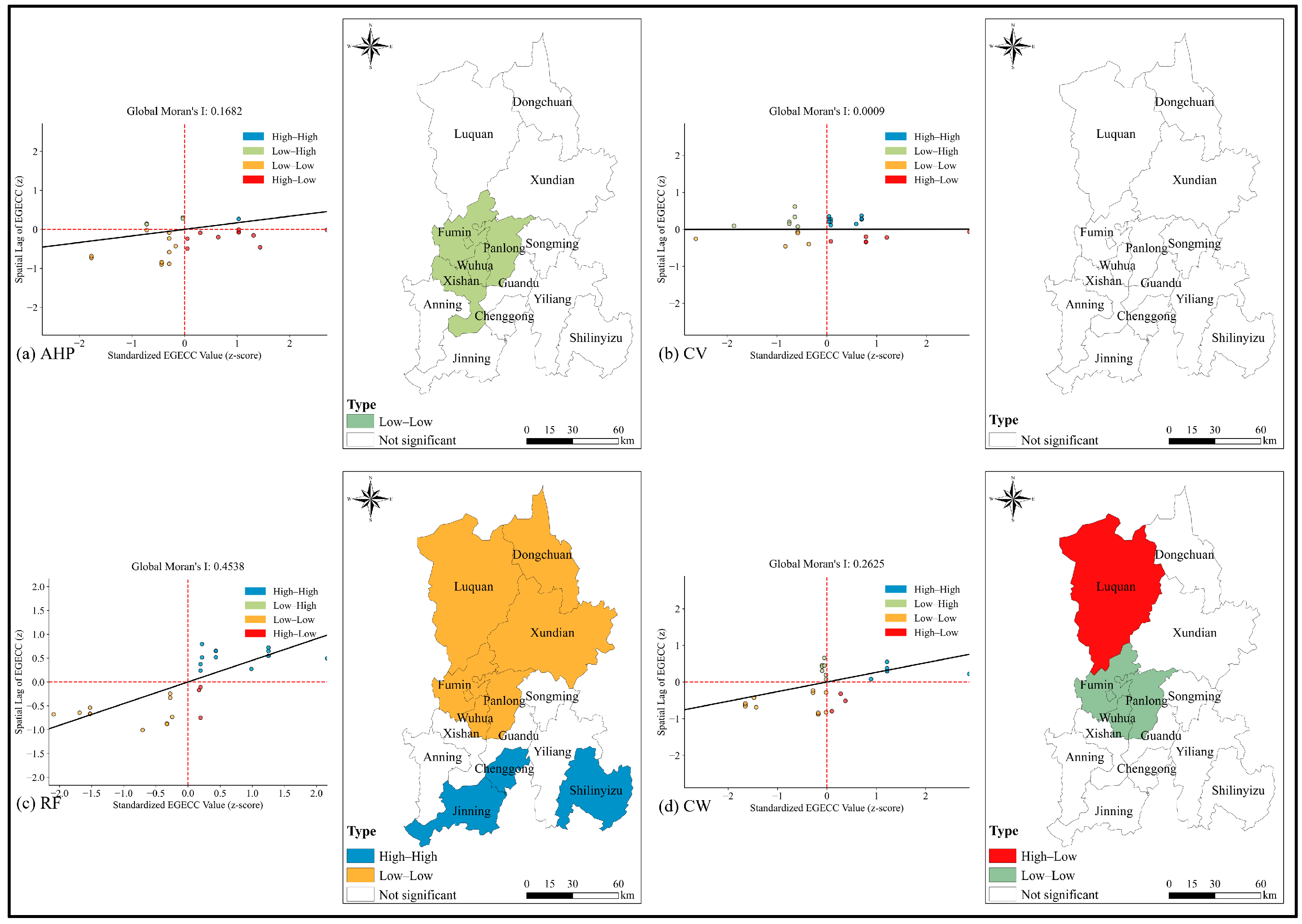
At the county level, Global Moran’s I and Local Moran’s I analyses were conducted on the mean EGECC values of each county (or district). Therefore, the spatial autocorrelation results reflect regional-level clustering rather than fine-scale raster-level spatial dependence. The global Moran scatterplot derived from the RF method indicates relatively strong positive spatial autocorrelation, whereas the CV method produces an essentially random spatial pattern (Figure 6). Under the AHP method, Global Moran’s I was 0.1682, suggesting modest positive spatial autocorrelation. At the local level, only Fumin, Wuhua, Xishan, and Panlong showed significant clustering in the Low–Low (LL) category, suggesting that these areas are characterized by relatively low, spatially clustered EGECC values, whereas the remaining regions did not exhibit statistically significant autocorrelation. In contrast, the CV method yielded a near-zero Global Moran’s I of 0.0009, implying that at the county scale, there is no discernible spatial clustering when only objective data variability is considered; under this scheme, no county demonstrated significant clustering. The RF method produced a higher Global Moran’s I of 0.4538, indicating stronger overall spatial autocorrelation. In this case, counties such as Fumin, Wuhua, Panlong, Luquan, Dongchuan, and Xundian were identified as Low–Low clusters, whereas Jinning, Chenggong, and Shilin formed High–High (HH) clusters, reflecting areas of consistently higher EGECC values. The CW method resulted in a Global Moran’s I of 0.2625, with Fumin, Wuhua, and Panlong classified as Low–Low clusters and Luquan emerging as a High–Low (HL) outlier. This suggests that while most adjacent counties have similarly low EGECC values, Luquan deviates by showing relatively higher values in this local context.

Overall, the differences among the weighting methods highlight the sensitivity of spatial autocorrelation results to the approach used to determine weights. In particular, the lower Global Moran’s I under the CV method may be related to data smoothing effects from purely objective weighting, whereas the RF method, by accounting for nonlinear relationships, reveals stronger spatial clustering. The CW method, which integrates subjective and objective assessments, produces intermediate outcomes that reflect both inherent spatial patterns and expert-informed adjustments.

4.4. Driving Mechanisms of Spatial Heterogeneity

GeoDetector analysis was used to further explain the spatial heterogeneity of EGECC. Factor detection identifies the explanatory power of individual indicators, interaction detection examines whether pairs of factors jointly enhance or weaken explanatory power, and risk detection compares EGECC differences among the classified intervals of each factor. These three modules provide complementary information on dominant drivers, nonlinear interactions, and favorable or unfavorable factor intervals.

4.4.1. Factor Detection

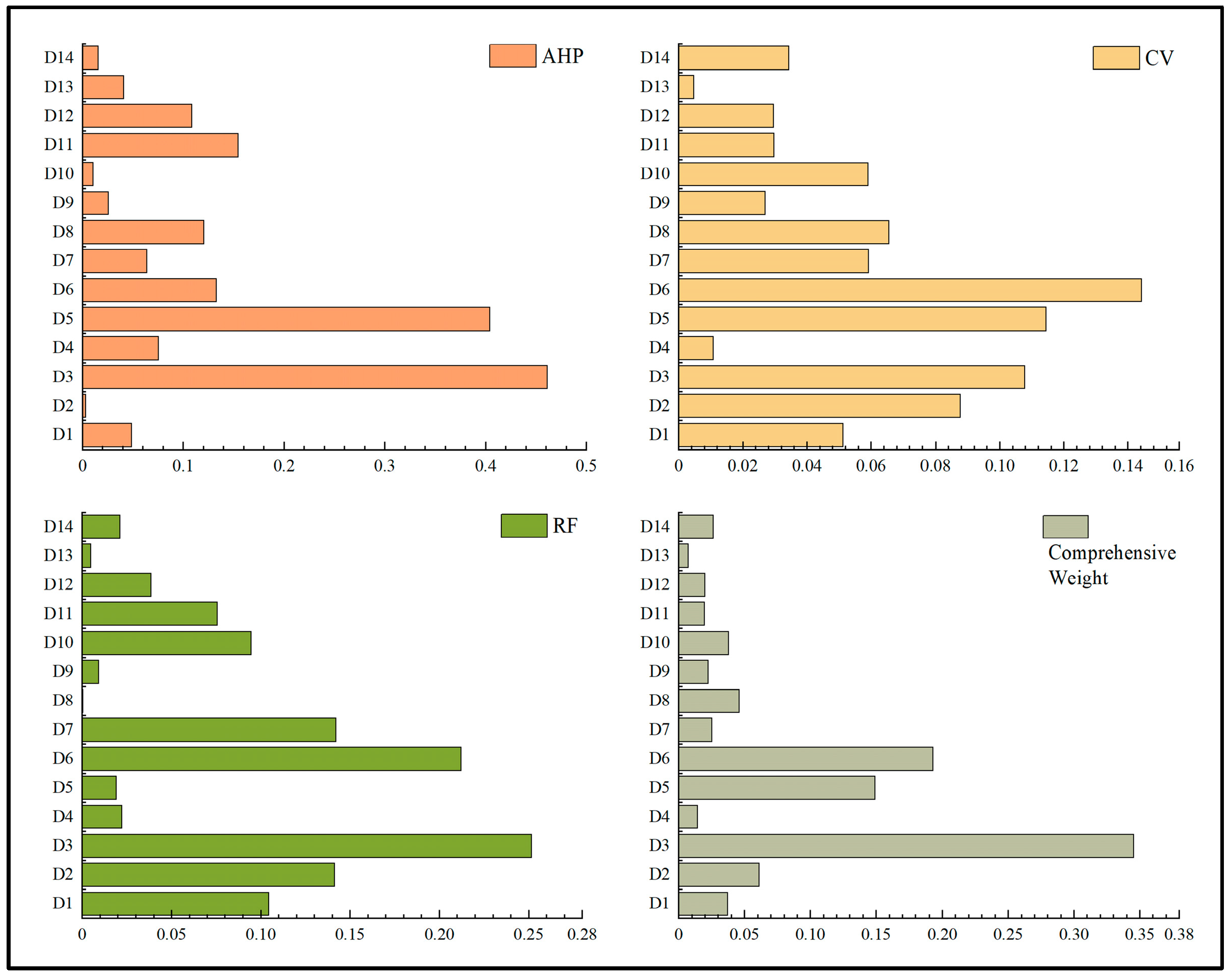
The spatial heterogeneity of the EGECC is jointly shaped by natural constraints and human activities, with strong interaction indicating nonlinear coupling. To assess the contribution of each driving factor to the EGECC, the factor detection module of the geographic detector was applied to calculate the q value, which represents the explanatory power of each indicator for variations in the carrying capacity under different weighting methods (Figure 7). As shown in Figure 7, the AHP, RF, and CW methods all suggest that hazard-point density has the highest explanatory power for eco-geological environmental carrying capacity, with q values of 0.4610, 0.2517, and 0.3453, respectively, indicating that it is a major driving factor. In contrast, the CV method yields a q value of 0.1443 for average annual precipitation, suggesting that precipitation is the primary explanatory factor in this case. Additionally, slope, arable land conditions, and the NDBI have relatively weak explanatory power under the AHP method but stronger effects under the CV and RF methods. Moreover, distance to water systems and road density have lower explanatory power in the RF results, whereas they appear to be more influential under the other three methods.

In summary, across the four weighting methods, elevation, hazard-point density, distance to faults, average annual temperature, average annual precipitation, population density, and GDP density emerged as common primary explanatory factors. In contrast, engineering geological rock formations, vegetation coverage, road density, and the NDBI served as common secondary explanatory factors.

4.4.2. Interaction Detection

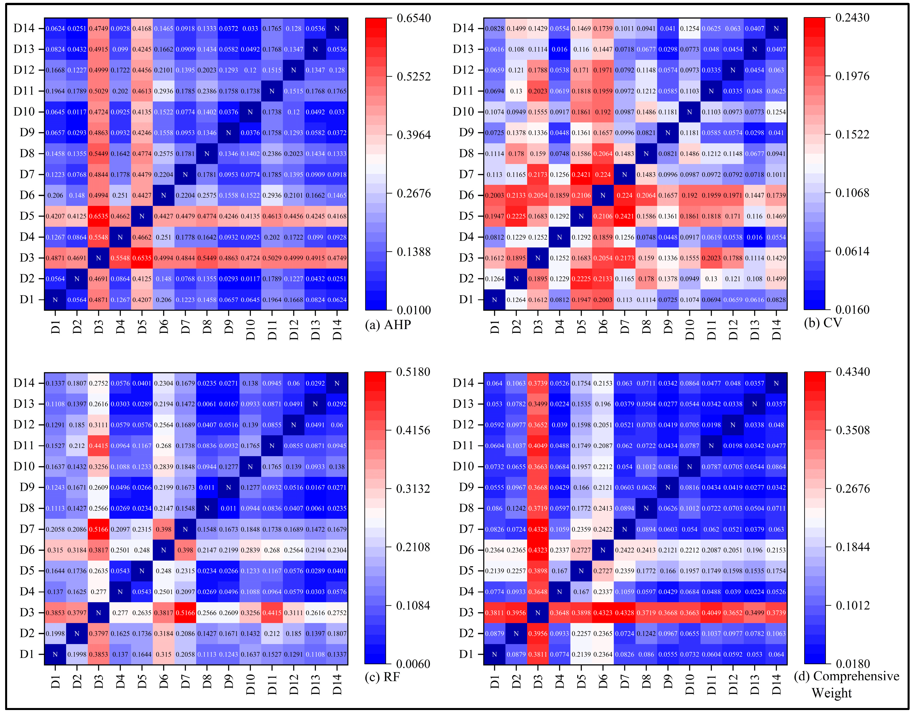
According to the five types of interactions defined by the geographic detector, the combined explanatory power of any two driving factors on variations in the EGECC was examined (Figure 8). As shown in Figure 8, across the four weighting methods, the interaction between hazard-point density and other factors consistently ranks among the highest, with its q value remaining at the top. Under the AHP and CW methods, the explanatory power is relatively strong, with q values exceeding 0.47 and 0.34, respectively. Additionally, the interactions between distance to faults and other factors are relatively strong under the AHP and CV methods, with q values above 0.41 and 0.11, respectively. The interactions between slope and hazard-point density, distance to faults, and average annual precipitation are also stronger than the interactions between slope and other factors. In contrast, the interactions among average annual temperature, distance to water systems, vegetation coverage, arable land conditions, population density, GDP density, road density, and the building index are weaker. These results suggest that interactions among key geological and ecological factors increase the explanatory power for variations in regional EGECC, emphasizing the importance of geological environmental influences in shaping spatial heterogeneity.

4.4.3. Risk Detection

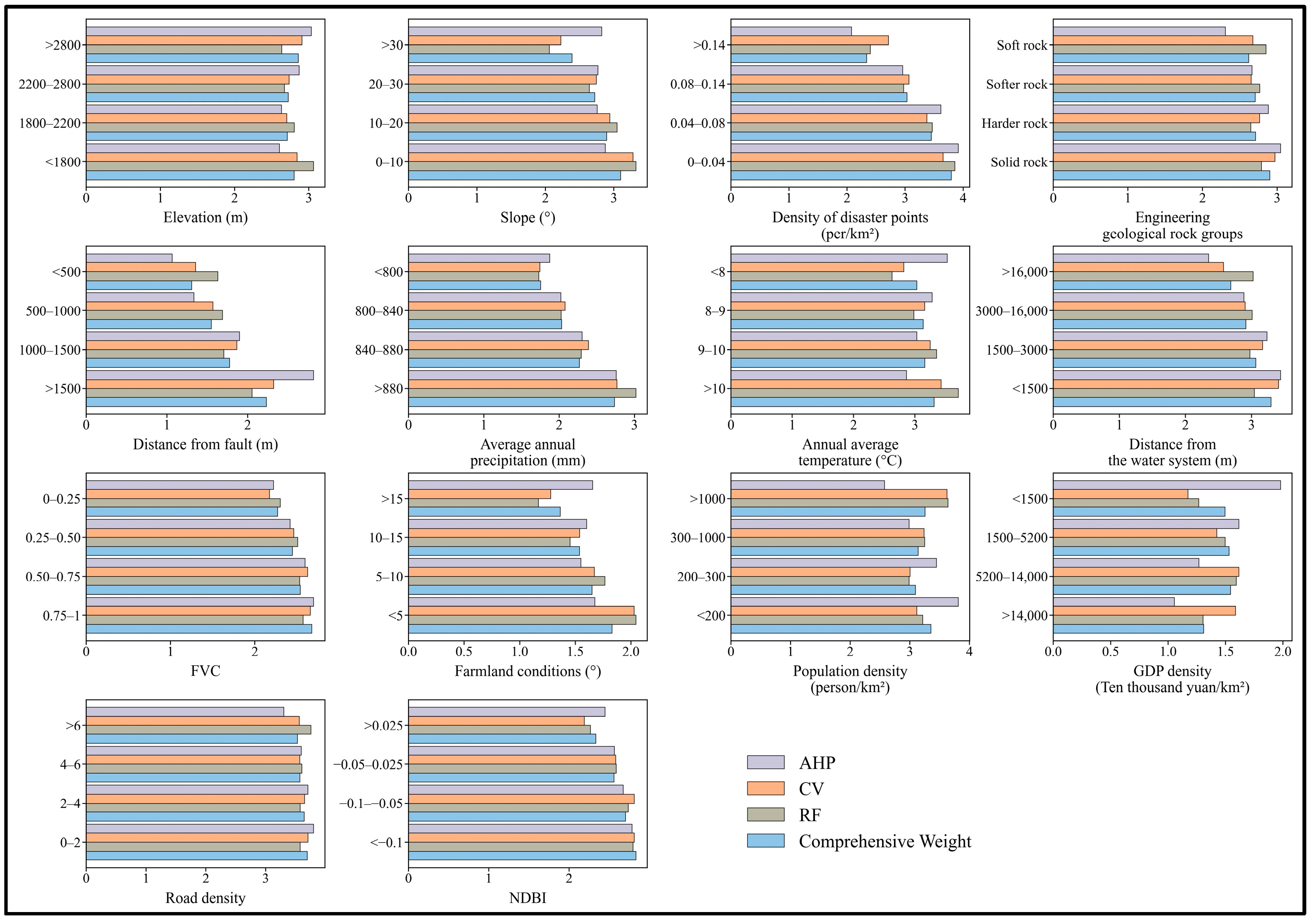
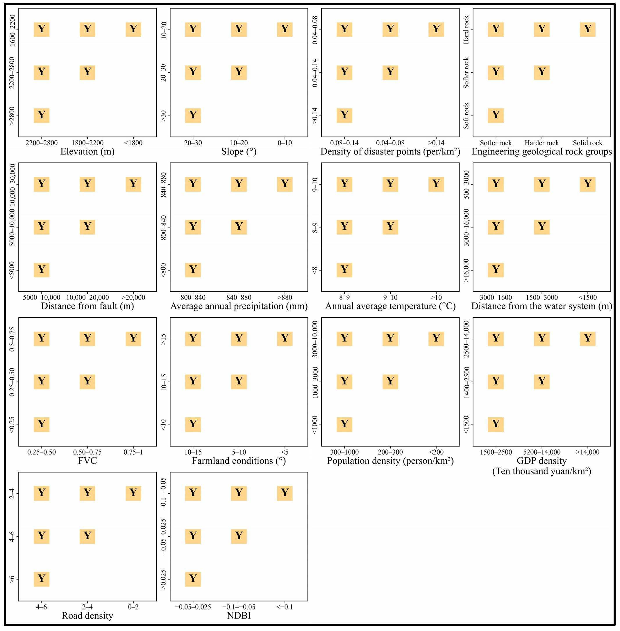
Risk detection was employed to evaluate the statistical significance of different indicator intervals in influencing EGECC, thereby helping to identify relatively favorable functional zones. As illustrated in Figure 9, the variation in the EGECC across the classified intervals of key indicators was analyzed under different weighting strategies. Across all four weighting approaches, the optimal intervals of most indicators generally aligned with their ecological attributes. For example, slope values of 0–10°, disaster point densities ranging from 0 to 0.04 events/km², fractional vegetation cover (FVC) values between 0.75 and 1, and NDBI values below −0.1 were commonly associated with higher EGECC levels. However, discrepancies were observed for some indicators. For instance, the AHP-based model identified low GDP-density zones as optimal regions, contradicting the expected positive relationship between GDP density and carrying capacity. This may reflect the subjectivity inherent in expert-driven weighting schemes. Although the random forest model effectively identified influential variables, its sensitivity to extreme values occasionally led to the misclassification of optimal intervals for indicators such as elevation and population density.

The risk detection matrix (Figure 10) further quantified the significance of the indicator intervals in relation to the EGECC levels. While most classified intervals exhibited statistically significant associations with carrying capacity, some methods tended to either overestimate or underestimate the influence of marginal intervals. Overall, the composite weighting method, which integrates subjective, objective, and data-driven perspectives, provided relatively greater stability and interpretability in interval classification, suggesting improved consistency and adaptability for spatial risk assessment.

4.5. External Validation

To externally examine the reliability of the EGECC classification results, geological hazard points were overlaid with the EGECC maps derived from the four weighting methods. The number of hazard points within each EGECC class was counted, and hazard-point density was further calculated to account for differences in class area (

Table 5. Distribution of geological hazard points across EGECC classes under different weighting methods.

	AHP		CV		RF		CW
	Number of Hazard Points	Hazard-Point Density (Points/km2)	Number of Hazard Points	Hazard-Point Density (Points/km2)	Number of Hazard Points	Hazard-Point Density (Points/km2)	Number of Hazard Points	Hazard-Point Density (Points/km2)
Poor	541	0.14	425	0.11	390	0.11	390	0.08
Moderate	415	0.07	456	0.06	469	0.07	469	0.10
Good	237	0.03	296	0.04	336	0.04	336	0.06
Excellent	65	0.02	81	0.03	63	0.02	63	0.01

). Because areas with lower carrying capacity are expected to have weaker geological stability and higher hazard susceptibility, a reasonable EGECC classification should show higher hazard-point density in the Poor or Moderate classes and lower hazard-point density in the Good or Excellent classes.

The external validation results reveal that geological hazard points are generally more concentrated in lower EGECC classes. Under the AHP, CV, and RF methods, hazard-point density decreases consistently from the Poor class to the Excellent class, indicating a generally consistent relationship between lower carrying capacity and higher geological hazard occurrence. For the CW method, the highest hazard-point density occurs in the Moderate class, followed by the Poor class, while the Excellent class has the lowest density. This suggests that the CW-based classification is not strictly monotonic across all classes, but it still effectively distinguishes lower-capacity areas from high-capacity areas. Overall, the validation results provide external support for the consistency of the EGECC classification, as areas with Poor or Moderate carrying capacity generally have higher geological hazard-point density than Good and Excellent areas.

5. Discussion

5.1. EGECC Analysis

Based on the evaluation results across different weighting methods, the EGECC of Kunming City shows clear spatial heterogeneity, with Good and Moderate classes dominating under the AHP, CV, and RF methods, whereas the CW method produces a more balanced distribution across the four classes. In particular, higher EGECC values are mainly observed in the southeastern and southwestern areas, whereas lower values are concentrated in the northern mountainous areas and highly urbanized central districts, which is broadly consistent with previous findings on ecological environmental differentiation in Kunming [60]. The lower carrying capacity in these areas is largely due to the regional geological background and intensive human disturbance, including the distribution of hazard points, engineering geological rock formations, active faults, and dense construction activities. These areas are more susceptible to natural disaster risks [61] and have relatively fragile ecological environments, which contribute to their lower EGECC.

The spatial pattern identified in this study is generally consistent with that reported in previous studies on ecological quality and geological hazard risk in Kunming and surrounding mountainous areas. Previous research has shown that the central urban area of Kunming and areas with intensive construction activities tend to experience greater ecological pressure, while regions with better vegetation conditions and lower disturbance intensity usually have better ecological environmental quality. Similarly, studies on geological hazards in Dongchuan and other mountainous districts of Kunming have emphasized the influence of steep terrain, active faults, and concentrated hazard points on regional environmental stability. These findings support our conclusion that low-EGECC areas are mainly associated with dense anthropogenic activity, fragile geological settings, and relatively high hazard susceptibility.

To further explore these regional differences and their influencing factors, the average EGECC for each county (district) was calculated under the four weighting methods (

Table 6. Mean EGECC values of counties/districts averaged across the four weighting methods.

	Wuhua	Panlong	Guandu	Xishan	Dongchuan	Chenggong	Jinning
Mean	1.6782	2.3508	2.5826	2.4055	1.7016	2.3666	3.0203
	Fumin	Yiliang	Songming	Shilin	Luquan	Xudian	Anning
Mean	1.6874	2.3464	2.2470	3.6835	2.4824	2.6188	2.8703

). The analysis is as follows.

Shilin County, which has the highest EGECC in Kunming City, has an average carrying capacity value of 3.6835. In this area, the elevation is generally less than 2200 m, most slopes are less than 10°, hazard points are sparse, geological structural activity is limited, and engineering geological rock formations are composed mainly of hard rocks. These conditions are associated with relatively stable geological structures, supporting higher geological environmental carrying capacity and contributing to a higher overall EGECC score. The variations in the weighting calculation methods have little effect on identifying Shilin County as the area with the highest carrying capacity.

Jinning District, Anning City, Xundian County, and Guandu District have moderately high EGECC values, ranging between 2.5 and 3. Luquan County, Xishan District, Chenggong District, and Panlong District have moderately low carrying capacities, ranging from 2.3 to 2.5. Although these areas have favorable conditions for economic development, their carrying capacity remains moderate, suggesting potential for improvement.

Songming County, Dongchuan District, Fumin County, and Yiliang County are strongly influenced by fault zones, leading to folded and faulted structures, increased hazard-point densities, average annual precipitation below 880 mm, and GDP densities under 15 million yuan/km². Combined with anthropogenic activities, these factors place additional pressure on the eco-geological environment, resulting in lower carrying capacity. Wuhua District, as the economic center of Kunming, has a GDP density exceeding 140 million yuan/km² and a high building density. Despite notable urbanization and economic growth, its average annual precipitation is less than 840 mm, and the population density exceeds 1000 persons/km². These factors contribute to Wuhua District having the lowest average EGECC of 1.6782.

5.2. Comparison of Different Weighting Methods

5.2.1. Correlation Coefficient

The Pearson, Spearman, and Kendall correlation coefficients between each pair of the four weighting methods were calculated, and the average correlation of each method with the others was evaluated. Among these, the Pearson correlation coefficient indicates whether the weighting methods yield similar absolute-value relationships across regions—for example, whether high-carrying-capacity areas show consistent absolute values under both methods. The Spearman correlation coefficient is used to determine whether the weighting methods yield consistent trends in the spatial distribution of the carrying capacity, i.e., whether the rankings from highest to lowest are similar. The Kendall correlation coefficient provides a stricter test of ranking consistency, emphasizing whether the direction of ranking changes is aligned. A higher average correlation value indicates that the method produces results that are more similar to those of the other methods, suggesting greater stability. An analysis of the data in

Table 7. Average correlation of EGECC based on different weighting methods.

	Mean Pearson Correlation	Mean Spearman Correlation	Mean Kendall Correlation
AHP	0.7161	0.6964	0.5121
CV	0.8149	0.7995	0.6164
RF	0.7620	0.7453	0.5644
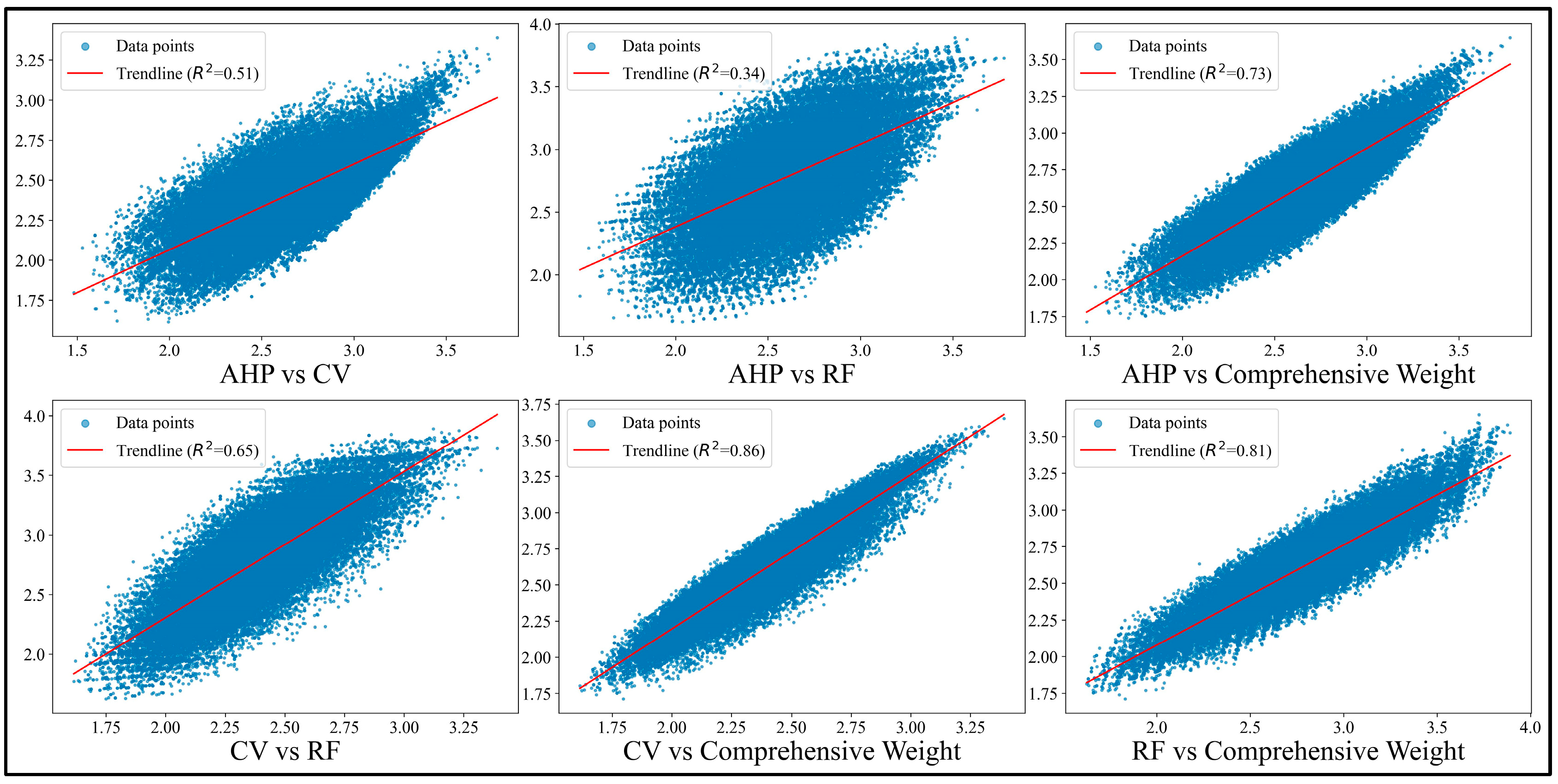
CW	0.8934	0.8831	0.7042

reveals that, among the four methods, the combined weighting method achieved the highest Pearson, Spearman, and Kendall correlation coefficients. The R² values obtained from comparisons between the combined weighting method and the other methods were above 0.7 (Figure 11). In summary, the results indicate relatively strong linear correlations across the methods, and the combined weighting method demonstrates closer alignment with the others, making it a useful reference for comprehensive evaluation.

5.2.2. Consistency of Overlapping Levels Across Regions

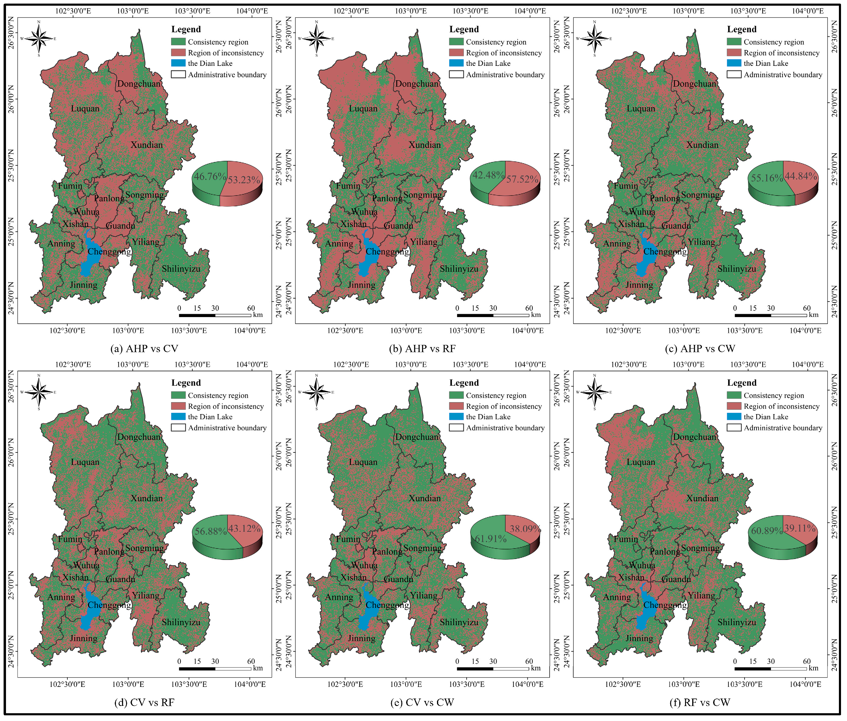
A pixel-by-pixel comparison of the EGECC layers obtained from any two weighting methods identifies regions of agreement and disagreement (Figure 12). Compared with the other three methods, the CW method produced a relatively higher proportion of consistent regions, with all the values exceeding 55%, whereas the consistency among the remaining three methods was lower. This pattern may be related to the integrative nature of the CW method, which combines AHP-, CV-, and RF-derived weights and reduces the dependence on a single weighting logic. However, this consistency should be interpreted as internal agreement among different weighting results rather than direct evidence of absolute accuracy. Therefore, the CW method can be regarded as a balanced integration scheme under the available-data condition, but its reliability still requires interpretation together with external validation and sensitivity analysis. In contrast, the lower consistency among the AHP, CV, and RF methods may be attributed to several factors. First, the weighting logic of these methods differs substantially: the AHP method is based on expert judgment and may emphasize certain subjectively favored factors; the CV method relies solely on data variability, assigning higher weights to factors with greater variation; and the RF method derives weights from feature importance rankings based on AHP- and CV-derived classification results, making the results more dependent on the training targets and algorithmic outputs. Second, the methods have different sensitivities to specific indicators. Third, the complexity of regional eco-geological features may amplify differences in weight allocation across methods, thereby contributing to lower consistency.

5.3. Validation and Sensitivity Analysis

To further assess the stability of weighting methods under indicator perturbations, a sensitivity-based consistency analysis was conducted, followed by a regional agreement comparison across different weighting schemes. By comparing the classification results before and after indicator perturbations, the responsiveness of each method to fluctuations in the core variables and its spatial robustness were evaluated, thereby assessing its resilience and practical applicability. Three key indicators—disaster point density, fractional vegetation cover (FVC), and the normalized difference built-up index (NDBI)—were selected because of their strong influence on weight assignment. For each, the composite weight was artificially increased by 10% and 20%, respectively, while proportionally rescaling the remaining weights to maintain a normalized sum of 1. The evaluation results under perturbed and baseline conditions were compared using the kappa consistency coefficient to examine performance differences across weighting methods (

Table 8. Kappa consistency coefficients under key indicator perturbations across different weighting methods.

	D3+10%	D3+20%	D9+10%	D9+20%	D14+10%	D14+20%
AHP	0.5891	0.5817	0.5839	0.5750	0.5793	0.5648
CV	0.3474	0.3466	0.3411	0.3336	0.3382	0.3290
RF	0.4471	0.4393	0.4443	0.4428	0.4240	0.4005
CW	0.4122	0.4154	0.4036	0.3989	0.3954	0.3839

).

As shown in Table 8, under all six perturbation scenarios, the AHP method yields the highest average kappa value (0.581), suggesting relatively low sensitivity to weight fluctuations. This relative stability is likely due to the more uniform weight distribution of the AHP, which reduces the influence of adjustments to individual indicators. Although the random forest (RF) method is data-driven, its weight distribution is concentrated around a few dominant variables, making it less responsive to changes in non-core indicators. As a result, RF demonstrates moderate robustness, with an average kappa value of 0.442.

In contrast, both the coefficient of variation (CV) method and the composite weighting (CW) method produce lower kappa values under perturbation, suggesting higher sensitivity and more pronounced spatial classification shifts. Although the CW method benefits from integrating multiple weighting strategies, it also shows greater responsiveness when high-weight indicators are perturbed, reflecting its sensitivity to dominant-variable adjustments.

5.4. Limitations

Despite the integration of the AHP, CV, and RF methods and an improved linear efficacy coefficient method to enhance the rigor of EGECC assessment, this study has several limitations.

First, although combining multiple weighting techniques improves model adaptability and provides a more comprehensive characterization of indicators, the evaluation framework relies primarily on remote sensing imagery and statistical datasets, with limited incorporation of in situ observational data. For indicators with high spatial heterogeneity—such as disaster point density, engineering geological lithology, and the NDBI—the model may not fully capture localized variability, which could lead to discrepancies between estimated outcomes and actual eco-geological conditions. Although geological hazard points were used as an external consistency check and provided an independent reference for evaluating the EGECC classification results, this validation mainly reflects mainly consistency with geological hazard occurrence. More independent field-based observations, ecological degradation data, and long-term monitoring records are still needed to comprehensively validate the EGECC results.

Second, although the random forest algorithm is useful for identifying nonlinear relationships, its “black-box” nature constrains the interpretability of the weight assignment process, reducing transparency and traceability. In addition, the RF-derived weights in this study were trained using the AHP- and CV-derived classification results rather than independent ground-truth observations. Therefore, they should be interpreted as nonlinear correction weights embedded in the existing evaluation results rather than fully independent weights.

Third, the evaluation was conducted partly at the county/district level, and the results may be sensitive to the choice of spatial scale. The patterns identified at this resolution may not be consistent with those derived from finer (e.g., township or grid) or broader (e.g., provincial) scales. In particular, aggregating raster-based results to county- or district-level statistics may smooth local heterogeneity and affect the observed spatial patterns. Therefore, county- and district-level results should be interpreted as regional summaries, while fine-scale raster maps remain necessary for identifying local variations. Fourth, although the study integrated multiple weighting methods, the indicator system itself still involves subjective choices and is partly constrained by data availability. This may limit the universality of the framework. In addition, some indicators, such as temperature, precipitation, GDP density, and road density, may have nonlinear or threshold effects rather than strictly monotonic relationships with the EGECC. Although interval-based grading was used to reduce this simplification, future studies should consider optimal-range functions or distance-to-ideal methods to better represent non-monotonic indicator effects.

Fifth, while the composite weighting method shows promising adaptability in Kunming, its transferability to regions with different eco-geological contexts remains uncertain and requires further empirical testing. Moreover, the sensitivity analysis focused mainly on weight perturbations of selected key indicators and did not fully capture the uncertainty in the input indicator values or classification thresholds. Therefore, the sensitivity results should be interpreted as an assessment of weighting robustness rather than a comprehensive uncertainty analysis.

Finally, the analysis relies primarily on cross-sectional data, and limited consideration has been given to dynamic responses to rapidly changing anthropogenic activities or sudden geological hazards, which may influence carrying capacity in practice.

Future research should integrate higher-resolution ground-based measurements and dynamic monitoring data to conduct multi-scale, multi-source validation of model outputs. Such efforts would improve the empirical reliability, applicability, and generalizability of EGECC evaluations.

6. Conclusions

In this study, Kunming City was taken as the study area, and evaluation factors related to the geological, ecological, and socioeconomic environments were selected to construct an indicator system for assessing the EGECC. Four weighting methods—AHP, CV, RF, and CW—were applied to calculate indicator weights, and the evaluation results under different methods were compared. Based on these outcomes, the spatial autocorrelation of EGECC and its driving factors across different regions were further analyzed, leading to the following findings.

(1) The EGECC of Kunming City clearly shows spatial heterogeneity, with higher values distributed mainly in the southeastern and southwestern areas and lower values concentrated in the northern mountainous areas and highly urbanized central districts. The spatial distributions derived from the CV and RF methods are relatively similar, and those from the AHP and CW methods also exhibit comparable patterns.

(2) When average EGECC levels are compared, all the weighting methods indicate that Shilin County has the highest value. Under the CV and RF methods, Dongchuan District has the lowest value, whereas under the AHP and CW methods, Wuhua District has the lowest value.

(3) Global and local Moran’s I analyses across counties suggest that the RF-based results show stronger positive spatial autocorrelation and clearer clustering patterns. In contrast, the results of the CV method reveal an almost random distribution. The AHP and CW methods yield intermediate results between these two extremes.

(4) The results from the geographic detector model suggest that the combined effect of geological and environmental factors plays an important role in shaping Kunming City’s EGECC. The AHP, CV, and RF methods each provide useful but different weighting perspectives, although they also have limitations, such as the subjectivity of the AHP, the reliance of the CV on data variability, and the limited interpretability of RF. The CW method provides relatively balanced results by integrating expert-knowledge-based, data-dispersion-based, and nonlinear data-driven information; however, its reliability should be interpreted alongside the geological-hazard-point validation and weight-perturbation sensitivity analysis conducted in this study.

Nevertheless, the findings should be interpreted with caution, given the study’s reliance on remotely sensed and statistical data, as well as the methodological sensitivities discussed above. Geological hazard points were introduced as an external consistency check, and a sensitivity analysis was designed to evaluate the robustness of the weighting scheme by perturbing selected key indicator weights. Future research should incorporate higher-resolution field observations, multi-source dynamic monitoring data, and more comprehensive uncertainty analysis to further enhance the reliability and applicability of EGECC evaluations.