1. Introduction
Land degradation is a major threat to soil fertility [
1], agricultural productivity [
2], water quality [
3], and ecosystem stability worldwide [
4], with soil erosion by water representing one of its most important forms. It is especially critical in Mediterranean environments, where steep topography, intense seasonal rainfall, sparse vegetation cover during part of the year, and long-term agricultural use create favorable conditions for runoff generation and soil detachment [
5,
6,
7]. In these landscapes, erosion is not only a geomorphological process but also a major environmental and socio-economic issue because it reduces the productive capacity of soils and contributes to the progressive degradation of cultivated land [
8,
9]. Olive-growing areas are particularly relevant in this context, as they represent one of the dominant land uses in many Mediterranean regions and are often located on sloping terrain that is vulnerable to erosion [
7,
10].
The Mediterranean climate is characterized by a strong seasonal contrast, with dry summers and rainfall concentrated mainly in autumn and winter [
11]. Under these conditions, the erosive impact of rainfall is often intensified by the limited protective cover of the soil surface at the beginning of the rainy season. In many olive orchards, especially those managed conventionally, the soil between tree rows may remain bare or only partly covered for long periods, increasing its exposure to raindrop impact and overland flow [
12]. Repeated tillage, low organic matter content, and inadequate conservation practices may further increase soil susceptibility to erosion [
13,
14]. As a result, Mediterranean olive groves have frequently been identified as high-risk areas for soil degradation, sediment redistribution, and long-term decline in soil quality [
15].
Because soil erosion is controlled by the interaction of multiple factors, including rainfall, soil properties, slope, vegetation cover, and land management [
16], its assessment remains methodologically challenging [
17]. No single approach can fully capture all dimensions of the process. Direct field measurements provide valuable information on actual soil loss under real conditions, but they are often limited to small plots and specific time periods [
18]. Empirical models, on the other hand, make it possible to estimate erosion over larger areas and to explore its spatial distribution, although their reliability depends strongly on the quality of the input data and on local validation [
19]. In recent years, high-resolution topographic techniques such as Light Detection and Ranging (LiDAR) and photogrammetry have added a new dimension to erosion studies by allowing the detection of subtle changes in surface elevation and local redistribution patterns [
20]. These different approaches are therefore complementary rather than interchangeable.
The Revised Universal Soil Loss Equation (RUSLE) is an empirical model used to estimate average annual soil loss caused by water erosion based on rainfall erosivity, soil erodibility, topographic characteristics, land cover, and conservation practices [
21]. Due to its broad applicability and relatively simple parameterization, RUSLE has become one of the most widely used approaches for soil erosion estimation [
22], making it particularly suitable for comparison with field-based measurements in the present study. Its widespread use is related to its relatively simple structure, modest data requirements compared with more physically based models, and compatibility with Geographical Information Systems (GIS)-based spatial analysis [
23]. For this reason, RUSLE has been used extensively in watershed studies, agricultural landscapes, and erosion risk mapping applications. However, its use also requires caution. Since RUSLE is an empirical model, its predictions depend heavily on the representativeness and spatial accuracy of the input factors, and its application is more robust when supported by local information and field observations. Validation is therefore essential if model outputs are to be interpreted with confidence [
24].
At the same time, field experiments remain one of the most direct ways to quantify real soil loss from a defined area. Measurements obtained from monitored plots can provide useful evidence of temporal variability and event-driven erosion, particularly in cultivated systems where soil loss may occur in short pulses associated with rainfall episodes [
18]. Such data are particularly valuable because they offer an empirical basis against which model results can be compared. Nevertheless, field measurements alone cannot describe the spatial distribution of erosion beyond the monitored plot, nor can they easily reveal how sediment is redistributed across the surface [
25]. This limitation has encouraged the integration of field observations with spatial models and terrain-based techniques.
In this context, LiDAR-derived digital elevation models (DEMs) and DEM of Difference (DoD) analysis provide an additional tool for investigating soil surface dynamics at very fine scales. By comparing elevation models acquired at different times, DoD analysis can identify areas of local surface lowering and raising, thereby helping to describe short-term terrain change and soil redistribution [
26]. While this method does not necessarily measure soil loss directly, it is particularly useful for visualizing surface behavior and the movement of material within small experimental plots. As such, it can complement both direct field measurements and model-based predictions by adding information on local microtopographic change.
The present study was developed within this broader methodological context and aimed to assess soil erosion in a Mediterranean olive-growing sub-catchment in southwestern Greece using a combination of approaches. More specifically, the study integrates (i) direct field measurements of soil loss from an experimental subplot, (ii) spatial estimation of soil erosion using the RUSLE model, and (iii) LiDAR- and DoD-based analysis of short-term surface elevation changes. The decision to focus on a small, well-defined sub-catchment was made to improve the spatial reliability of the RUSLE application and to allow direct comparison between model outputs and field observations at the location of the experimental plot. This design also makes it possible to examine how different methods perform when applied to the same erosion-prone environment.
The study, therefore, aims not only to estimate soil erosion but also to compare three different assessment approaches within the same sloping Mediterranean olive orchard, where erosion is strongly event-driven. The results indicate that runoff plots provide direct measurements of soil loss at the event scale, RUSLE yields satisfactory estimates when supported by local calibration data, and LiDAR-DoD contributes primarily to the spatial interpretation of surface change and sediment redistribution. The main contribution of the study thus lies not in the individual application of these methods, but in their combined evaluation within the same agroecosystem, highlighting how their complementarity can support a more complete understanding of erosion processes.
2. Materials and Methods
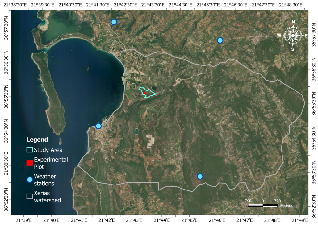
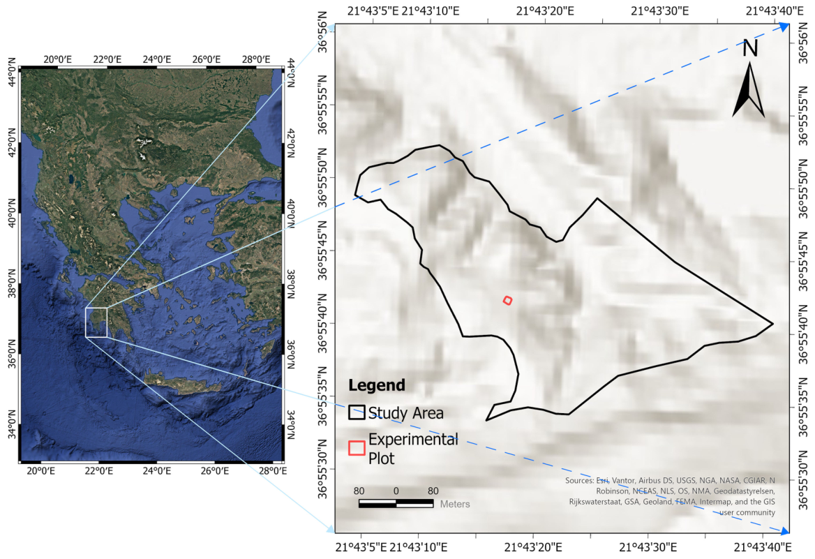
The study was carried out in a sub-catchment (0.221 km
2) of the Xerias River watershed (about 60 km
2), near the coastal area of Navarino gulf in Pylos-Nestor Municipality of Messenia, southwestern Greece (
Figure 1). Although the broader Xerias watershed covers a much larger area, the present analysis focused on a smaller section that was selected according to local topography which defines a clear and practical boundary for modelling purposes. This smaller unit was considered appropriate for the application of the RUSLE model, since it includes the experimental plots used in field study and represents the terrain conditions most relevant to the objectives of this work.
The landscape is typical of Mediterranean environments, with gentle to moderately sloping terrain, small drainage pathways, and agricultural land mixed with patches of natural vegetation. The dominant land use in the area is olive cultivation, accompanied by shrubland and scattered woodland vegetation. Soils are mainly calcareous Mediterranean soils, generally ranging from loam to clay loam [
27], and they have a moderate to relatively high susceptibility to erosion, especially where vegetation cover is limited. In addition, soil samples from the experimental field plot were analyzed in the beginning of the experiment for selected chemical and physical properties, including organic matter content [
28] and texture [
29]. Soil texture was classified according to the USDA soil texture triangle [
30].
The climate of the region is Mediterranean, with precipitation concentrated mainly in the wet season from autumn to spring, while summers are hot and dry [
31,
32]. Average annual precipitation during the 2016–2025 reference period was 806 mm, according to the local weather stations network. Under these conditions, soil loss is strongly influenced by seasonal rainfall intensity, slope, land cover, and management practices [
14]. The selected sub-catchment is a representative and well-defined area for investigating erosion processes at the local scale.
2.1. Field Monitoring of Runoff and Sediment
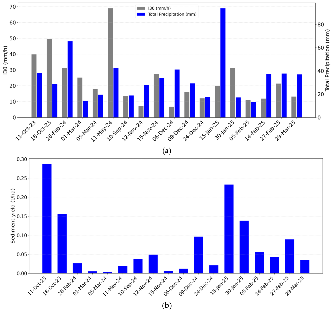
To anchor the modelling in empirical evidence under local orchard conditions, we used runoff and sediment data from a field experiment during October 2023–March 2025. More specifically, the experiment employed bounded runoff plots that route surface runoff and associated sediment to a collector and storage tanks, enabling event-scale quantification of runoff volume and sediment yield. Such plots are widely used in Mediterranean olive systems to measure gross soil loss and compare management practices, although known scale and border effects should be considered when interpreting results [
7].
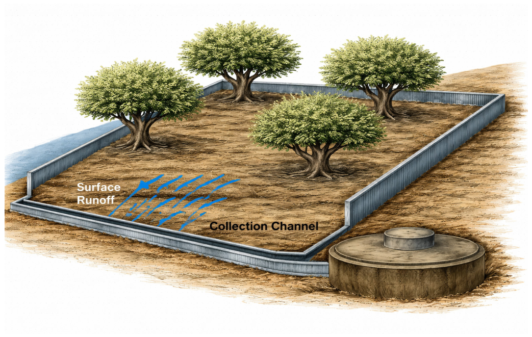
A randomized block design was used in the experiment, consisting of nine plots (10 m × 10 m) established on a representative hillslope within an olive grove. Three soil management treatments were evaluated, each with three replicates: herbicide treatment, cover cropping, and mowing of natural vegetation. In the present study, we report and analyze data from one plot corresponding to the herbicide treatment (one of the nine plots). This plot was selected because it was the only replicate within the herbicide treatment equipped with a surface runoff collection system, due to the high cost and complexity of the installation, which limited its implementation to one plot per treatment. In addition, the herbicide-treated plot belongs to the olive grove land-cover class considered in the assignment of the cover-management factor (C), while it was essential for the DoD analysis because reduced vegetation improved LiDAR surface detection. The plot was located on a slope segment with a mean gradient of ~16% and was equipped at its downslope boundary with (a) a collection channel/trough spanning the plot width and (b) a sealed storage tank positioned downslope to retain runoff and sediment from each rainfall event (
Figure 2). This configuration follows standard plot-collection principles for erosion experiments, including ensuring free discharge into the tank and sufficient storage capacity for infrequent high-magnitude storms. Although the experimental plot area differs from the standard erosion plot dimensions defined by [
33], the selected plot size was considered appropriate for preserving the representativeness of the local olive orchard system, including tree architecture and within-plot heterogeneity.
After each rainfall event that generated measurable surface runoff and sediment transport to the collection tank, the total runoff volume was quantified using a collection tank with a storage capacity of 1 t. The sediment-laden water was then processed to determine sediment yield for each event. Deposited material was first re-suspended and then either sub-sampled or fully recovered, depending on the volume collected. The sediment was subsequently oven-dried to constant weight and weighed, following standard plot-scale water erosion protocols [
34]. Event soil loss was calculated as dry sediment mass divided by plot area and reported in t ha
−1 event
−1, with seasonal totals obtained by summing events over the monitoring period (typically October-April in Mediterranean climates). These measurements were used to (i) document the magnitude and temporal variability of erosion under the herbicide-managed orchard condition and (ii) provide an external check on whether GIS-based RUSLE predictions fall within a plausible local range at the hillslope scale. Technical problems in field data collection of the first year caused gaps in the measurement series, and some intermediate erosive events may therefore not have been captured.
2.2. RUSLE Framework and GIS Implementation
Spatial modelling was conducted using the RUSLE multiplicative structure:
where A is average annual soil loss (long-term mean) from rill and interrill processes, R is rainfall erosivity, K is soil erodibility, LS is the combined slope length and slope steepness factor, C is the cover-management factor, and P is the support practice factor [
33].
All these factors affect soil loss [
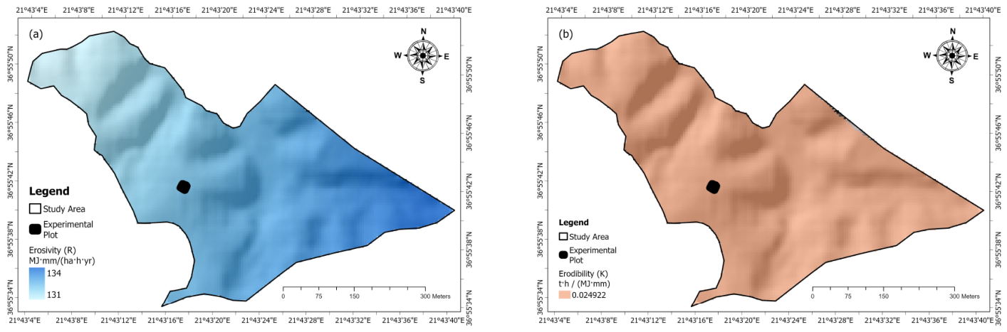
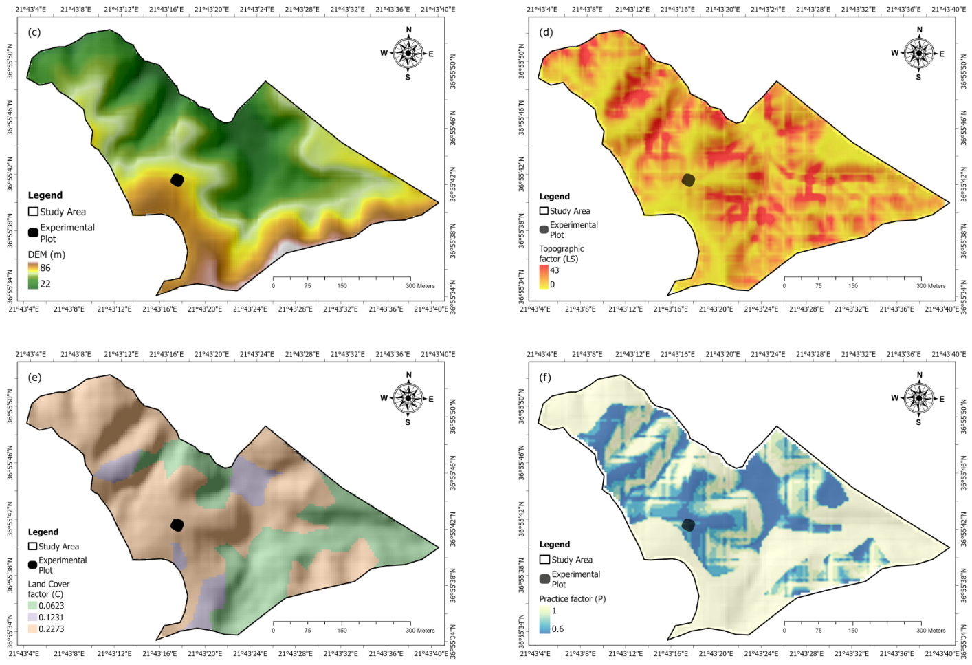
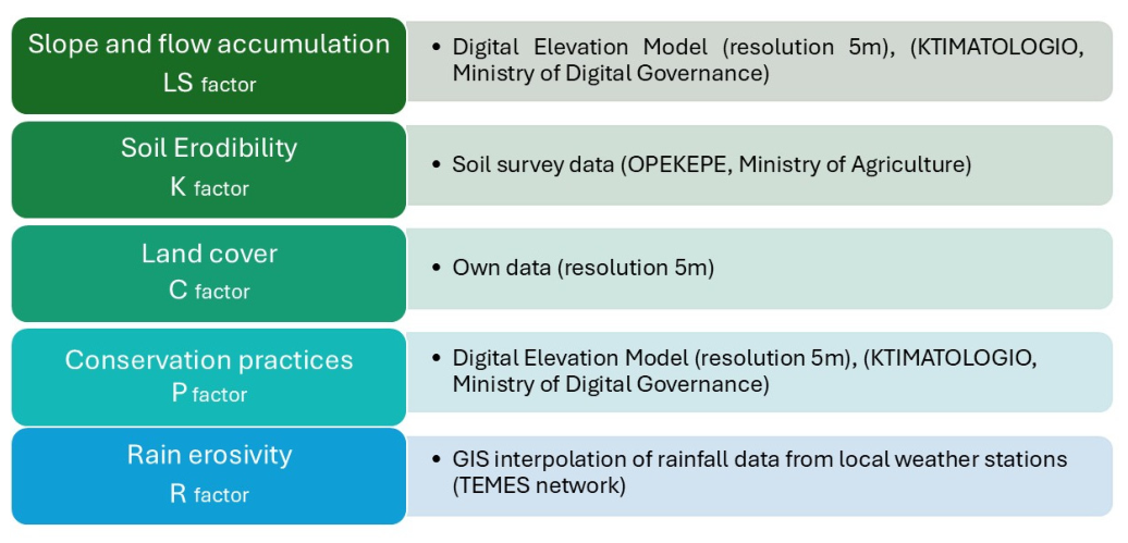
21], and the layers were prepared as gridded rasters at a consistent 5 m spatial resolution, aligned to a common projection and extent. The rasters were then combined using cell-by-cell multiplication to generate a continuous soil loss surface across the study sub-catchment. The GIS workflow followed standard map-algebra practice: (i) preprocess primary inputs (rainfall data, soil properties, DEM, and land cover), (ii) derive R, K, LS, C, and P layers with consistent units and scaling, and (iii) compute A from their product [
35] (
Figure 3).
Because RUSLE predicts long-term average annual soil loss rather than event sediment delivery at the catchment outlet, outputs were interpreted as gross erosion potential (sheet and rill) at the hillslope scale. Measured plot erosion therefore provides a valuable consistency check, but it is not expected to match model output exactly, particularly when monitoring is limited in duration and when local deposition or rill initiation thresholds affect sediment transfer [
22].
2.2.1. Rainfall Erosivity Factor
Rainfall erosivity represents the erosive power of rainfall and its capacity to generate runoff capable of detaching and transporting soil. According to [
33], erosivity is derived from rainfall intensity metrics (e.g., EI30), but such high-frequency records are often unavailable for many Mediterranean monitoring networks. As an alternative, erosivity can be approximated from precipitation totals aggregated at monthly or annual scales [
36].
In this study, R was derived from the modified Fournier framework described by [
37] which documents [
38] Fournier’s original precipitation concentration index to improve correlation with erosivity. For each station, daily rainfall records were aggregated to monthly totals and annual totals. The modified Fournier index (MFI) was computed as:
where P
i is precipitation for month i and P is annual precipitation.
Following the relationship reported by [
39], erosivity was estimated as:
where 0.264 is an empirically derived coefficient obtained from the statistical relationship between MFI and rainfall erosivity (R), ensuring consistency with standard R-factor units.
This precipitation-based erosivity approach is explicitly recommended for application within homogeneous climatic settings, because the F-R relationship can vary across rainfall regimes [
36]. Accordingly, TEMES network (
Figure 4) of 4 rain gauges was selected to represent the same regional climatic domain as the target sub-catchment, and multi-year averaging (2016–2025) was performed to suppress single-year anomalies and better approximate long-term erosive forcing.
Station-level R-factor values were interpolated across the catchment to produce a continuous rainfall erosivity raster at 5 m spatial resolution, consistent with DEM resolution. Interpolation was performed with the IDW (Inverse Distance Weighted) method appropriate to station density and topographic variability, and the resulting raster was clipped to the study-area boundary. The resulting R map was treated as time-invariant for the modelling period, consistent with the long-term average nature of RUSLE.
2.2.2. Soil Erodibility Factor
Soil erodibility (K) describes how easily soil can be detached and carried away by rainfall and runoff under standard reference conditions. It mainly depends on soil texture, organic matter, structure, and how quickly water can move through the soil [
35]. K is usually estimated either from standard-plot measurements or from equations that relate K to measured soil properties (pedotransfer methods).
In this study, the required soil inputs (soil texture, organic matter, soil-structure class, and permeability class) were obtained from the OPEKEPE open soil datasets (Ministry of Rural Development and Food). These spatial layers were used to parameterize the K-factor across the study sub-catchment, ensuring consistent coverage and attribute definitions across land-cover units. To confirm that the mapped properties were representative locally, the OPEKEPE values were validated using field observations and laboratory analyses from soil samples collected at the experimental plot. Agreement was then checked for texture class, organic matter levels, and the assigned structure and permeability classes.
The erodibility factor was computed using the widely cited algebraic approximation of the original USLE nomograph developed by [
33,
35] and reported in metric-converted form (including the 0.1317 unit conversion multiplier [
22]) in authoritative documentation. The equation applied was:
where M is the texture term M = (
msilt +
mvfs) (100 −
mc), with
msilt = percent silt,
mvfs = percent very fine sand, and
mc = percent clay; a is organic matter (%); b is the soil-structure class code (b = 1 for very fine granular, b = 2 for fine granular, b = 3 for medium or coarse granular and b = 4 for blocky, platy or massive); and c is the permeability class code (c = 1 for very rapid and c = 6 for very slow). Six classes are distinguished [
40]: (1) rapid, (2) moderate to rapid, (3) moderate, (4) moderate to slow, (5) slow and (6) very slow. The numerical coefficients in the equation are empirically derived from the original Wischmeier and Smith nomograph [
33] and represent the relative influence of soil texture, organic matter, structure, and permeability on soil erodibility, while 0.1317 is a unit conversion factor to SI units.
A catchment-wide K raster at 5 m resolution was generated by linking computed K values to mapped soil units. The approach ensured that K varied spatially according to dominant soil property patterns while maintaining physical plausibility (e.g., higher K in fine-textured, low-OM soils). This aligns with the conceptual interpretation of K as a soil-property-controlled modifier of erosion susceptibility in RUSLE-type formulations.
2.2.3. Topographic Factor: Slope Length and Steepness
Topography strongly affects erosion because it controls how runoff concentrates and how much energy the flowing water has. In GIS, slope-length effects are often represented using upslope contributing area (the area draining into each cell). This lets the LS factor reflect flow convergence and divergence on complex terrain instead of assuming a uniform hillslope. Accordingly, the combined LS factor was computed using a unit stream power/contributing-area formulation linked to [
41].
where As is the specific catchment area (upslope contributing area per unit contour width), β is the slope angle, m = 0.4 and n = 1.3. The standard slope length of the RUSLE plot is 22.13 m, and 0.0896 corresponds to the sine of the standard 9% slope; both values are used to normalize slope length and steepness in the LS factor calculation.
A hydrologically corrected DEM was used to compute flow direction, flow accumulation, and slope. The contributing-area term As was derived by combining flow accumulation with grid-cell size (i.e., converting accumulated cell counts to contributing area per unit width), while slope was computed in degrees and converted as required for trigonometric functions. This approach captures how runoff concentrates in converging areas of the terrain, which is a key advantage formulation compared with methods that represent slope length only [
42].
2.2.4. Cover-Management Factor
Vegetation and management reduce soil loss by shielding the soil from raindrop impact, increasing hydraulic roughness, and improving infiltration. In RUSLE, this is captured by the cover-management factor C.
Land cover in the study sub-catchment was mapped into a small number of dominant classes that reflect the local landscape (olive groves, sclerophyllous vegetation, and mixed agricultural land with significant natural vegetation). Because the sub-catchment is small and well known, the classification was produced using local knowledge and detailed interpretation. Values for each class (
Table 1) were assigned from published literature values reported by [
43].
2.2.5. Support Practice Factor
The support practice factor (P) reflects the effect of erosion-control practices in reducing soil loss relative to areas without any supporting conservation measure. In this study, the P factor was assigned following the standard procedure of the RUSLE model [
33], based on field verification of existing conservation practices in the study area. Field investigation showed that terracing was the only support practice present in the sub-catchment, while the remaining areas had no identified erosion-control practice due to the prevailing landscape and land-use conditions. Therefore, all non-terraced areas were assigned P = 1.0. For terraced areas, P values were assigned according to slope classes for contour-farmed terraced fields following by [
33]: 0.60 for slopes of 1–2%, 0.50 for 3–8%, 0.60 for 9–12%, 0.70 for 13–16%, 0.80 for 17–20%, 0.90 for 21–25%, and 1.0 for slopes >25%.
2.3. DEMs of Difference Methodology
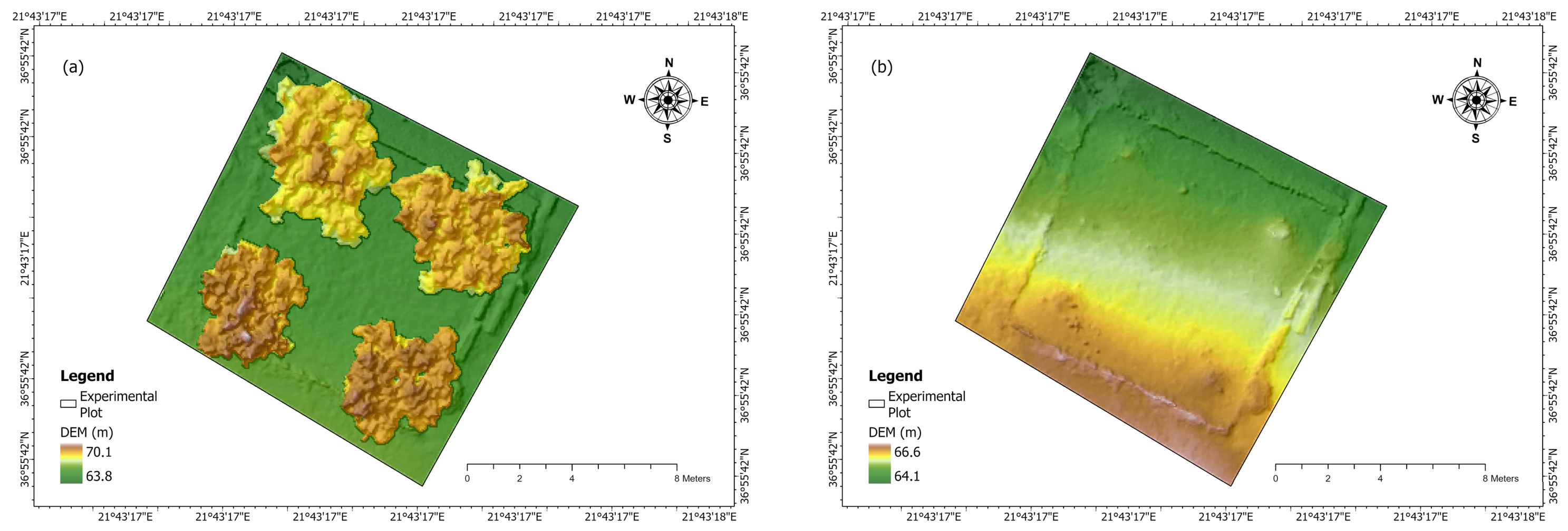
DoD methodology was applied to describe the soil movement within the subplots. The LiDAR sensor has the advantage that vegetation cover can be filtered from the image, allowing detection of soil behavior during a long period with precipitation. Repeat UAV-LiDAR surveys were conducted to derive spatially explicit erosion/deposition estimates. Data acquisition used a DJI Matrice 300 RTK platform carrying a DJI Zenmuse L2 LiDAR payload, manufactured by DJI, Shenzhen, China. The UAV-LiDAR dataset was georeferenced using the RTK-enabled direct positioning capabilities of the Matrice 300 RTK; therefore, no dedicated Ground Control Points (GCPs) were established, as this configuration was considered adequate for the accuracy requirements of the study. The Zenmuse L2 integrates LiDAR with a high-accuracy IMU and supports multi-return acquisition (capturing up to five return signals from each laser pulse). In orchard environments, tree crowns and ground vegetation can partially block the soil surface in image-based reconstructions. Multi-return LiDAR increases the likelihood of obtaining ground observations through canopy gaps [
44]. In contrast, UAV photogrammetry may fail to reconstruct “dead ground” beneath vegetation because it relies on optical visibility [
45].
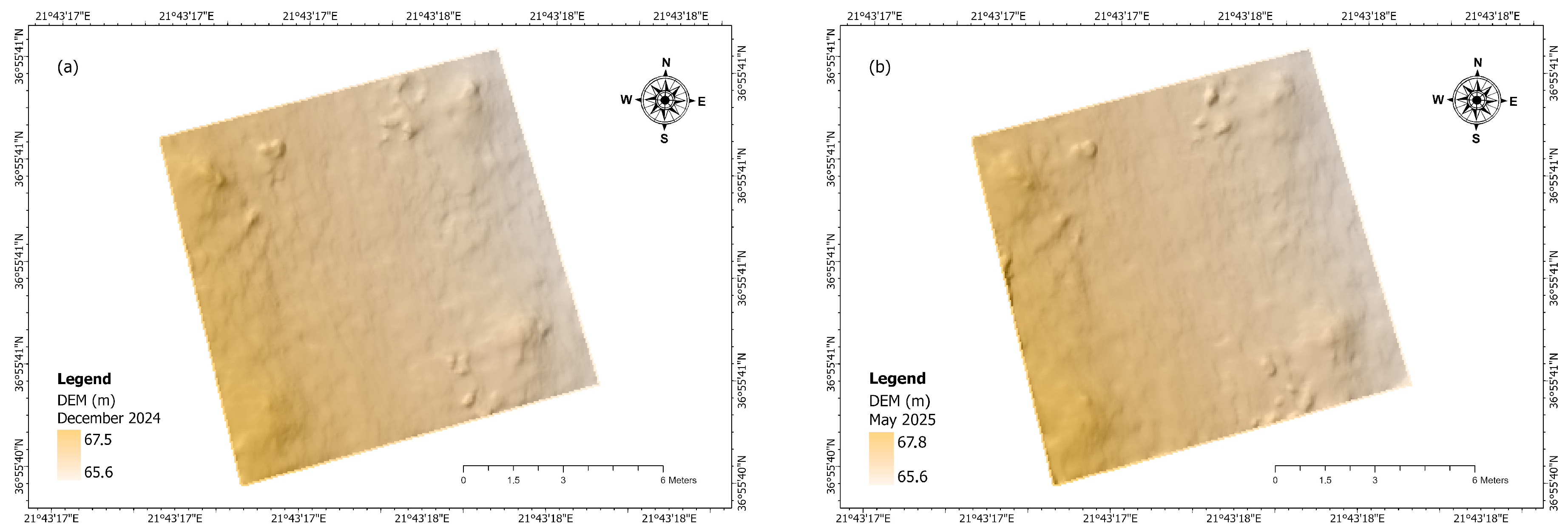
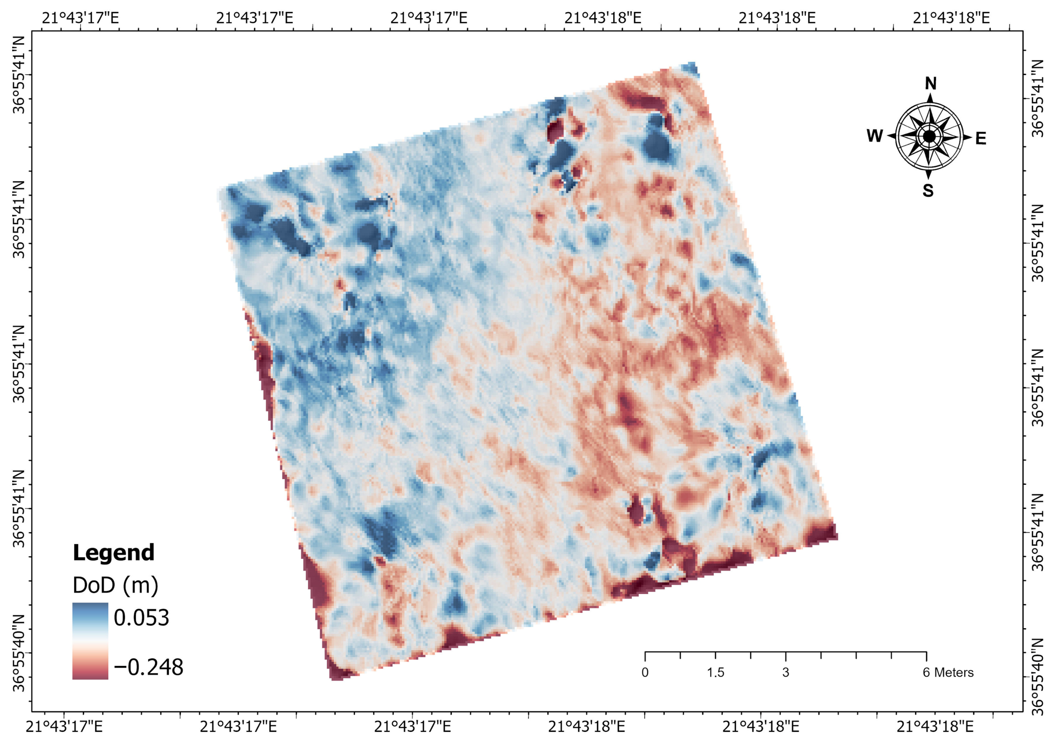
Two flight surveys carried out on 11 December 2024 and 6 May 2025, and each point cloud was processed to generate a gridded DEM at 0.05 m resolution. Point-cloud reconstruction and terrain modelling were performed in DJI Terra. Ground elevations were not derived simply by selecting the “last return.” Instead, a ground-point classification procedure was applied to distinguish bare-earth points from vegetation and other objects. DJI Terra’s dedicated ground-classification workflow was used, with terrain-dependent parameter settings, to generate the DEM from the classified ground points. This distinction matters because ground filtering/classification is a recognized source of uncertainty in terrain modelling under canopy and on complex slopes.
Topographic change between the two dates was quantified using a DEM-of-Difference (DoD):
Following this definition, negative DoD values represent elevation loss (surface lowering/erosion) and positive values represent deposition. The DoD approach is widely used for morphological sediment budgets but requires attention to survey/model uncertainty and the possibility that apparent changes reflect noise rather than geomorphic signal [
46]. DoD values (Δz, m) were converted to per-cell volumes using the grid-cell area:
where A = 0.05 m × 0.05 m = 0.0025 m
2.
Summing ΔVᵢ across all cells yielded the net volumetric change (m
3) over the observation period. Net volume was then converted to mass using the measured average bulk density from the plot (ρb = 1.1 g cm
−3, equivalent to 1.1 t m
−3 by unit conversion), giving
Soil bulk density used to convert net volumetric change to mass was determined from two undisturbed core samples collected at 0–5 cm in the experimental plot using cylinders of 5 cm height [
47]. Bulk density was calculated following [
48] and corrected for the coarse fraction (>2 mm), according to:
where Wc is the oven-dry mass of soil in the cylinder (g), Wg is the mass of gravel (>2 mm) (g), and Vc is the cylinder volume (cm
3).
4. Discussion
The main strength of this study is that soil erosion was examined using a multi-method approach, combining direct field measurements, RUSLE modelling, and LiDAR/DoD-based surface analysis. This is important because soil erosion is a complex process [
49] influenced by multiple factors [
50] acting across different spatial and temporal scales; therefore, a single method is rarely sufficient to capture its full behavior. Recent studies from Mediterranean environments show that runoff plots provide direct field evidence of sediment loss, while GIS- and remote sensing-based models represent the spatial distribution of erosion risk; together, these approaches offer a more complete understanding of erosion processes [
51,
52]. Runoff plots are especially valuable because they provide direct event-scale measurements of gross soil loss [
7,
53], while RUSLE offers spatially distributed predictions of erosion risk [
19,
54,
55], and DoD methods [
56] help visualize how the soil surface changes through time.
Among the methods tested, the runoff-plot experiment provided the most direct measured evidence of soil loss from the monitored subplot [
52,
57]. Runoff plots are widely used to obtain direct measurements of runoff and soil loss from bounded areas, especially at the event scale [
58,
59]. However, their results are sensitive to plot design, operation, and local spatial variability, and should therefore be interpreted with due caution [
58,
60]. In the present study, the runoff-plot data served as the main measured reference for event-driven soil loss. Technical problems in the collection system caused some missing observations during the first monitoring year. Since this period did not coincide with intense rainfall events, major soil-loss events were unlikely to have been missed.
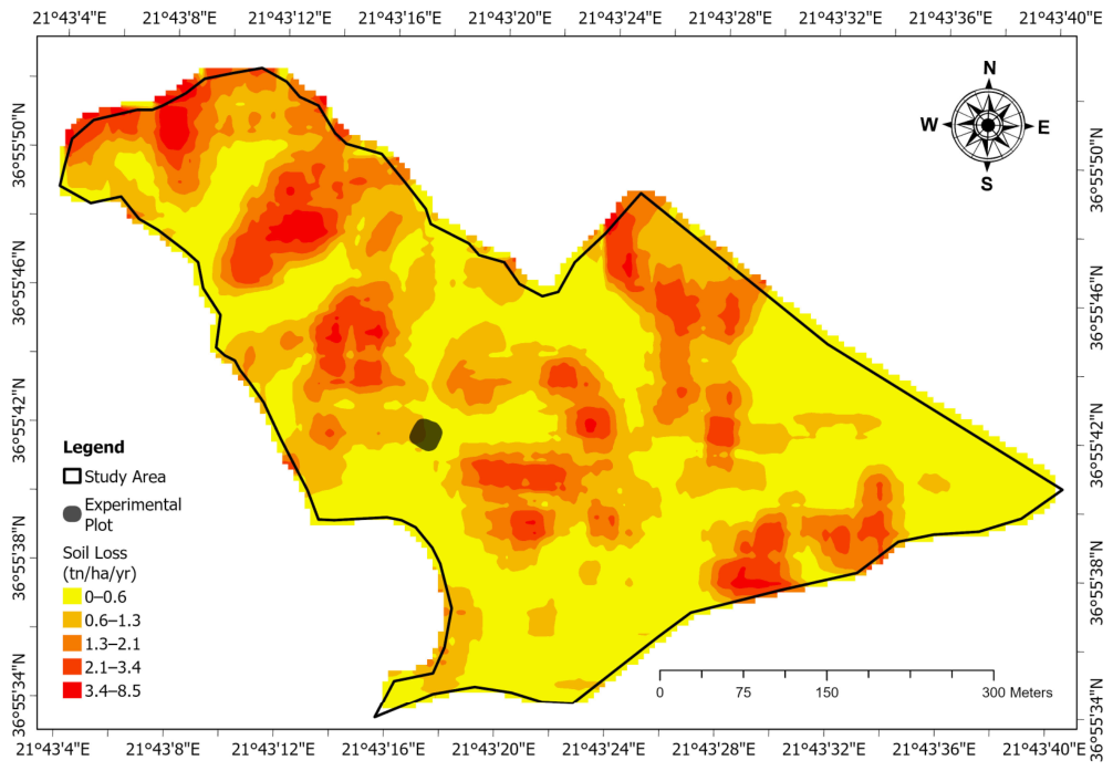
The RUSLE results showed good agreement with the field measurements once the comparison was made at the appropriate spatial scale. This is one of the most important outcomes of this study. The measured annual soil loss values of 0.497 t ha
−1 for 2023–2024 and 0.768 t ha
−1 for 2024–2025 fall within, or very close to, the 0.6–1.3 t ha
−1 yr
−1 range predicted by RUSLE for the pixels corresponding to the experimental plot. This does not mean that the two approaches are identical, but it does indicate that they are in the same order of magnitude and that the model reproduced the local erosion signal reasonably well. This agreement is particularly meaningful because RUSLE is one of the most widely used empirical models for estimating soil erosion [
22], yet its performance depends strongly on the quality of the input layers used to derive the R, K, LS, C, and P factors [
33]. Reliable RUSLE predictions require well-prepared input data and, whenever possible, independent validation against field observation [
24,
35]. In the present study, the quality of the local input data was high, and this likely explains why the model outputs were consistent with the measured plot-scale values.
This also helps justify the decision to apply RUSLE to a small, well-defined sub-catchment rather than to the entire Xerias watershed. RUSLE was originally developed for estimating long-term average annual soil loss [
33] and is generally more defensible when applied at plot to small-catchment scales [
61], especially when local information is available for parameterization and some form of field validation is possible. When the model is transferred to larger areas without validation, uncertainty increases because the input factors become more generalized and because deposition processes are not explicitly represented [
19]. In that respect, our study contributes by showing that a sub-catchment-scale application linked to direct field measurements can produce realistic erosion estimates under Mediterranean olive-growing conditions. The contribution is therefore not only the map itself, but also the demonstration that local validation improves confidence in the mapped results.
The LiDAR and DoD analysis added a different but complementary perspective. Unlike runoff plots, which measure exported sediment, the DoD approach mainly reveals surface elevation change [
44], allowing the identification of zones where the soil surface was lowered or raised between surveys. For this reason, in the present work the DoD results are interpreted primarily in terms of soil displacement and local surface redistribution, rather than as a direct estimate of soil loss. This interpretation is consistent with other DoD-based studies, which show that differenced DEMs are particularly effective for mapping where topographic change occurs and for identifying short-distance redistribution patterns across small plots and hillslopes [
62]. In our plot, the DoD pattern supports the general expectation that material tends to move from relatively higher to relatively lower positions, indicating downslope redistribution of soil within the monitored surface.
At the same time, the DoD part of the study should be interpreted as an exploratory but promising component of the overall methodology. The monitored area was relatively small (100 m
2), and the comparison covered only a five-month period, which limits the degree to which broader or longer-term erosion patterns can be inferred. In addition, the usefulness of DoD products depends strongly on the quality of the DEMs and on their spatial resolution, because high-resolution surfaces are needed to preserve microtopographic features that control flow concentration and local erosion. Previous UAV- and LiDAR-based studies have shown that DEM resolution has a strong influence on slope representation, LS estimation, and the visibility of microtopographic change [
63,
64]. For that reason, the DoD results in this study are best viewed as a detailed indicator of surface behaviour at plot scale, rather than as a stand-alone measure of annual soil loss. Even so, they are valuable because they reveal the internal spatial organization of terrain change in a way that neither runoff plots nor RUSLE can show on their own.
Taken together, the three approaches show that soil erosion assessment benefits from a holistic framework. The field experiment supplies direct measurements, RUSLE provides spatial extrapolation and identifies erosion-prone areas, and LiDAR/DoD reveals fine-scale redistribution of the soil surface. This combination responds to a common limitation in erosion research, namely that many studies rely on only one method and therefore capture only one dimension of the process. Recent Mediterranean reviews explicitly call for this kind of multi-method, multi-scale strategy, because each method provides only a partial but useful view of erosion dynamics [
5,
65]. Our work contributes to this discussion by showing that, even in a relatively small Mediterranean sub-catchment, an integrated design can link direct observations with spatial modelling and high-resolution terrain analysis. Future work can build on this framework by extending monitoring duration, enlarging the number of plots, and further refining terrain-based analysis, with the aim of reducing remaining limitations and strengthening comparisons among methods.
5. Conclusions
This study showed that soil erosion assessment in Mediterranean olive-growing areas can be improved through the combined use of direct field measurements, RUSLE modelling, and LiDAR-based terrain analysis. The field experiment provided direct evidence of actual soil loss at the subplot scale, while the RUSLE model offered a spatially distributed estimate of erosion risk across the study sub-catchment. The agreement between the measured annual soil loss values and the RUSLE-predicted range at the experimental plot suggests that, when supported by high-quality local input data, RUSLE can provide realistic estimates of soil erosion under local conditions.
The LiDAR–DoD approach contributed an additional and complementary perspective by identifying short-term changes in surface elevation and patterns of local soil redistribution within the experimental plot. Although this method was not used here as a direct measure of soil loss, it proved useful for describing soil displacement and surface behavior over time. Taken together, the three approaches showed that soil erosion is a complex process that cannot be fully captured by a single method and that a multi-method framework can support a more complete understanding of erosion dynamics.
Overall, the findings highlight the importance of integrated erosion assessment not only for estimating soil loss, but also for improving our understanding of land degradation processes in vulnerable Mediterranean agroecosystems. Since soil erosion is one of the main drivers of land degradation, especially in sloping cultivated areas, the combined methodology applied in this study may support more targeted soil conservation and sustainable land management strategies. Future research should further refine these approaches, reduce remaining limitations, and expand monitoring in order to strengthen erosion assessment at both plot and sub-catchment scales.