Spatiotemporal Dynamics and Driving Mechanisms of Vegetation Spring Phenology on the Mongolian Plateau: Insights from XGBoost and SHAP

Abstract

Vegetation spring phenology in drylands is sensitive to climatic and anthropogenic pressures, yet the nonlinear responses of the start of the growing season (SOS) across different vegetation types remain inadequately quantified. Here, we extracted the start of the growing season from 2001 to 2020 Moderate-Resolution Imaging Spectroradiometer (MODIS) Normalized Difference Vegetation Index (NDVI) time series for stable vegetation areas on the Mongolian Plateau (MP) and applied Extreme Gradient Boosting (XGBoost) models with Shapley Additive Explanations (SHAP) analysis to six environmental drivers—precipitation, temperature, windspeed, livestock density, population density, and elevation—across forests, shrublands, and grasslands. The SOS displayed pronounced spatial heterogeneity, with earlier onset in northern forests and shrublands and delayed onset in southern arid grasslands. Forests and shrublands exhibited significant advancing trends of 6.8 and 6.4 days per decade, respectively, while grasslands showed no significant trend. Temperature dominated the SOS variability across all vegetation types, yet the relative importance of other drivers varied; windspeed notably influenced forests, whereas precipitation and elevation were critical for grasslands and shrublands. SHAP analysis revealed strong nonlinearities and threshold effects, including a U-shaped temperature response and a 350 mm precipitation threshold in grasslands, beyond which the SOS responses markedly shifted. These results highlight the vegetation-specific and nonlinear nature of phenological regulation in drylands, suggesting that phenology prediction and ecosystem monitoring should explicitly incorporate vegetation type and threshold-based climatic responses.

1. Introduction

Vegetation phenology is a key indicator of ecosystem responses to climate change. Among phenological metrics, the SOS is widely used to reflect vegetation activity and ecosystem productivity [1]. Changes in SOS can directly influence carbon cycling, water balance, and energy exchange. Therefore, understanding the dynamics of SOS is essential for evaluating ecosystem responses under global climate change [2,3].

Arid and semi-arid regions are particularly sensitive to environmental changes due to water limitations and fragile ecosystems [4,5]. The MP is one of the largest dryland regions in the world and is dominated by grassland, shrubland, and forest ecosystems [6]. In recent decades, this region has experienced significant climate variability and increasing human activities, such as grazing and population expansion. These factors may strongly affect vegetation phenology [7,8]. However, compared with humid regions, studies on phenological dynamics in dryland ecosystems remain limited, particularly regarding the differential responses of forest, shrubland, and grassland ecosystems to multiple environmental drivers [9].

Previous studies have explored the relationships between SOS and environmental factors, mainly focusing on climate variables such as temperature and precipitation [10]. However, several limitations still exist. First, many studies are based on statistical relationships that assume simple or monotonic responses, which may fail to capture complex nonlinear behaviors [11]. Second, threshold effects of environmental drivers are often insufficiently quantified, although vegetation responses are rarely linear in dryland ecosystems [12,13]. Third, the influence of human activities, such as livestock density and population pressure, has received relatively less attention [14,15]. In addition, differences among vegetation types, including forest, shrubland, and grassland, are often not explicitly considered, despite their distinct ecological characteristics [16,17].

Based on these gaps, this study aims to address the following questions in the MP: (1) Has SOS exhibited significant temporal changes and spatial heterogeneity from 2001 to 2020? (2) What are the dominant driving factors controlling SOS dynamics, and what is the relative contribution of climatic versus anthropogenic variables? (3) Do nonlinear relationships and threshold effects exist between SOS and its driving factors, and do these relationships vary across vegetation types?

To answer these questions, this study first extracts SOS from the long-term NDVI time series within stable vegetation areas to minimize the influence of land-use change. Then, multiple driving factors, including climate variables, topographic conditions, and human activities, are integrated into an XGBoost model. The SHAP method is further applied to quantify the relative importance of each factor and to reveal their nonlinear effects and thresholds. This framework enables a comprehensive understanding of vegetation phenology dynamics and their associated influencing factors in dryland ecosystems.

2. Materials and Methods

2.1. Study Area

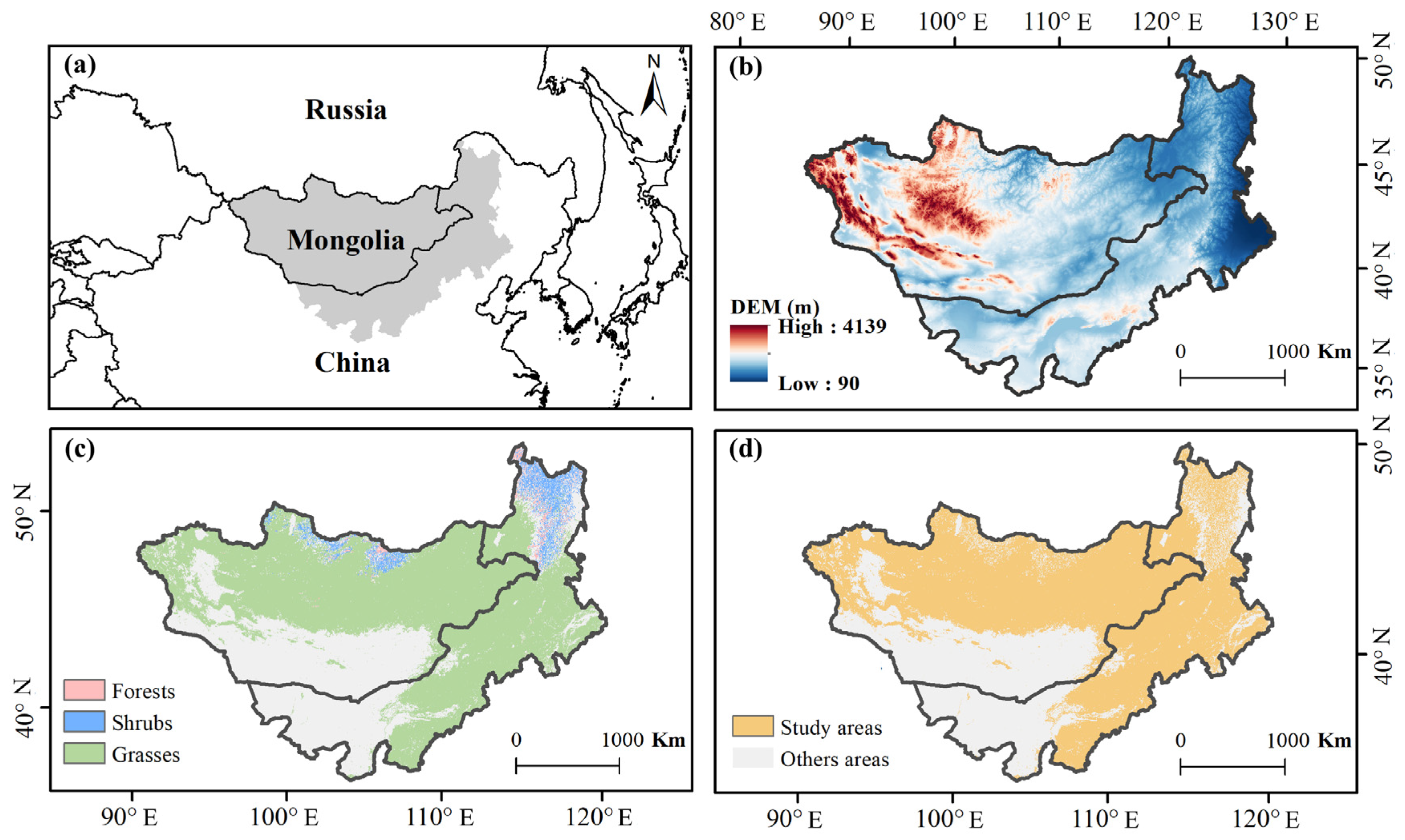
The study area is located in the MP (37°22′–53°20′ N and 87°43′–126°04′ E), encompassing parts of Mongolia and Inner Mongolia, China (Figure 1a). The region has a continental climate, with cold and dry winters and warm, moderately wet summers. Mean annual temperature ranges from −5 °C to 8 °C, and mean annual precipitation decreases from approximately 400 mm in the north to less than 100 mm in the south, following a northeast–southwest gradient. Elevation varies from about 500 m to over 3000 m (Figure 1b). The Altai, Khangai, and Khentii mountains dominate the western and northern parts, while the eastern and southern regions are characterized by low-lying plains and plateaus.

The natural vegetation consists primarily of forest, shrubland, and grassland (Figure 1c). Forest is mainly distributed in the northern mountain ranges, dominated by larch (Larix sibirica Ledeb) and birch (Betula pendula subsp. mandshurica (Regel) Ashburner & McAll). Shrubland occurs in transitional zones between forest and grassland [18]. Grassland, including meadow steppe, typical steppe, and desert steppe, occupies the largest proportion of the study area [19]. To eliminate the influence of non-vegetated areas on phenological detection, this analysis included only those areas where the land cover type remained stable and the NDVI exceeded 0.1 throughout the study period (Figure 1d).

2.2. Datasets and Processing

To facilitate subsequent research, all datasets were processed uniformly using ArcGIS 10.2 and resampled to a spatial resolution of 1000 m.

2.2.1. Vegetation Cover Type Data

We obtained land use type data for the years 2001 and 2020 from the Moderate-Resolution Imaging Spectroradiometer (MODIS) MCD12Q1 V6 (https://modis.gsfc.nasa.gov/, accessed on 25 March 2026). This data was used to identify stable vegetation areas. Specifically, pixels that were classified as vegetation in both 2001 and 2020 are considered stable. Pixels with any land cover conversion between the two time points were excluded. These stable areas were subsequently designated as the study areas for this research. The dataset defines 17 major land cover types. In this study, classes 1 through 5 were reclassified as forests, classes 6 through 9 as shrublands, and class 10 as grasslands. Additionally, classes 11 through 17—representing non-vegetated cover—were excluded to ensure they would not interfere with the monitoring of vegetation phenology (

Table 1. The reclassification of land use type.

Original Serial Number	Original Land Use Type	Serial Number After Reclassification	Land Use Type After Reclassification
1	Evergreen Needleleaf Forests	1	Forests
2	Evergreen Broadleaf Forests
3	Deciduous Needleleaf Forests
4	Deciduous Broadleaf Forests
5	Mixed Forests
6	Closed Shrublands	2	Shrubs
7	Open Shrublands
8	Woody Savannas
9	Savannas
10	Grasslands	3	Grasses
11	Permanent Wetlands	0	Other Areas
12	Cropland
13	Urban and Built-up Lands
14	Cropland/Natural Vegetation Mosaics
15	Permanent Snow and Ice
16	Non-Vegetated Lands
17	Water Bodies

).

2.2.2. Vegetation Phenology Data

Vegetation phenology was derived from the MODIS MOD13Q1 Collection 6 product, which provides 16-day composite NDVI at a spatial resolution of 250 m (https://modis.gsfc.nasa.gov/, accessed on 25 March 2026). The study period covered 2001 to 2020. All available images within the study area were filtered and preprocessed. Pixels with NDVI below 0.1 were excluded to minimize noise from non-vegetated surfaces.

The SOS was extracted using a threshold-based method [20]. For each pixel and each year, the minimum and maximum NDVI were calculated. A dynamic threshold was defined as the minimum NDVI plus a fixed percentage (20%) of the annual NDVI amplitude [21]. The SOS was then identified as the first day of the year (DOY) on which NDVI exceeded this threshold [22]. To ensure data quality, only pixels with stable land cover during the study period were retained, based on a pre-defined stable mask.

2.2.3. Data on Driving Factors

Six driving factors were selected for this study (

Table 2. Driving factors’ data sources.

Data Name	Time Range	Native Resolution	Source
Precipitation (PRE) (mm)	2001–2020	11 km	ERA5-LAND (GEE) (https://earthengine.google.com/)
Temperature (TEM) (°C)	2001–2020	11 km
Windspeed (WIN) (m/s)	2001–2020	10 km
Population Density (POP)	2001–2020	1 km	Worldpop (https://www.worldpop.org/)
Livestock Density (DENSITY) (Head/km2)	2001–2020	1 km	https://figshare.com/articles/dataset/gridded_livestock_mongolian_plateau_2000_2020/28695728?file=56397962 (accessed on 25 March 2026)
digital elevation model (DEM) (m)	2001	500 m	SRTM (GEE) (https://earthengine.google.com/)

). These included three climate variables (precipitation, temperature, and windspeed), two human activity variables (population density and livestock density), and one topographic variable (digital elevation model). All driving factor datasets were resampled to a consistent spatial resolution and projected to the same coordinate system before analysis.

2.3. Methods

2.3.1. SOS Extraction

The SOS was derived from the MODIS NDVI time series (MOD13Q1) from 2001 to 2020. We used a threshold-based method combined with smoothing techniques to reduce noise.

First, we applied the Savitzky–Golay filter to smooth the original NDVI time series. This filter reduces noise caused by cloud contamination and atmospheric variability while preserving seasonal patterns [23]. We extracted SOS for each pixel and each year using a dynamic threshold [21]. For a given year, let ${NDVI}_{min}$ and ${NDVI}_{max}$ be the minimum and maximum NDVI values. The annual NDVI amplitude was calculated as:

$$A= {NDVI}_{max}-{NDVI}_{min}$$

(1)

The threshold (${NDVI}_{th}$) was then defined as:

$${NDVI}_{th}={NDVI}_{min}+\alpha \times A$$

(2)

where $\alpha$ is the threshold ratio. In this study, $\alpha$ was set to 0.2 following previous phenological studies.

The SOS was identified as the first DOY on which the smoothed NDVI exceeded ${NDVI}_{th}$ and remained above it for at least three consecutive observations. This rule avoids false detections caused by short-term noise [22,24]. Only pixels with NDVI > 0.1 throughout the year were retained to exclude non-vegetated areas.

2.3.2. Trend Analysis

The temporal trends of the start of the SOS from 2001 to 2020 were analyzed on a per-pixel basis using the non-parametric Theil–Sen slope estimator in conjunction with the Mann–Kendall (MK) significance test [25,26,27]. This combined approach is widely employed in vegetation phenology studies because it is robust against outliers and does not require assumptions of data normality [28].

The Sen’s slope ($\beta$) quantifies the magnitude of the monotonic trend in a time series. For a given pixel, let $x_1, x_2,\dots , x_n$ denote the annual SOS values over $n$ years. The slope between any pair of years $i$ and $j(1\le i<j\le n)$ is calculated as:

$${\beta }_{ij}={\displaystyle \frac{x_j-x_i}{j-i}}$$

(3)

The overall Sen’s slope estimator is defined as the median of all $N=n(n-1)/2$ pairwise slopes:

$$\beta =median\left\{{\beta }_{ij}\left|1\le i<j\le n\right.\right\}$$

(4)

A positive $\beta$ indicates a delaying trend in SOS (later green-up), whereas a negative $\beta$ signifies an advancing trend (earlier green-up). The magnitude of $\beta$ represents the average annual rate of change in days per year.

The MK test evaluates the statistical significance of the detected trend. The test statistic $S$ is computed as:

$$S={\displaystyle \sum _{i=1}^{n-1}}{\displaystyle \sum _{j=i+1}^n}sgn\left(x_j-x_i\right)$$

(5)

where the sign function $sgn\left(\theta \right)$ is defined as:

$$sgn\left(\theta \right)=\left\{\begin{array}{c}+1,if \theta >0\\ 0, if \theta =0\\ -1,if \theta <0\end{array}\right.$$

(6)

For $n\ge 10$, the statistic $S$ is approximately normally distributed with mean $E\left(S\right)=0$ and variance:

$$Var\left(S\right)={\displaystyle \frac{n\left(n-1\right)\left(2n+5\right)}{18}}$$

(7)

The standardized test statistic $Z$ is then calculated as:

$$Z=\left\{\begin{array}{c}{\displaystyle \frac{S-1}{\sqrt{Var\left(S\right)}}},if S>0\\ 0, if S=0\\ {\displaystyle \frac{S+1}{\sqrt{Var\left(S\right)}}},if S<0\end{array}\right.$$

(8)

A positive $Z$ value indicates an upward trend, while a negative $Z$ value indicates a downward trend. The absolute value $\mid Z\mid$ is compared against critical values from the standard normal distribution to assess significance.

Following previously established significance thresholds, the SOS trends were classified into seven categories by integrating the direction of the Sen’s slope ($\beta$) with the absolute $Z$ value from the MK test [16]. The detailed classification criteria are summarized in

Table 3. Classification criteria for SOS trends based on Sen’s slope (β) and MK Z-values.

Trend Direction	$\left|\mathit{Z}\right|$ Range	Category	Abbreviation	Significance Level
$\beta > 0$ (Delaying SOS)	$\left|Z\right| \ge 2.58$	Extremely significant increase	ES+	p < 0.01
	$1.96 \le \left|Z\right|<2.58$	Significant increase	S+	p < 0.05
	$1.645 \le \left|Z\right|<1.96$	Slightly significant increase	SS+	p < 0.10
$\beta < 0$ (Advancing SOS)	$\left|Z\right| \ge 2.58$	Extremely significant decrease	ES−	p < 0.01
	$1.96 \le \left|Z\right|<2.58$	Significant decrease	S−	p < 0.05
	$1.645 \le \left|Z\right|<1.96$	Slightly significant decrease	SS−	p < 0.10
$\beta \approx 0$ or any sign	$\left|Z\right|<1.645$	No trend	NT	p ≥ 0.10

Note: The critical Z-values 1.645, 1.96, and 2.58 correspond to the 90%, 95%, and 99% confidence levels (two-tailed test), respectively.

.

2.3.3. Multicollinearity Test

Before constructing the XGBoost model, we conducted a multicollinearity test to avoid redundant information among explanatory variables. The variance inflation factor (VIF) was used to quantify the degree of linear correlation between variables. A higher VIF indicates stronger multicollinearity, while the reciprocal (1/VIF) represents the proportion of unique information contributed by each variable [29].

Following common thresholds, variables with VIF greater than 10 were considered to have severe multicollinearity and were excluded. In this study, all variables had VIF values well below 10, indicating acceptable levels of multicollinearity.

We performed separate VIF analyses for forest, shrubland, and grassland ecosystems due to their different environmental conditions. The results are shown in

Table 4. Multicollinearity diagnostics for each vegetation type.

Variable	Forests		Shrubs		Grasses
	VIF	1/VIF	VIF	1/VIF	VIF	1/VIF
WIN	1.37	0.732	1.11	0.904	1.07	0.935
TEM	1.41	0.708	1.82	0.550	5.54	0.180
DENSITY	1.34	0.748	1.22	0.820	1.03	0.969
DEM	1.26	0.793	1.71	0.585	4.63	0.216
PRE	1.28	0.782	1.10	0.911	1.53	0.654
POP	1.01	0.993	1.00	0.996	1.02	0.983
Mean VIF	1.28		1.33		2.47

.

For all three vegetation types, the mean VIF values were below 3, and all individual VIF values were less than 6. This indicates that multicollinearity among the selected driving factors was low. Therefore, all six variables were retained for subsequent XGBoost modeling and SHAP analysis.

2.3.4. XGBoost Model

The nonlinear responses of SOS to multiple environmental drivers were examined using the XGBoost algorithm. XGBoost is an ensemble learning method that constructs a series of decision trees in a sequential manner, where each new tree corrects the errors made by the previous ones [30]. Owing to its capacity to accommodate complex interactions and heterogeneous input data, this technique is increasingly adopted in ecological applications [31].

Based on the VIF diagnostics, all six candidate predictors were retained for model construction. These predictors encompassed three climatic variables—PRE, TEM, and WIN—along with two anthropogenic indicators—DENSITY and POP—and one topographic descriptor, DEM. The SOS served as the response variable. Separate XGBoost models were developed for forest, shrubland, and grassland ecosystems to account for their distinct ecological characteristics.

The XGBoost algorithm minimizes a regularized objective function that integrates a loss term and a penalty component:

$$Obj={\displaystyle \sum _{i=1}^n}L\left(y_i,{\widehat{y}}_i\right)+{\displaystyle \sum _{k=1}^K}\mathsf{\Omega }\left(f_k\right)$$

(9)

where $L\left(y_i,{\widehat{y}}_i\right)$ measures the difference between the observed SOS ($y_i$) and the predicted value (${\widehat{y}}_i$). The term $\mathsf{\Omega }\left(f_k\right)$ is a regularization function that penalizes the number of trees and the depth of each tree. This regularization reduces overfitting and improves model generalization. In contrast to conventional linear regression, XGBoost imposes no assumptions of linearity or normality on the data, rendering it particularly suitable for detecting nonlinearities and threshold behaviors in the relationship between phenological metrics and environmental forcing. For each vegetation type, the modeling dataset consisted of all valid pixel–year samples within the corresponding vegetation class, resulting in sufficiently large sample sizes for model training. The dataset was randomly divided into a training subset (70%) and a validation subset (30%) using a fixed random seed (123) to ensure reproducibility. The XGBoost model was implemented using a gradient boosting framework with the squared error loss function. Key hyperparameters were set to balance model complexity and generalization ability, including a maximum tree depth of 8, a learning rate of 0.09. To allow flexible tree construction, the minimum child weight was set to 10, and regularization terms were minimized.

In addition to the coefficient of determination (R²), model performance was further evaluated using root mean square error (RMSE) and mean absolute error (MAE), providing a more comprehensive assessment of predictive accuracy.

2.3.5. SHAP Analysis

To elucidate the contributions of individual predictors, we applied SHAP, a method grounded in cooperative game theory. In the SHAP framework, the prediction generated by the model is regarded as a collective payout, and each explanatory variable is treated as a player whose marginal contribution to the prediction is evaluated across all conceivable combinations of features [32].

For a given variable $i$, its Shapley value ${\varphi }_i$ is calculated as a weighted average of its marginal contributions across all possible variable subsets:

$${\varphi }_i=\sum _{S\subseteq N\backslash \left\{i\right\}}{\displaystyle \frac{\left|S\right|!\left(\left|N\right|-\left|S\right|-1\right)!}{\left|N\right|!}}\left[v\left(S\cup \left\{i\right\}\right)-v\left(S\right)\right]$$

(10)

where $N$ is the full set of explanatory variables, $S$ is any subset that does not include feature $i$, and $v\left(S\right)$ is the model prediction based on subset $S$. A positive SHAP value means the variable pushes the SOS prediction toward a later date. A negative value means it pushes SOS toward an earlier date.

Both global and local interpretability were pursued. Globally, variable importance was assessed by averaging the absolute SHAP values across all observations—larger mean absolute SHAP values signifying greater overall influence on SOS prediction. Locally, SHAP dependence plots were constructed to visualize how the predicted SOS varies along the gradient of an individual driver while accounting for the average effects of all other covariates. SHAP dependence curves were constructed by plotting feature values against their corresponding SHAP values and applying locally weighted regression (LOESS) smoothing to capture the underlying nonlinear trends. Thresholds were identified as the points where the smoothed SHAP curves cross zero or exhibit clear inflection behavior, indicating transitions between delaying and advancing effects on SOS.

Through the combined XGBoost–SHAP analytical framework, we achieved both high predictive accuracy and transparent model interpretation. This approach enabled the quantification of predictor importance and the characterization of nonlinear, ecosystem-specific responses of spring phenology to climatic and anthropogenic drivers.

3. Results

3.1. Spatial Pattern of SOS

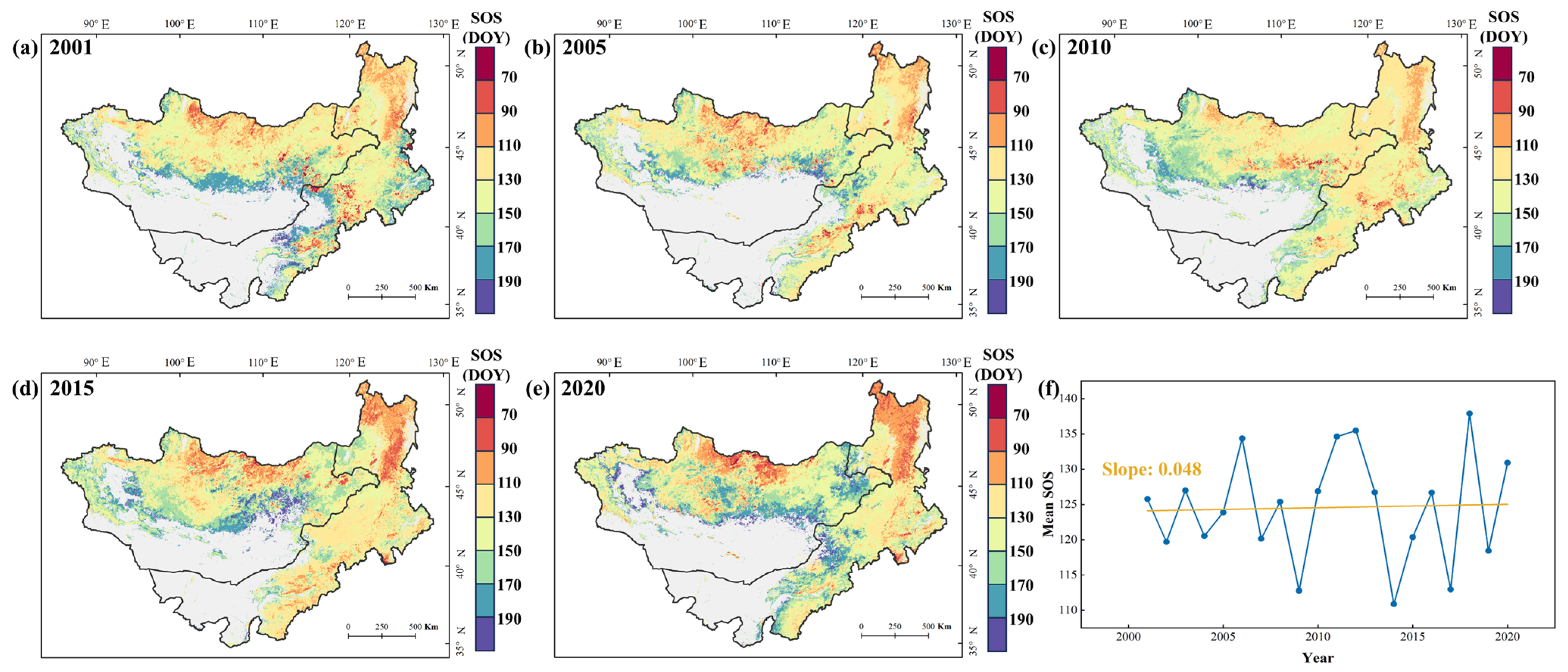
The spatial distribution of SOS across the MP from 2001 to 2020 is shown in Figure 2. Clear spatial heterogeneity is observed. In general, SOS occurs later in the southwestern region and earlier in the northern and eastern parts of the study area.

This pattern is closely related to vegetation distribution. The northeastern region is mainly dominated by forest and shrubland, where SOS tends to occur earlier. In contrast, the southwestern region is largely covered by grassland, where SOS is relatively delayed, possibly due to stronger water limitation and slower vegetation response to early-season temperature increases. In addition, grasslands located in the southeastern region show relatively earlier SOS compared to other grassland areas, which may be associated with anthropogenic influences such as grazing or land-use intensity.

Over the entire study period, the mean SOS was approximately 125 DOY, and no significant overall temporal trend was observed at the regional scale. However, spatial differences in trends are evident. In particular, grassland-dominated areas in the southern region show a tendency toward delayed SOS from 2001 to 2020.

3.2. Temporal Trends of SOS

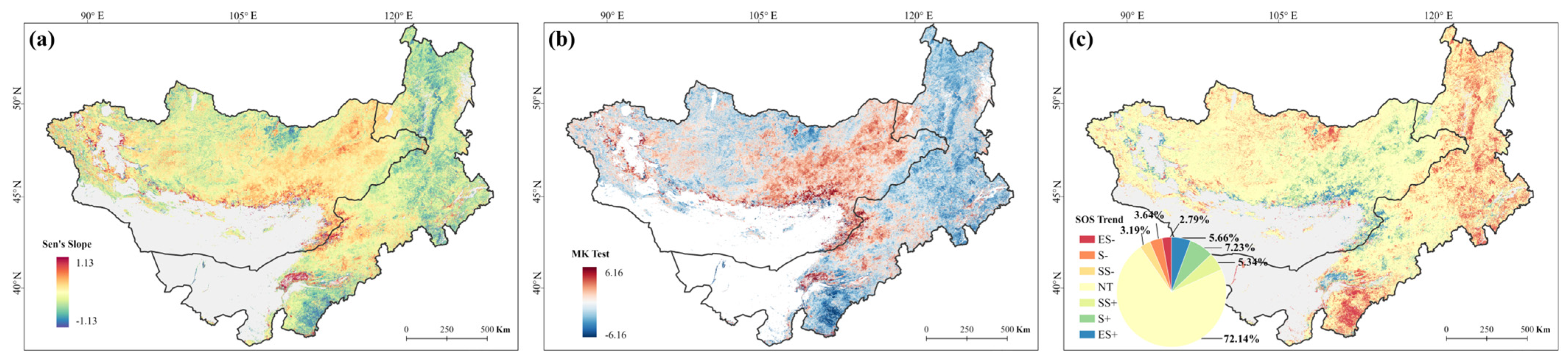
The spatial patterns of the Sen’s slope, MK Z-values, and the derived trend classification for the SOS from 2001 to 2020 are presented in Figure 3. The Sen’s slope estimator ($\beta$) quantifies the magnitude of the phenological shift, whereas the MK test assesses the statistical significance of the detected trends.

The Sen’s slope map (Figure 3a) reveals pronounced spatial heterogeneity in SOS changes across the MP. Negative β values, indicating an advancing SOS, dominate the northern and northeastern portions of the study area, particularly within the forested and mountainous regions of the Khentii and Khangai ranges. In these zones, SOS advancement rates locally exceed −0.8 days per year. Positive β values, reflecting a delayed SOS, are concentrated in the southern and southwestern arid grasslands, with the most substantial delays exceeding 0.8 days per year observed along the desert–steppe transition zone. The magnitude of change decreases toward the central plateau, where β values fluctuate near zero.

The spatial distribution of MK Z-values (Figure 3b) further delineates the statistical robustness of these trends. Extensive areas in the northern forest–steppe ecotone exhibit $\left|Z\right|$ values above 2.58, underscoring the high confidence in the observed SOS advancement. In contrast, large expanses of the central and southern grasslands display $\left|Z\right|$ values below 1.645, indicating that the detected delays or minor fluctuations in these water-limited regions are not statistically distinguishable from interannual variability.

The integrated trend classification (Figure 3c) synthesizes the direction and significance of SOS change. ES− and S− categories are predominantly clustered in the northern montane forests and adjacent shrublands, where warming has likely exerted a dominant and consistent forcing on spring phenology. Conversely, ES+ and S+ categories are sparsely distributed and primarily confined to the southwestern desert steppe, suggesting that localized drought stress or other environmental constraints have systematically postponed green-up onset. The majority of areas exhibiting no significant trend in SOS are distributed across grassland ecosystems. After excluding these non-significant regions, approximately 34.56% of the remaining area (i.e., areas with significant trends) shows a delayed spring phenology. Within this delayed subset, 28.99%, 37.85%, and 33.16% correspond to extremely significant delay, significant delay, and slightly significant delay, respectively, with these categories predominantly clustered in the southern grassland zone. In contrast, the remaining 65.44% of the significantly changing area exhibits an advancing SOS trend. Within this advancing subset, 31.03%, 39.68%, and 29.29% correspond to extremely significant advance, significant advance, and slightly significant advance, respectively. This pattern highlights the contrasting phenological sensitivities of different vegetation types, with forests showing a stronger advancing tendency, while grasslands exhibit weaker and largely non-significant responses.

3.3. Differences Among Vegetation Types

Although the overall SOS trend in the study area is not significant, clear differences emerge when analyzing vegetation types separately. The timing and trends of spring phenology vary substantially among forest, shrubland, and grassland (Figure 4).

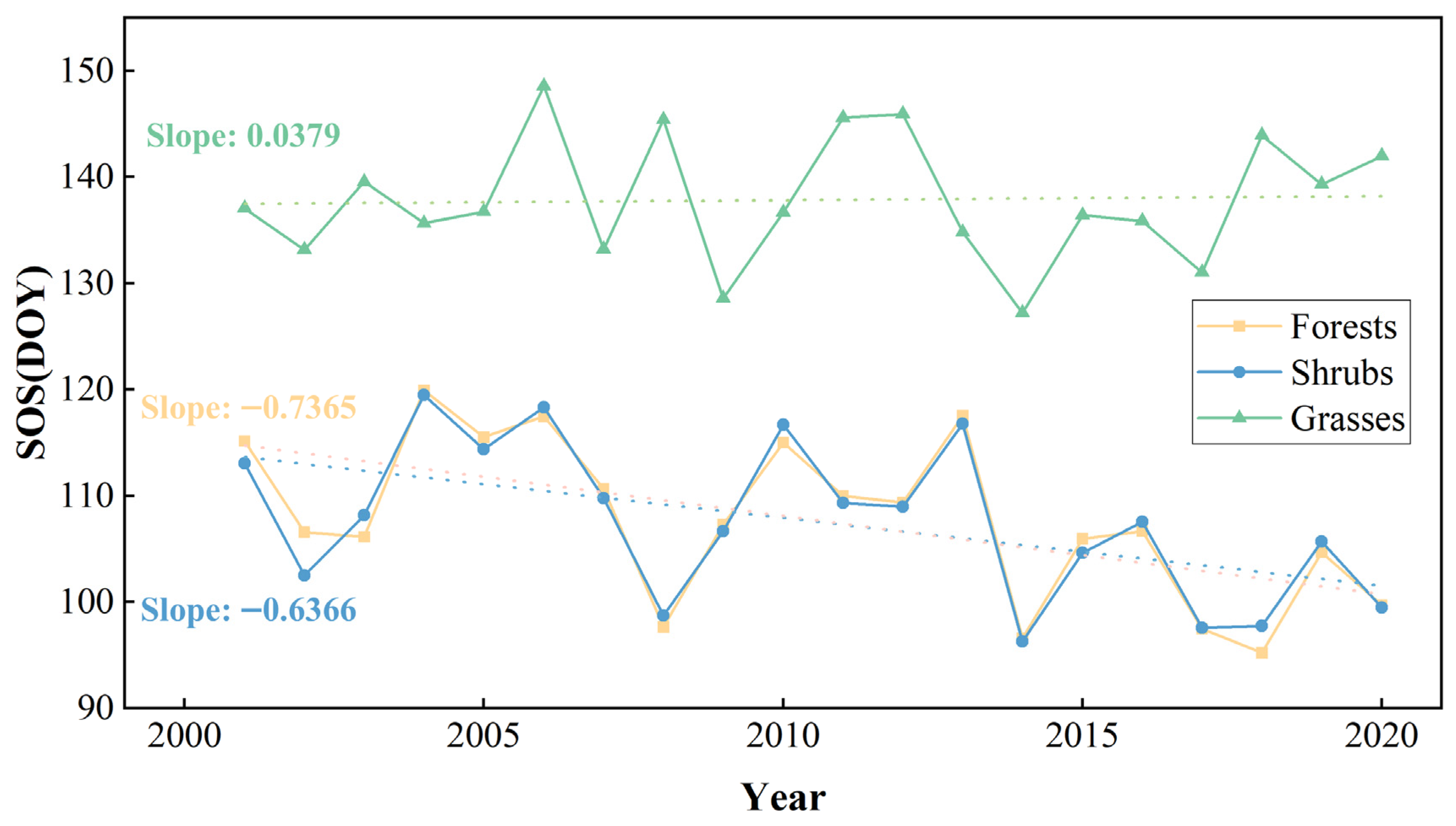
Forests exhibit the earliest SOS, with an average value of 107.72 DOY, and show a significant advancing trend of approximately 6.82 days per decade (n = 20, t = −2.98, p < 0.05). Shrubland shows a similar pattern, with a mean SOS of 107.59 DOY and a significant advancement of about 6.36 days per decade (n = 20, t = −2.55, p < 0.05). The trends in forest and shrubland are highly consistent. In contrast, grassland has the latest SOS, with an average of 137.82 DOY, and shows no significant trend over time, with a slight delay of about 0.75 days per decade (n = 20, t = 0.16, p = 0.787).

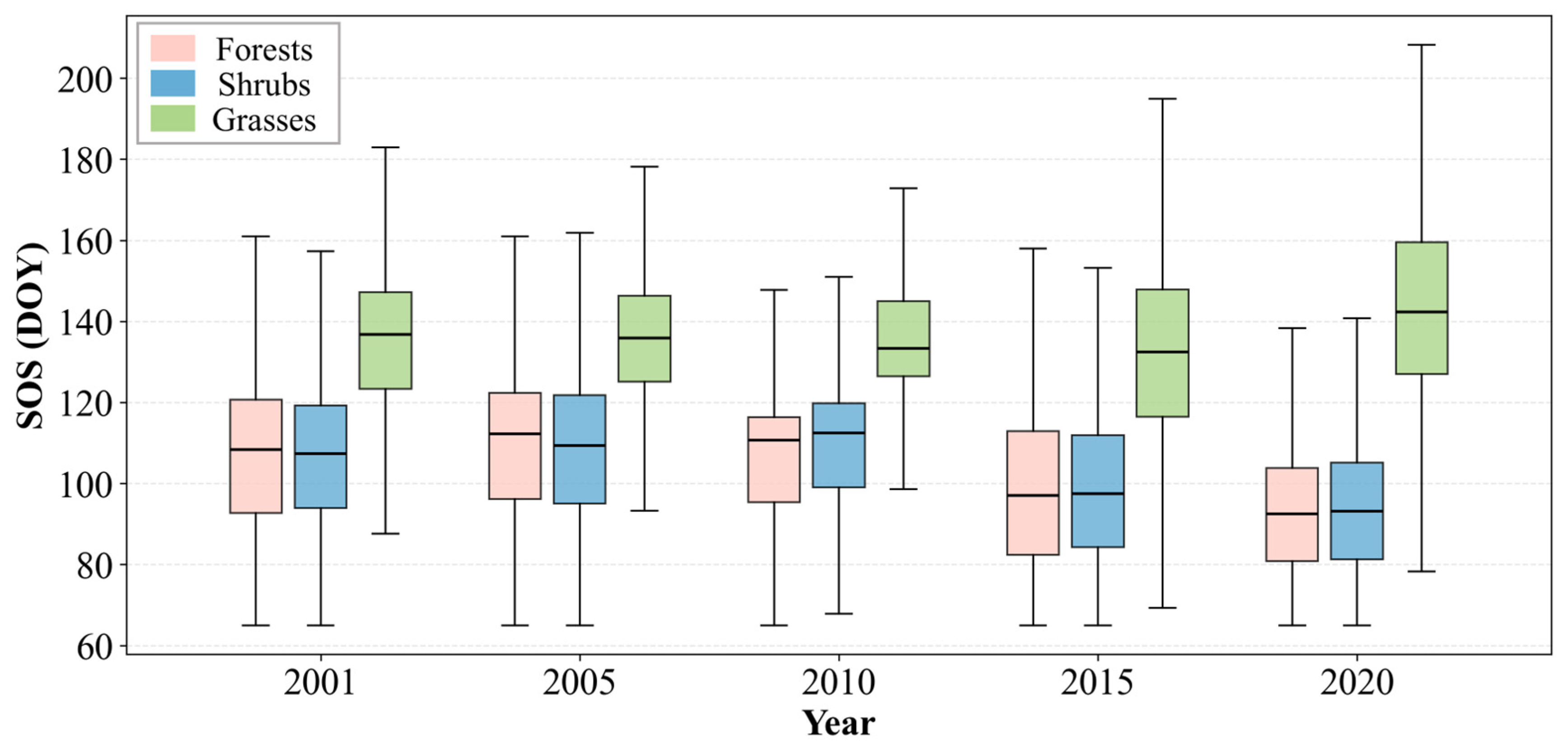
To further examine interannual variations, the temporal dynamics of SOS for each vegetation type were analyzed (Figure 5). From 2001 to 2020, grassland consistently exhibits later SOS than forest and shrubland. Forest and shrubland show similar temporal patterns, with a clear advancing trend. The mean SOS for both vegetation types decreases from approximately 106 DOY in 2001 to around 94–95 DOY in 2020. In contrast, grassland displays a different pattern. From 2001 to 2015, SOS remains relatively stable, ranging between 133 and 136 DOY. However, a noticeable delay occurs in 2020, with the mean SOS increasing to approximately 143 DOY. This divergence suggests that grassland phenology may be more sensitive to short-term environmental fluctuations or external disturbances compared to forest and shrubland ecosystems.

3.4. Driving Factors of SOS

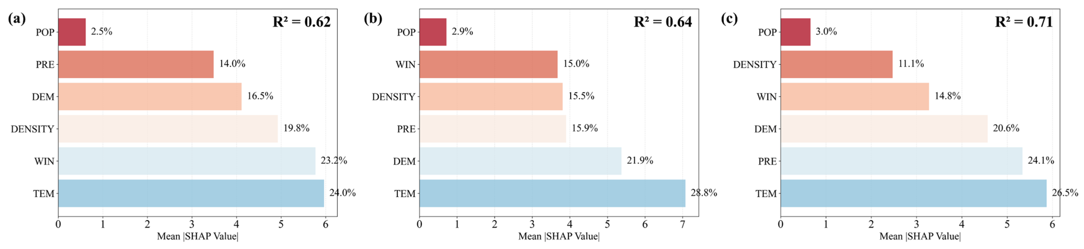
The performance of the XGBoost model for different vegetation types is shown by the R². The model demonstrates good predictive ability for SOS across all vegetation types. For forests, shrubs and grasses, with the R² ranging from a minimum of 0.62 to a maximum of 0.71. These results indicate that the model can effectively capture the relationships between SOS and environmental drivers, with relatively better generalization performance in grassland ecosystems.

The relative importance of driving factors varies among vegetation types (Figure 6). Overall, TEM emerges as a dominant driver across all vegetation types, indicating that thermal conditions play a fundamental role in controlling SOS in the MP. In addition, climate-related factors generally contribute more than human-related variables.

For forests (Figure 6a), POP shows the lowest contribution (2.5%), while TEM, WIN, and DENSITY play more important roles, contributing 24.0%, 23.2%, and 19.8%, respectively. This suggests that forest phenology is primarily regulated by climatic conditions, while also being influenced by grazing-related disturbances to a certain extent.

For shrubland (Figure 6b), the contributions of TEM (28.8%), DEM (21.9%), and PRE (15.9%) are relatively prominent, indicating that both thermal conditions and topographic factors play key roles in shaping SOS. POP remains a minor contributor (2.9%). Compared with forests, shrubland SOS appears to be influenced by both climatic and surface environmental conditions. Compared with forests, shrubland SOS appears to be influenced by a combination of climatic and underlying surface conditions, reflecting its transitional ecological characteristics.

For grassland (Figure 6c), TEM (26.5%) is identified as the most important factor, followed by PRE (24.1%) and DEM (20.6%), while POP contributes the least (3.0%). The stronger influence of TEM and PRE suggests that grassland phenology is more directly controlled by hydrothermal conditions, reflecting the high sensitivity of grassland ecosystems to water and heat availability.

Overall, these results highlight both commonalities and differences in the factors associated with SOS among vegetation types. While temperature plays a dominant role across all ecosystems, the relative importance of other factors varies, indicating that vegetation-specific responses should be considered when analyzing phenological dynamics in dryland regions.

3.5. Nonlinear Effects and Thresholds

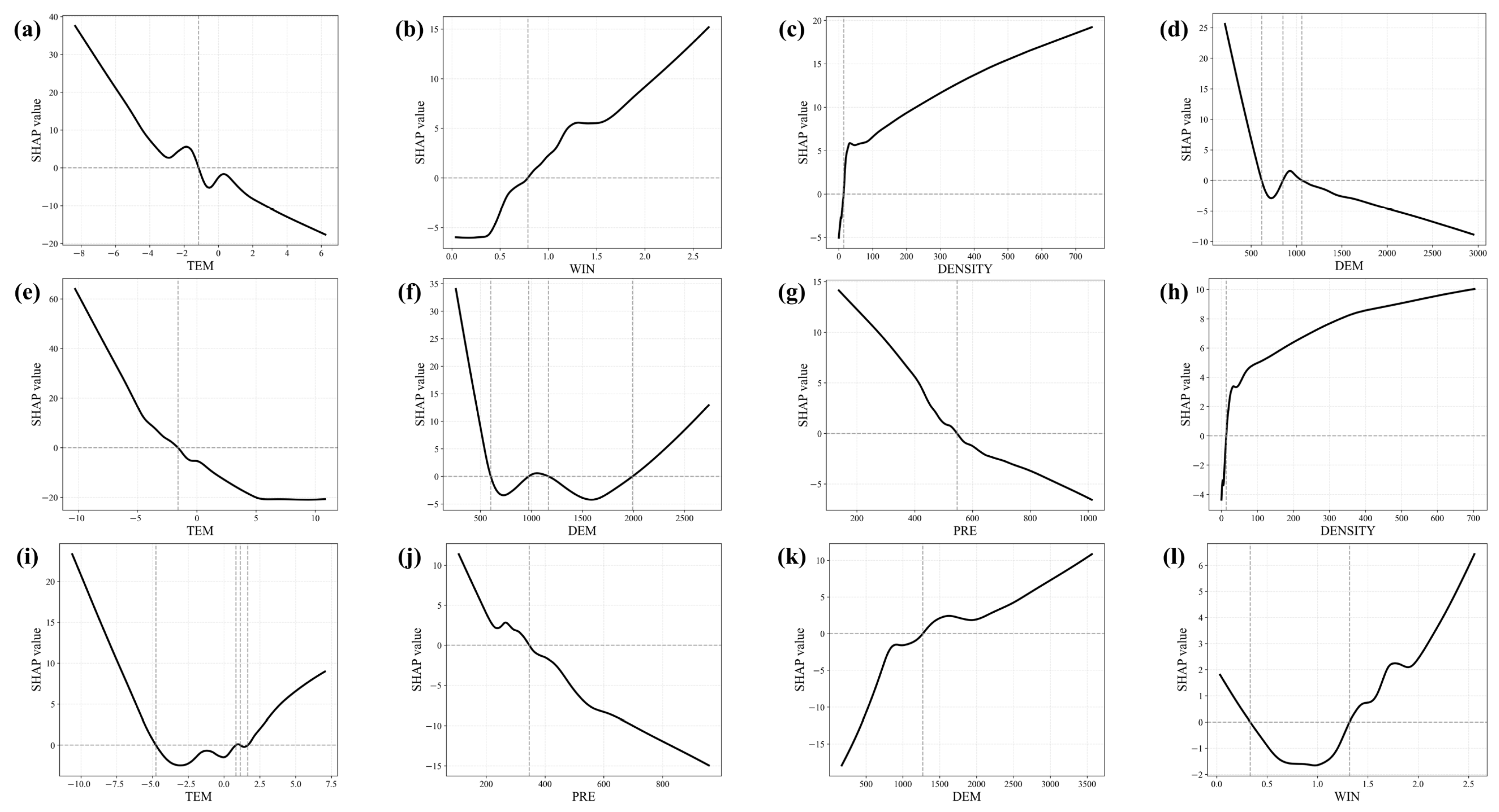
The SHAP dependence plots (Figure 7) reveal significant nonlinear relationships and threshold-like responses between SOS and its associated factors across different vegetation types. Although TEM consistently has the most significant impact on SOS across the three vegetation types, the SOS response curves differ. A linear trend is observed in forests and shrublands, while it is nonlinear in grasslands. For forests (Figure 7a–d), TEM is significantly negatively correlated with SOS. When TEM is below approximately −1 °C, the SHAP value increases rapidly, indicating a significant delaying effect of TEM on SOS under low-temperature conditions. As TEM exceeds −1 °C, this delaying effect gradually transforms into an advancing effect. WIN generally exhibits a positive effect, with a significant increase in SHAP value after approximately 0.8 m/s, indicating that higher wind speeds delay the arrival of SOS. DENSITY is positively correlated with SOS, but its growth rate slows down after approximately 30 heads/hm², and excessively high DENSITY delays SOS. DEM and SOS show a nonlinear negative correlation, fluctuating around 600–100 m. Beyond this range, increased altitude leads to a slight earlier SOS.

For shrubland (Figure 7e–h), TEM also exhibits a strong negative effect, similar to forest, but with a wider response range. A distinct threshold is observed around −2 °C; below this threshold, SOS is significantly delayed. DEM shows a U-shaped relationship, with low SHAP values existing within the 600–2000 m range, indicating that mid-altitude areas may not be conducive to earlier SOS. PRE generally shows a negative correlation, with a threshold around 550 mm. Above this threshold, increased PRE often slightly advances SOS. In contrast, DENSITY shows a positive nonlinear effect; moderate grazing advances SOS, while overgrazing delays it.

For grassland (Figure 7i–l), the nonlinear response is more complex. The TEM exhibits a distinct U-shaped pattern, with its SHAP value reaching a minimum near −3 °C, indicating that both extremely low and high temperatures can delay SOS, while intermediate temperatures can advance it. PRE shows an overall negative impact, with a threshold close to 350 mm, suggesting that insufficient PRE may inhibit early growth. DEM shows a positive correlation, indicating that increasing altitude persistently delays SOS. WIN shows a nonlinear positive correlation, with distinct thresholds around 0.3 °C and 1.3 °C; outside these ranges, windspeed significantly delays SOS.

These results highlight the nonlinear and vegetation-dependent response of SOS to environmental drivers. Temperature remains a major factor, but the form and intensity of its influence vary by vegetation type. The established thresholds further suggest that vegetation responses can abruptly change once environmental conditions exceed certain critical values, emphasizing the importance of considering nonlinear factors.

4. Discussion

4.1. Vegetation-Specific Responses to Environmental Drivers

Although the same environmental variables influence SOS across all vegetation types, their response patterns differ substantially, reflecting contrasting sensitivities to climate change [1]. Forest and shrubland exhibit consistent and significant advancing trends in spring phenology, whereas grassland shows weak and non-significant directional change. This divergence suggests that woody vegetation responds more coherently to interannual climate variability, while grassland phenology is more strongly regulated by limiting environmental conditions [33].

Forests and shrublands are mainly distributed in relatively humid and topographically favorable northern regions, where moisture availability reduces constraints on spring phenological development. In contrast, grasslands occupy more arid southern regions, where water limitation increases the buffering effect of precipitation variability on temperature-driven phenological responses [16].

The contrasting responses can be understood from two geographical perspectives. First, the distribution of vegetation types across the MP follows a clear climatic gradient, with forests and shrublands concentrated in the relatively humid northern mountains and grasslands dominating the drier southern plains. This spatial pattern means that grasslands are inherently subjected to stronger water limitation, making their phenology more sensitive to PRE variability [34]. As PRE plays a crucial role in regulating the temperature dependency of phenology in arid/semiarid regions, the buffered response of forests and shrublands may partly reflect their occupation of more favorable hydrothermal niches [35]. Second, the divergent climate sensitivity reported in recent studies—shrublands showing the highest but declining sensitivity, grasslands exhibiting moderate and increasing sensitivity, and forests maintaining the lowest and most stable sensitivity—indicates that different vegetation types possess distinct capacities to buffer or amplify external climatic signals [36].

The role of human activities further contributes to these differences. Grazing pressure is widely distributed across the plateau and can modulate phenological timing through changes in vegetation structure and soil exposure [37]. However, its influence is likely secondary to climatic controls at the regional scale, particularly in more climatically constrained grassland ecosystems [38]. Moderate grazing may promote earlier SOS by removing standing litter and increasing soil exposure to solar radiation, whereas excessive grazing can delay SOS through soil compaction and reduced vegetation vigor [39,40]. The differing baseline conditions of water availability across vegetation types may further modulate how grazing effects manifest—grasslands, already under greater water stress, may exhibit more complex responses to combined climatic and anthropogenic pressures [41]. Taken together, these findings underscore the importance of incorporating vegetation-specific responses and regional differences when assessing phenological dynamics and formulating ecological management strategies in dryland ecosystems.

4.2. Distinctive Features of Dryland Phenology

The phenological responses observed on the MP are broadly consistent with findings from other dryland and high-latitude ecosystems, yet they also highlight several distinctive features of arid-region phenology.

The advancement of SOS in forest and shrubland aligns with the general pattern of spring phenological acceleration reported across temperate ecosystems in the Northern Hemisphere, indicating a widespread sensitivity of woody vegetation to recent warming [16,42,43]. However, the absence of a significant trend in grassland highlights an important deviation from patterns observed in more mesic grassland systems, where warming typically results in consistent phenological advancement [44,45,46].

This discrepancy likely reflects the dominant role of water limitation in arid and semi-arid ecosystems [47]. In such environments, temperature-driven phenological acceleration can be offset or even suppressed by insufficient moisture availability [48,49]. As a result, grassland phenology is governed by a more complex interaction between thermal and hydrological constraints, making it less responsive to temperature increases alone [50,51,52].

The importance of precipitation and wind-related factors further emphasizes the multi-stressor nature of dryland ecosystems. Compared with energy-limited systems, phenology in the MP is jointly regulated by water availability, atmospheric demand, and surface conditions, which together shape vegetation-specific responses to climate variability [53,54,55].

Nonlinear responses and threshold behaviors further support this interpretation. In water-limited ecosystems, vegetation responses rarely follow linear climate–phenology relationships, and instead exhibit abrupt shifts when environmental conditions exceed critical thresholds [56]. This highlights the importance of considering nonlinear mechanisms when interpreting phenological dynamics in dryland regions.

Finally, the limited independent contribution of human activities in our models, particularly in grasslands, does not imply that grazing and population pressure are ecologically inconsequential. Rather, as noted in previous studies on the MP, the signal of land-use intensity is often statistically confounded with climate variability at regional scales [57,58,59].

4.3. Limitations and Future Work

Despite the insights gained from this study, several limitations must be acknowledged, which also point toward promising directions for future research. First, uncertainty is inherent in the extraction of SOS from NDVI time series. The 16-day compositing interval of MOD13Q1, although suitable for regional-scale monitoring, may obscure subtle phenological transitions, particularly in sparsely vegetated areas where soil background effects are pronounced [60,61]. Moreover, the fixed 20% dynamic threshold employed here, while widely used in phenological studies, does not account for interannual variations in the shape of the NDVI seasonal curve, which may shift under extreme climatic conditions [62]. Second, the spatial resolution of certain driving factor datasets constrains the analysis. The ERA5-Land climate variables have a native resolution of approximately 11 km, which may inadequately resolve fine-scale topographic and microclimatic influences on phenology, especially in mountainous terrain. Third, the modeling framework employed in this study, while powerful for detecting nonlinear relationships, has inherent limitations in causal inference. XGBoost quantifies predictor importance but does not establish causality. Although SHAP analysis mitigates this issue by isolating marginal contributions, residual confounding cannot be entirely eliminated. The U-shaped temperature response identified for grasslands, though ecologically plausible, requires further validation through controlled field experiments or process-based simulations that explicitly represent the physiological mechanisms underlying such threshold behavior. Fourth, the analysis was restricted to areas where land cover remained stable throughout the 2001–2020 period. This design effectively isolates phenological signals from the confounding effects of land-use change, but it also excludes regions undergoing active transformation, such as cropland expansion, urbanization, or vegetation degradation. The phenological responses documented here may therefore represent a relatively conservative signal, and the full magnitude of human-induced phenological shifts across the MP could be underestimated.

Building on these limitations, several directions for future research emerge. Higher temporal resolution remote sensing data, combined with adaptive thresholding techniques, could improve the accuracy of SOS detection in heterogeneous dryland landscapes. Integrating field-based grazing intensity surveys and high-resolution animal tracking data would help disentangle the true ecological role of herbivory from statistical artifacts associated with coarse spatial datasets. Furthermore, coupling machine learning approaches with process-based phenological models offers a promising pathway to move beyond predictive importance toward mechanistic understanding, particularly for the nonlinear threshold behaviors revealed in this study. Finally, extending the analytical domain to include transitional and human-modified landscapes would provide a more comprehensive assessment of how climate forcing and land-surface changes jointly shape vegetation phenology across the MP.

5. Conclusions

Based on the analysis of MODIS-derived SOS from 2001 to 2020 across stable vegetation areas of the MP, this study revealed pronounced spatial heterogeneity in spring phenology trends. Forest and shrubland ecosystems in the northern and northeastern mountainous regions exhibited significant advancing trends, with mean SOS occurring at approximately 107 DOY and advancing by 6.8 and 6.4 days per decade, respectively. In contrast, grassland ecosystems, which dominate the southern and southwestern arid regions, displayed a later mean SOS (138 DOY) and no significant temporal trend, with localized delays exceeding 0.8 days per year along the desert–steppe transition zone. After excluding non-significant areas, 65.4% of the remaining region showed advancing SOS while 34.6% exhibited delaying trends. Temperature consistently emerged as the dominant driver across all vegetation types, yet its relative importance and response form varied substantially. SHAP analysis further identified strong nonlinearities, including a U-shaped temperature response and a precipitation threshold near 350 mm in grasslands, as well as windspeed and livestock density thresholds in forests. These findings underscore the vegetation-specific and nonlinear nature of phenological regulation in drylands, providing a more mechanistic basis for projecting ecosystem responses to climate change. They also highlight the importance of incorporating region- and vegetation-specific thresholds into ecological management and climate adaptation strategies, particularly in the water-limited grasslands and wind-exposed forests of the MP, where divergent phenological sensitivities may have cascading implications for carbon cycling, forage availability, and ecosystem stability.

References

1. Piao, S.; Liu, Q.; Chen, A.; Janssens, I.A.; Fu, Y.; Dai, J.; Liu, L.; Lian, X.; Shen, M.; Zhu, X. Plant Phenology and Global Climate Change: Current Progresses and Challenges. Glob. Change Biol. 2019, 25, 1922–1940. [Google Scholar] [CrossRef]
2. Keenan, T.F.; Gray, J.; Friedl, M.A.; Toomey, M.; Bohrer, G.; Hollinger, D.Y.; Munger, J.W.; O’Keefe, J.; Schmid, H.P.; Wing, I.S.; et al. Net Carbon Uptake Has Increased through Warming-Induced Changes in Temperate Forest Phenology. Nat. Clim. Change 2014, 4, 598–604. [Google Scholar] [CrossRef]
3. Richardson, A.D.; Keenan, T.F.; Migliavacca, M.; Ryu, Y.; Sonnentag, O.; Toomey, M. Climate Change, Phenology, and Phenological Control of Vegetation Feedbacks to the Climate System. Agric. For. Meteorol. 2013, 169, 156–173. [Google Scholar] [CrossRef]
4. Miao, L.; Liu, Q.; Fraser, R.; He, B.; Cui, X. Shifts in Vegetation Growth in Response to Multiple Factors on the Mongolian Plateau from 1982 to 2011. Phys. Chem. Earth Parts A/B/C 2015, 87–88, 50–59. [Google Scholar] [CrossRef]
5. Morante-Carballo, F.; Montalván-Burbano, N.; Quiñonez-Barzola, X.; Jaya-Montalvo, M.; Carrión-Mero, P. What Do We Know about Water Scarcity in Semi-Arid Zones? A Global Analysis and Research Trends. Water 2022, 14, 2685. [Google Scholar] [CrossRef]
6. Zhao, J.; Yu, Q.; Avirmed, B.; Wang, Y.; Orgilbold, M.; Cui, H.; Liu, Y.; Lian, J. The Relationship between Structure and Ecosystem Services of Forest and Grassland Based on Pattern Analysis Method: A Case Study of the Mongolian Plateau. Sci. Total Environ. 2024, 948, 174700. [Google Scholar] [CrossRef] [PubMed]
7. Miao, L.; Sun, Z.; Ren, Y.; Schierhorn, F.; Müller, D. Grassland Greening on the Mongolian Plateau despite Higher Grazing Intensity. Land Degrad. Dev. 2021, 32, 792–802. [Google Scholar] [CrossRef]
8. Yan, Y.; Cheng, Y.; Xin, Z.; Zhou, J.; Zhou, M.; Wang, X. Impacts of Climate Change and Human Activities on Vegetation Dynamics on the Mongolian Plateau, East Asia from 2000 to 2023. J. Arid Land 2024, 16, 1062–1079. [Google Scholar] [CrossRef]
9. Li, B.; Wang, R.; Chen, J.M. Responses of Phenology to Preseason Drought and Soil Temperature for Different Land Cover Types on the Mongolian Plateau. Sci. Total Environ. 2024, 926, 171895. [Google Scholar] [CrossRef]
10. Li, C.; Wang, R.; Cui, X.; Wu, F.; Yan, Y.; Peng, Q.; Qian, Z.; Xu, Y. Responses of Vegetation Spring Phenology to Climatic Factors in Xinjiang, China. Ecol. Indic. 2021, 124, 107286. [Google Scholar] [CrossRef]
11. Li, Q.; Gao, X.; Li, J.; Yan, A.; Chang, S.; Song, X.; Lo, K. Nonlinear Time Effects of Vegetation Response to Climate Change: Evidence from Qilian Mountain National Park in China. Sci. Total Environ. 2024, 933, 173149. [Google Scholar] [CrossRef]
12. Iler, A.M.; Høye, T.T.; Inouye, D.W.; Schmidt, N.M. Nonlinear Flowering Responses to Climate: Are Species Approaching Their Limits of Phenological Change? Philos. Trans. R. Soc. Lond. B Biol. Sci. 2013, 368, 20120489. [Google Scholar] [CrossRef]
13. Caparros-Santiago, J.A.; Rodriguez-Galiano, V.; Dash, J. Land Surface Phenology as Indicator of Global Terrestrial Ecosystem Dynamics: A Systematic Review. ISPRS J. Photogramm. Remote Sens. 2021, 171, 330–347. [Google Scholar] [CrossRef]
14. Lü, J.; Wang, R.; Sardans, J.; Peñuelas, J.; Jiang, Y.; Han, X. An Integrative Review of Drivers and Responses of Grassland Phenology under Global Change. Crit. Rev. Plant Sci. 2023, 42, 124–137. [Google Scholar] [CrossRef]
15. Estefania-Salazar, E.; Iglesias, E. Assessing Vegetation Phenology Dynamics in West African Rangelands: Implications for Livestock Sustainability and Transhumance. Ecol. Inform. 2025, 88, 103138. [Google Scholar] [CrossRef]
16. Zhang, X.; Jia, W.; Li, Y.; Luo, L.; Atkinson, P. Comparative Analysis of Long-Term Trends and Climate Sensitivity of Spring Phenology across Forests, Shrublands, and Grasslands in the Middle–High Latitudes of the Northern Hemisphere. GISci. Remote Sens. 2025, 62, 2572165. [Google Scholar] [CrossRef]
17. Baudena, M.; Dekker, S.C.; van Bodegom, P.M.; Cuesta, B.; Higgins, S.I.; Lehsten, V.; Reick, C.H.; Rietkerk, M.; Scheiter, S.; Yin, Z.; et al. Forests, Savannas, and Grasslands: Bridging the Knowledge Gap between Ecology and Dynamic Global Vegetation Models. Biogeosciences 2015, 12, 1833–1848. [Google Scholar] [CrossRef]
18. Dulamsuren, C.; Hauck, M.; Muhlenberg, M. Vegetation at the Taiga Forest-Steppe Borderline in the Western Khentey Mountains, Northern Mongolia. Ann. Bot. Fenn. 2005, 42, 411–426. [Google Scholar]
19. Bai, Y.; Xu, Z.; Li, D. On the Small Scale Spatial Heterogeneity of Soil Moisture, Carbon and Nitrogen in Stipa Communities of the Inner Mongolia Plateau. Acta Ecol. Sin. 2002, 22, 1215–1223. [Google Scholar]
20. Zhao, Z.; Lu, C.; Tonooka, H.; Wu, L.; Lin, H.; Jiang, X. Dynamic Monitoring of Vegetation Phenology on the Qinghai-Tibetan Plateau from 2001 to 2020 via the MSAVI and EVI. Sci. Rep. 2025, 15, 25698. [Google Scholar] [CrossRef]
21. Huang, X.; Liu, J.; Zhu, W.; Atzberger, C.; Liu, Q. The Optimal Threshold and Vegetation Index Time Series for Retrieving Crop Phenology Based on a Modified Dynamic Threshold Method. Remote Sens. 2019, 11, 2725. [Google Scholar] [CrossRef]
22. Li, H.; Li, F.Y.; Guo, J.; Gao, X. An Improved Dynamic Threshold Method for Determining the Start of the Vegetation Greening Season in Remote Sensing Monitoring: The Case of Inner Mongolia. Ecol. Inform. 2023, 78, 102378. [Google Scholar] [CrossRef]
23. Li, N.; Zhan, P.; Pan, Y.; Zhu, X.; Li, M.; Zhang, D. Comparison of Remote Sensing Time-Series Smoothing Methods for Grassland Spring Phenology Extraction on the Qinghai–Tibetan Plateau. Remote Sens. 2020, 12, 3383. [Google Scholar] [CrossRef]
24. Gong, Z.; Ge, W.; Guo, J.; Liu, J. Satellite Remote Sensing of Vegetation Phenology: Progress, Challenges, and Opportunities. ISPRS J. Photogramm. Remote Sens. 2024, 217, 149–164. [Google Scholar] [CrossRef]
25. Sen, P.K. Estimates of the Regression Coefficient Based on Kendall’s Tau. J. Am. Stat. Assoc. 1968, 63, 1379–1389. [Google Scholar] [CrossRef]
26. Mann, H.B. Nonparametric Tests against Trend. Econometrica 1945, 13, 245–259. [Google Scholar] [CrossRef]
27. Kendall, M.G. Rank Correlation Methods, 4th ed.; 2d impression.; Griffin: London, UK, 1975; ISBN 978-0-85264-199-6. [Google Scholar]
28. Meng, X.; Gao, X.; Li, S.; Lei, J. Spatial and Temporal Characteristics of Vegetation NDVI Changes and the Driving Forces in Mongolia during 1982–2015. Remote Sens. 2020, 12, 603. [Google Scholar] [CrossRef]
29. Chan, J.Y.-L.; Leow, S.M.H.; Bea, K.T.; Cheng, W.K.; Phoong, S.W.; Hong, Z.-W.; Chen, Y.-L. Mitigating the Multicollinearity Problem and Its Machine Learning Approach: A Review. Mathematics 2022, 10, 1283. [Google Scholar] [CrossRef]
30. Chen, T.; Guestrin, C. XGBoost: A Scalable Tree Boosting System. In Proceedings of the 22nd ACM SIGKDD International Conference on Knowledge Discovery and Data Mining; Association for Computing Machinery: New York, NY, USA, 2016; pp. 785–794. [Google Scholar]
31. Delaney, J.T.; Larson, D.M. Using Explainable Machine Learning Methods to Evaluate Vulnerability and Restoration Potential of Ecosystem State Transitions. Conserv. Biol. 2024, 38, e14203. [Google Scholar] [CrossRef]
32. Lundberg, S.M.; Lee, S.-I. A Unified Approach to Interpreting Model Predictions. In Proceedings of the Advances in Neural Information Processing Systems; Curran Associates, Inc.: New York, NY, USA, 2017; Volume 30. [Google Scholar]
33. Zhao, X.; Hu, H.; Shen, H.; Zhou, D.; Zhou, L.; Myneni, R.B.; Fang, J. Satellite-Indicated Long-Term Vegetation Changes and Their Drivers on the Mongolian Plateau. Landsc. Ecol. 2015, 30, 1599–1611. [Google Scholar] [CrossRef]
34. Miao, L.; Müller, D.; Cui, X.; Ma, M. Changes in Vegetation Phenology on the Mongolian Plateau and Their Climatic Determinants. PLoS ONE 2017, 12, e0190313. [Google Scholar] [CrossRef]
35. Snyder, K.A.; Tartowski, S.L. Multi-Scale Temporal Variation in Water Availability: Implications for Vegetation Dynamics in Arid and Semi-Arid Ecosystems. J. Arid. Environ. 2006, 65, 219–234. [Google Scholar] [CrossRef]
36. Currier, C.M.; Sala, O.E. Precipitation versus Temperature as Phenology Controls in Drylands. Ecology 2022, 103, e3793. [Google Scholar] [CrossRef]
37. Liang, Y.; Han, G.; Zhou, H.; Zhao, M.; Snyman, H.A.; Shan, D.; Havstad, K.M. Grazing Intensity on Vegetation Dynamics of a Typical Steppe in Northeast Inner Mongolia. Rangel. Ecol. Manag. 2009, 62, 328–336. [Google Scholar] [CrossRef]
38. Wang, L.; Jiao, W.; MacBean, N.; Rulli, M.C.; Manzoni, S.; Vico, G.; D’Odorico, P. Dryland Productivity under a Changing Climate. Nat. Clim. Change 2022, 12, 981–994. [Google Scholar] [CrossRef]
39. Balata, D.; Gama, I.; Domingos, T.; Proença, V. Using Satellite NDVI Time-Series to Monitor Grazing Effects on Vegetation Productivity and Phenology in Heterogeneous Mediterranean Forests. Remote Sens. 2022, 14, 2322. [Google Scholar] [CrossRef]
40. Berisha, N.; Geci, D. The Analysis of the Influence of Grazing Intensity on the Diversity and Abundance of Plants and Spiders (Arachnida: Araneae). Eur. J. Environ. Sci. 2023, 13, 31–38. [Google Scholar] [CrossRef]
41. Godde, C.; Dizyee, K.; Ash, A.; Thornton, P.; Sloat, L.; Roura, E.; Henderson, B.; Herrero, M. Climate Change and Variability Impacts on Grazing Herds: Insights from a System Dynamics Approach for Semi-Arid Australian Rangelands. Glob. Change Biol. 2019, 25, 3091–3109. [Google Scholar] [CrossRef] [PubMed]
42. Jeong, S.-J.; Ho, C.-H.; Gim, H.-J.; Brown, M.E. Phenology Shifts at Start vs. End of Growing Season in Temperate Vegetation over the Northern Hemisphere for the Period 1982–2008. Glob. Change Biol. 2011, 17, 2385–2399. [Google Scholar] [CrossRef]
43. Lian, X.; Piao, S.; Chen, A.; Wang, K.; Li, X.; Buermann, W.; Huntingford, C.; Peñuelas, J.; Xu, H.; Myneni, R.B. Seasonal Biological Carryover Dominates Northern Vegetation Growth. Nat. Commun. 2021, 12, 983. [Google Scholar] [CrossRef]
44. Chen, H.; Zhao, J.; Zhang, H.; Zhang, Z.; Guo, X.; Wang, M. Detection and Attribution of the Start of the Growing Season Changes in the Northern Hemisphere. Sci. Total Environ. 2023, 903, 166607. [Google Scholar] [CrossRef] [PubMed]
45. Ren, S.; Chen, X.; Lang, W.; Schwartz, M.D. Climatic Controls of the Spatial Patterns of Vegetation Phenology in Midlatitude Grasslands of the Northern Hemisphere. J. Geophys. Res. Biogeosci. 2018, 123, 2323–2336. [Google Scholar] [CrossRef]
46. Karthe, D.; Chalov, S.; Gradel, A.; Kusbach, A. Special Issue «environment Change on the Mongolian Plateau: Atmosphere, Forests, Soils and Water». Geogr. Environ. Sustain. 2019, 12, 60–65. [Google Scholar] [CrossRef][Green Version]
47. Luo, Y.; Yang, H.; Xu, H.; Huntingford, C.; Orth, R.; Li, X.; Peñuelas, J. Concurrent Climate Extremes and Biological Carryover Effects Dominate Severe Seasonal Reductions in Northern Vegetation Growth. One Earth 2026, 9, 101624. [Google Scholar] [CrossRef]
48. Li, R.; Luo, T.; Mölg, T.; Zhao, J.; Li, X.; Cui, X.; Du, M.; Tang, Y. Leaf Unfolding of Tibetan Alpine Meadows Captures the Arrival of Monsoon Rainfall. Sci. Rep. 2016, 6, 20985. [Google Scholar] [CrossRef]
49. Shen, M.; Piao, S.; Cong, N.; Zhang, G.; Jassens, I.A. Precipitation Impacts on Vegetation Spring Phenology on the Tibetan Plateau. Glob. Change Biol. 2015, 21, 3647–3656. [Google Scholar] [CrossRef]
50. Fu, Y.H.; Piao, S.; Zhao, H.; Jeong, S.-J.; Wang, X.; Vitasse, Y.; Ciais, P.; Janssens, I.A. Unexpected Role of Winter Precipitation in Determining Heat Requirement for Spring Vegetation Green-Up at Northern Middle and High Latitudes. Glob. Change Biol. 2014, 20, 3743–3755. [Google Scholar] [CrossRef]
51. Cui, T.; Martz, L.; Guo, X. Grassland Phenology Response to Drought in the Canadian Prairies. Remote Sens. 2017, 9, 1258. [Google Scholar] [CrossRef]
52. Yuan, Z.; Bao, G.; Dorjsuren, A.; Oyont, A.; Chen, J.; Li, F.; Dong, G.; Guo, E.; Shao, C.; Du, L. Climatic Constraints of Spring Phenology and Its Variability on the Mongolian Plateau from 1982 to 2021. J. Geophys. Res. Biogeosciences 2024, 129, e2023JG007689. [Google Scholar] [CrossRef]
53. Dong, L.; Wu, C.; Wang, X.; Zhao, N. Satellite Observed Delaying Effects of Increased Winds on Spring Green-Up Dates. Remote Sens. Environ. 2023, 284, 113363. [Google Scholar] [CrossRef]
54. Zhang, S.; Liu, G.; Cui, Q.; Huang, Z.; Ye, X.; Cornelissen, J.H.C. New Field Wind Manipulation Methodology Reveals Adaptive Responses of Steppe Plants to Increased and Reduced Wind Speed. Plant Methods 2021, 17, 5. [Google Scholar] [CrossRef]
55. Meng, X.; Ling, Z.; Chen, Y.; Kuang, J.; Zhang, L.; Wu, Z.; Zheng, Z.; Wang, J. From Coast to Inland: Nonlinear and Temperature-Mediated Urbanization Effects on Vegetation Phenology in Shandong Province, China. Remote Sens. 2025, 17, 3833. [Google Scholar] [CrossRef]
56. Mei, L.; Bao, G.; Tong, S.; Yin, S.; Bao, Y.; Jiang, K.; Hong, Y.; Tuya, A.; Huang, X. Elevation-Dependent Response of Spring Phenology to Climate and Its Legacy Effect on Vegetation Growth in the Mountains of Northwest Mongolia. Ecol. Indic. 2021, 126, 107640. [Google Scholar] [CrossRef]
57. Xiao, X.; Wang, Q.; Guan, Q.; Zhang, Z.; Yan, Y.; Mi, J.; Yang, E. Quantifying the Nonlinear Response of Vegetation Greening to Driving Factors in Longnan of China Based on Machine Learning Algorithm. Ecol. Indic. 2023, 151, 110277. [Google Scholar] [CrossRef]
58. Dutra, A.C.; Srivastava, A.; Ganem, K.A.; Arai, E.; Huete, A.; Shimabukuro, Y.E. Remote Sensing-Based Phenology of Dryland Vegetation: Contributions and Perspectives in the Southern Hemisphere. Remote Sens. 2025, 17, 2503. [Google Scholar] [CrossRef]
59. AghaKouchak, A.; Farahmand, A.; Melton, F.S.; Teixeira, J.; Anderson, M.C.; Wardlow, B.D.; Hain, C.R. Remote Sensing of Drought: Progress, Challenges and Opportunities. Rev. Geophys. 2015, 53, 452–480. [Google Scholar] [CrossRef]
60. Zhang, X.; Friedl, M.A.; Schaaf, C.B. Sensitivity of Vegetation Phenology Detection to the Temporal Resolution of Satellite Data. Int. J. Remote Sens. 2009, 30, 2061–2074. [Google Scholar] [CrossRef]
61. Tan, B.; Friedl, M.; Zhang, X. Challenges in Estimating the Vegetation Phenology with Remote Sensed Data. In AGU Fall Meeting Abstracts; American Geophysical Union: Washington, DC, USA, 2006; Volume 2006. [Google Scholar]
62. Pohl, M.J.; Lehnert, L.; Thies, B.; Seeger, K.; Berdugo, M.B.; Gradstein, S.R.; Bader, M.Y.; Bendix, J. Downscaling Air Temperatures for High-Resolution Niche Modeling in a Valley of the Amazon Lowland Forests: A Case Study on the Microclima R Package. PLoS ONE 2024, 19, e0310423. [Google Scholar] [CrossRef]
Figure 1. Location of the study area (a), elevation of the MP (b), vegetation cover types derived from the MODIS Land Cover Product (MCD12Q1, IGBP) (c) and extent of the vegetation phenology monitoring area (d).
Land 15 00790 g001
Figure 2. Spatial distribution and temporal trends of the SOS. Spatial distribution maps of the SOS for 2001, 2005, 2010, 2015, and 2020 (ae). Temporal variation in the annual mean SOS (f).
Land 15 00790 g002
Figure 3. SOS Trend Analysis. Spatial distribution of SOS slope estimator β values from 2001 to 2020 (a), spatial distribution of SOS MK test Z values from 2001 to 2020 (b), spatial distribution of SOS trends from 2001 to 2020 (c).
Land 15 00790 g003
Figure 4. Trends in SOS across Different Vegetation Cover Regions from 2001 to 2020.
Land 15 00790 g004
Figure 5. Distribution of SOS in different vegetation cover regions from 2001 to 2020.
Land 15 00790 g005
Figure 6. The importance of SOS drivers for forests (a), shrubs (b), and grasses (c).
Land 15 00790 g006
Figure 7. SHAP dependence plots of SOS drivers in the forest (ad), SHAP dependence plots of SOS drivers in the shrubs (eh), SHAP dependence plots of SOS drivers in the grasses (il).
Land 15 00790 g007