Machine Learning-Based Bioclimatic Suitability Modeling for Maize Cultivation Under Future Projections

Abstract

Climate-driven heat and water stress are increasingly compromising rainfed maize yields in transition zones, with significant implications for global food security. While continental-scale models of crop suitability exist, they often fail to capture the high-resolution heterogeneity of agricultural landscapes or distinguish between irrigated and rainfed systems in semi-arid regions. This study models the current and future suitability of rainfed maize in Kansas, USA, using a Maximum Entropy (MaxEnt) approach. To accurately isolate biophysical constraints, we employed a novel data-filtering workflow using the USDA Cropland Data Layer (CDL) and Landsat-based Annual Irrigated Datasets (LANID) to train the model exclusively on rainfed occurrences. We projected suitability shifts for the mid- (2041–2070) and end-of-century (2071–2100) periods under two CMIP6 Shared Socioeconomic Pathways (SSP3-7.0 and SSP5-8.5), using high-resolution CHELSA bioclimatic variables. The model, achieving an Area Under the Curve (AUC) of 0.73 and validated against 30 years of historical USDA production records, reveals a distinct spatial contraction of areas climatically suitable for growing maize. Projections indicate a significant decline in suitability across Western and Central Kansas driven by rising temperatures and precipitation variability, with the most highly suitable optimal habitats projected to decline by approximately 90% by mid-century. These findings quantify mounting climate impacts on maize-growing areas of the Great Plains and provide spatially explicit baselines for the development of regional adaptation strategies and groundwater conservation policies.

1. Introduction

Maize (Zea mays L.) is a vital global crop, playing a crucial role in food security and economic stability in many regions [1,2,3]. However, climate change poses serious risks to its sustainable production due to rising temperatures, shifting precipitation patterns, and more frequent extreme weather events [1,4]. The United States faces potential yield losses of 10.3% (±5.4%) per degree Celsius of warming [5] and is expected to see a sharp decrease in the land area considered “optimally suitable” for maize cultivation, with reductions ranging from 17.16% to 42.91% depending on the future climate scenario [4]. Therefore, reliable modeling of maize cultivation suitability under future climate conditions has become a critical priority for engineers, agronomists, policymakers, and farmers [6,7].

The sensitivity of maize to climatic variables is well documented, making the selection of predictors critical for modeling. Temperature strongly influences crop phenology from germination to maturity [8], where excessive heat accumulation can shorten the grain-filling period and reduce yields [9]. Specifically, temperatures exceeding 29–30 °C during flowering can cause sharp yield losses [10,11]. Under rainfed farming systems, maize is heavily constrained by water availability, making it vulnerable to the dual threats of drought and precipitation variability [8,12]. Understanding these biophysical constraints is essential for accurately projecting future spatial suitability for growing maize, as physiological traits and site-specific environmental factors have been shown to significantly modulate plant-water fluxes across varying climate regimes [13].

To anticipate and mitigate these risks, researchers frequently employ species distribution models (SDMs) to predict shifts in crop suitability [14,15]. Among these, the maximum entropy (MaxEnt) approach has emerged as a powerful tool. Unlike mechanistic crop models, which require extensive physiological calibration data, MaxEnt is highly valued for its ability to generate robust predictions using only “presence” data—locations where the crop is known to grow—without requiring reliable true absence data [16].

In agricultural contexts, proving true absence is difficult because a crop might not be grown in a specific location due to socio-economic factors (e.g., land use choices, market access) rather than environmental unsuitability [16]. Accordingly, MaxEnt was preferred over discriminative machine learning models, such as Random Forest and Support Vector Machines, because these methods generally depend on reliable true absence data, whereas MaxEnt applies a presence-background approach. Theoretically, MaxEnt estimates the relative likelihood of presence across environmental gradients by minimizing the relative entropy between the probability density of species occurrence and that of the environmental background [17,18]. Following this well-established method, numerous studies have successfully mapped current and future suitability for various crops [6,19].

Despite this body of work, critical gaps remain in the regional application of these models. While large-scale spatial baselines exist [16], they often lack the resolution to capture the nuances of heterogeneous agricultural landscapes. Located in the geographic center of the contiguous United States, the State of Kansas serves as a unique and scientifically significant case study of a climatic “transition zone”. The state is characterized by a significant topographical gradient, with elevation rising from 679 feet (207 m) in the southeast to 4039 feet (1231 m) at the western border [20]. This topography drives a steep precipitation gradient—ranging from over 45 inches (1,140 mm) in the humid subtropical southeast to less than 20 inches (500 mm) in the semi-arid high plains of the west [21]—making it an ideal laboratory for observing the “front lines” of climate-induced agricultural shifts. This southwest-to-northeast precipitation pattern is strongly influenced by storm systems moving northeast from the Gulf of Mexico, producing marked spatial variation in annual precipitation across Kansas. Although elevation and temperature gradients also shape environmental variability, precipitation amounts and seasonality remain the primary constraints on the “presence” of rainfed maize in Kansas. Moreover, spatial soil variability in the region strongly influences effective water availability by regulating infiltration and root-zone storage; accordingly, the suitability maps developed here should be interpreted as representing climatic suitability [22,23].

These intersecting gradients create three major Köppen climate classifications: a humid subtropical (Cfa) zone in the southeast, a large humid continental (Dfa) zone across the central and northeastern regions, and a cold semi-arid steppe (BSk) zone in the western third [24]. Consequently, Kansas features diverse agro-ecological conditions, ranging from primarily rainfed systems in the east to irrigation-dependent agriculture in the west.

Despite this environmental variability, Kansas remains a nationally significant center for maize production. According to the USDA’s National Agricultural Statistics Service, 6.3 million acres were planted with corn in 2024, yielding 748.2 million bushels at an average of 129 bushels per acre [25]. This high level of production, particularly in the semi-arid western regions, underscores both the crop’s economic significance and its deep reliance on regional water resources.

These transition zones act as the “new 100th meridian”, marking the volatile boundary where aridity is shifting eastward into previously productive rainfed regions [26]. Such areas are characterized by heightened sensitivity to precipitation deficits, in which rainfed maize lacks the thermal buffering capacity provided by irrigation—effectively lowering its extreme-heat threshold from approximately 35 °C to 32 °C. Consequently, the reliance on finite groundwater resources to maintain production in these shifting zones creates a sustainability paradox that broad-scale models often overlook [16].

The urgency of accurate modeling in this transition zone is underscored by recent local projections. In the Eastern Kansas River Basin, a vital rainfed agricultural region, maize yield losses are projected to range from 23% to 34% by the end of the century under intermediate emissions (RCP 4.5) and 36% to 57% under high emissions (RCP 8.5). For the mid-century period (2040–2069), losses are projected between 11% and 22% (RCP 4.5) and 22% and 38% (RCP 8.5) [26].

Current broad-scale studies fail to capture how the specific environmental gradient driving these losses will migrate under distinct climate futures. Moreover, few studies have charted the progressive shifts in maize suitability across multiple future time periods (mid vs. end of the century) using the most recent CMIP6 Shared Socioeconomic Pathways (SSPs), leaving uncertainty about the temporal velocity of these changes.

To address these gaps, this study provides a comprehensive forecast of the suitability of rainfed maize cultivation in Kansas by employing a novel masking approach to isolate strict biophysical constraints from artificial irrigation buffers. Using a MaxEnt modeling approach, we analyze the impacts of climate change under two distinct SSPs (SSP3-7.0 and SSP5-8.5). Specifically, we aim to: (1) quantify the projected changes in the location of areas suitable for rainfed maize over time; (2) identify key bioclimatic variables that are primary limiting factors for cultivation in the region; and (3) provide spatially explicit maps that can potentially help regional stakeholders in developing climate adaptation strategies.

2. Methods

This study employs a comprehensive species distribution modeling (SDM) framework to assess the current suitability and forecast future suitability for maize. The workflow is designed to ensure methodological transparency, statistical robustness, and replicability, addressing known challenges in large-scale agricultural suitability modeling, including data quality, sampling bias, and uncertainty in future climate projections. The framework encompasses four stages: (1) acquisition and rigorous pre-processing of global species occurrence records and high-resolution environmental data; (2) systematic parameterization and optimization of a Maximum Entropy (MaxEnt) model to identify the most parsimonious and predictive model structure; (3) robust model evaluation using spatial cross-validation and threshold-independent performance metrics; and (4) projection of the optimized model onto an ensemble of future climate scenarios to quantify the potential range and uncertainty of shifts in suitable habitat.

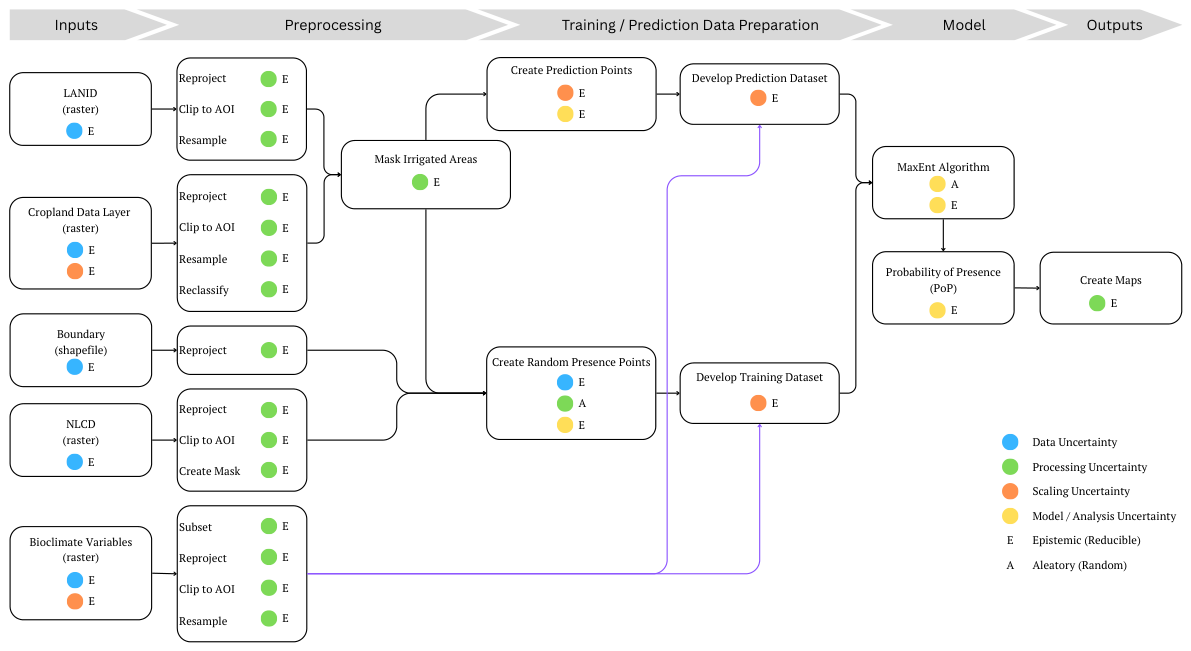
Figure 1 provides a detailed flowchart of this methodology, illustrating the flow of data from initial inputs (e.g., boundary files, NLCD, and climate data) through all preprocessing, data preparation, and modeling steps to the final probability of presence maps.

The foundation of any reliable species distribution model is the quality of its input data. The outcome of a model is only as sound as the data used to construct it, a principle that necessitates meticulous data curation and bias correction. This initial phase of the study focuses on assembling comprehensive datasets for both species occurrences and environmental predictors.

Table 1. Dataset Summary and Processing Steps.

Dataset Name	Year	Data Format and Resolution	Project CRS (EPSG)	Area (km2)
Kansas State Boundary (AOI *)	2020	Vector (Polyline)	26,914	Total Area: 213,121
USDA NASS Cropland Data Layer (CDL)	2024	Raster (30 m)	26,914	Total Maize Land: 24,991
Landsat-based Annual Irrigated Datasets (LANID)	2020	Raster (30 m)	26,914	Total Irrigated Land in AOI: 12,494
Rainfed Maize Dataset	Derived	Raster (180 m)	26,914	Rainfed Maize Area: 19,436
USGS National Land Cover Database (NLCD)	2021	Raster (30 m)	26,914	Viable Agricultural Land: 96,529 (Mask)
Presence Points	n/a	Vector (Point)	26,914	n/a
Prediction Points	n/a	Vector (Point)	26,914	n/a
CHELSA bioclimate variables (BIO1–BIO19)	1981–2010 (baseline); 2041–2070 (mid-century); 2071–2100 (end-of-century)	Raster (∼1 km)	26,914	n/a
USDA county production data (validation)	1981–2010	Tabular by county	n/a	n/a

* AOI: Area of Interest.

summarizes the scope of these datasets, detailing their native resolutions and the specific processing criteria used to align them within the Kansas modeling domain.

2.1. Study Area

The modeling domain encompasses the state of Kansas. The vector boundary of the state [27] was used as the definitive spatial extent to clip all predictor variables and mask subsequent model predictions. To ensure spatial alignment and accurate geometric calculations, all geospatial datasets—including occurrence records and environmental predictors—were reprojected to the NAD 1983 UTM Zone 14N (EPSG: 26914) coordinate reference system.

2.2. Maize Occurrence Records

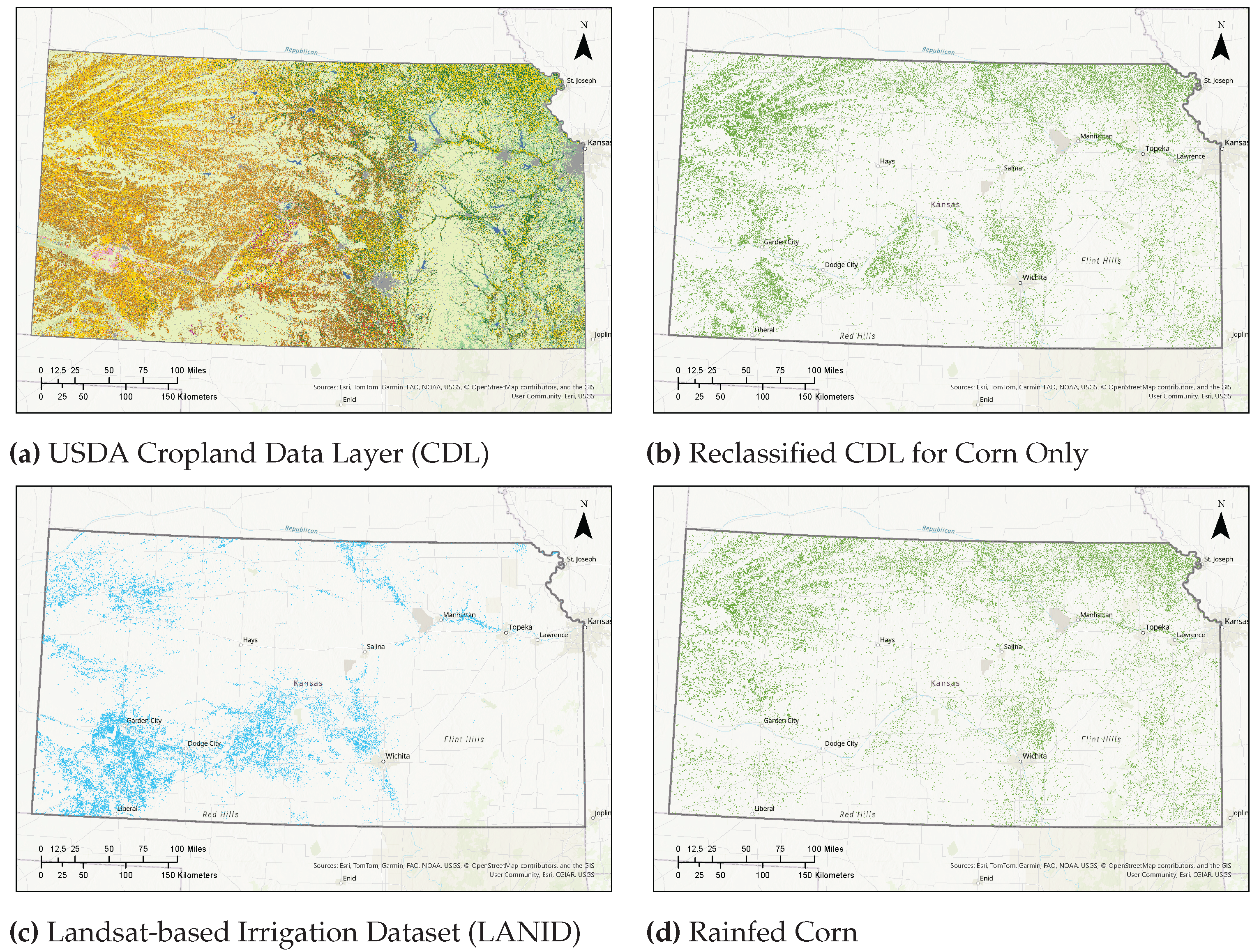
Maize occurrences were derived from the USDA National Agricultural Statistics Service (NASS) Cropland Data Layer (CDL) 2024, a highly accurate, 30-m resolution satellite-based land cover product [28] (Figure 2a). To match the spatial resolution of the environmental predictor variables, the native CDL raster for Kansas was resampled to 180 m using the nearest neighbor method. The dataset was subsequently reclassified into a binary layer, isolating maize occurrences from all other land cover types (Figure 2b). This binary raster served as the foundational presence data for the distribution model.

2.3. Isolation of Rainfed Maize Occurrences

Because this study utilizes bioclimatic variables as the sole predictors of suitability, including irrigated lands in the training data would introduce significant bias by artificially inflating climatic suitability in low-precipitation zones. Irrigation can decouple maize presence from local precipitation constraints, particularly in western and central Kansas, where the High Plains aquifer is the most important water source and most withdrawals support irrigated agriculture. The Kansas Geological Survey notes that center-pivot irrigation enabled the cultivation of crops such as corn in areas where they could not previously be grown reliably, but decades of large-volume pumping have led to declining water levels. USGS reports likewise document that High Plains aquifer water-level declines began soon after substantial groundwater irrigation development around 1950 [29].

To isolate strictly rainfed occurrences, we utilized the Landsat-based Annual Irrigated Datasets (LANID) 2020 [30] to mask irrigated croplands (Figure 2c). The LANID raster was spatially aligned with the study domain, resampled to a 180-m resolution using the nearest neighbor method, and subtracted from the binary CDL maize layer. The resulting dataset (Figure 2d) ensures the MaxEnt model trains exclusively on the relationship between crop presence and natural precipitation regimes.

2.4. Exclusion Mask for Non-Agricultural Land

To improve model accuracy and computational efficiency, an exclusion mask was applied to restrict the analysis strictly to viable agricultural areas. Constraining the modeling domain prevents the algorithm from expending resources learning trivial distinctions between croplands and inherently unsuitable environments (e.g., urban areas or open water) [16]. This mask was derived from the USGS National Land Cover Database (NLCD) 2021 [31]. The dataset was spatially standardized to the project’s 180-m resolution using the nearest neighbor method, and all non-agricultural classes—including open water, developed land, forests, shrublands, pasture, wetlands, and barren land—were excluded from both model training and future projections.

2.5. Environmental Predictor Variables

The selection of environmental predictor variables is a critical step that defines the ecological dimensions of the modeled niche. The variables chosen for this study were selected based on their known biological relevance to crop physiology, growth, and survival. A key methodological decision was to select the CHELSA (Climatologies at High Resolution for the Earth’s Land Surface Areas) dataset as the source of all climate data, given its enhanced accuracy in representing climate patterns in complex terrain.

All environmental data were subjected to a standardized preprocessing workflow, detailed below, to ensure perfect alignment for model training and projection.

2.5.1. Baseline Climate Conditions

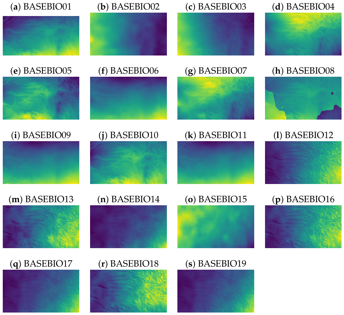
To model the baseline distribution of maize, the 19 standard bioclimatic variables from the CHELSA version 2.1 dataset were used (

Table 2. The 19 standard bioclimatic variables derived from the CHELSA dataset.

Variable Code	Description	Units
BIO1	Annual Mean Temperature	°C
BIO2	Mean Diurnal Range (Mean of monthly (max temp − min temp))	°C
BIO3	Isothermality (BIO2/BIO7) (×100)	%
BIO4	Temperature Seasonality (Standard deviation × 100)	Unitless
BIO5	Max Temperature of Warmest Month	°C
BIO6	Min Temperature of Coldest Month	°C
BIO7	Temperature Annual Range (BIO5–BIO6)	°C
BIO8	Mean Temperature of Wettest Quarter	°C
BIO9	Mean Temperature of Driest Quarter	°C
BIO10	Mean Temperature of Warmest Quarter	°C
BIO11	Mean Temperature of Coldest Quarter	°C
BIO12	Annual Precipitation	mm
BIO13	Precipitation of Wettest Month	mm
BIO14	Precipitation of Driest Month	mm
BIO15	Precipitation Seasonality (Coefficient of Variation)	Unitless
BIO16	Precipitation of Wettest Quarter	mm
BIO17	Precipitation of Driest Quarter	mm
BIO18	Precipitation of Warmest Quarter	mm
BIO19	Precipitation of Coldest Quarter	mm

). These variables are derived from monthly temperature and precipitation data and are designed to be more biologically meaningful for species distribution modeling than simple monthly averages. They represent annual trends (e.g., Annual Mean Temperature), seasonality (e.g., Temperature Seasonality), and limiting environmental factors (e.g., Precipitation of the Driest Quarter), capturing the distinct environmental gradients across the study area (Figure 3).

The CHELSA dataset was specifically chosen over other widely used climatologies, such as WorldClim, due to its more sophisticated downscaling methodology. While WorldClim primarily relies on interpolating data from weather stations, CHELSA employs a more advanced approach that downscales global climate reanalysis data and incorporates orographic predictors, such as wind fields and valley exposition. This results in a more accurate representation of precipitation patterns, particularly in mountainous and topographically complex regions where weather station coverage is often sparse. Given that local and regional topography can significantly influence agricultural conditions, CHELSA’s superior performance in these environments provides a more robust foundation for the model. All bioclimatic data were acquired at a spatial resolution of 30 arc-seconds (∼1 km at the equator), a scale well-suited for regional agricultural analysis. The baseline data represent the 1981–2010 time period. The dataset and its methodology are detailed in [32].

2.5.2. Future Climate Projections

To ensure the robustness of future projections, this study used the multi-model ensemble average from the CHELSA BIOCLIM+ dataset. The data are derived from five distinct Global Climate Models (GCMs) from the Coupled Model Intercomparison Project Phase 6 (CMIP6): GFDL-ESM4, IPSL-CM6A-LR, MPI-ESM1-2-HR, MRI-ESM2-0, and UKESM1-0-LL. By averaging the outputs of these five distinct models across the 19 bioclimatic variables, the resulting projections explicitly account for inter-model variability and structural climate uncertainty, providing a more centralized and robust estimate of future climate conditions than would be possible with any single GCM. This ensemble approach is a standard practice for mitigating the inherent uncertainties of single-model future climate projections [33].

To assess the potential impacts of climate change on maize habitat suitability, future climate projections were also obtained from the CHELSA dataset, which provides downscaled, bias-corrected data from the CMIP6 ensemble. To represent a range of plausible future emission trajectories, two distinct Shared Socioeconomic Pathways (SSPs) were selected:

• SSP3-7.0: A “middle-of-the-road” scenario with moderate emissions.
• SSP5-8.5: A high-challenge, fossil-fuel-intensive development pathway representing a “worst-case” climate future.

For this analysis, two future time periods were selected to represent mid-century and end-of-century climate conditions. These correspond to the 30-year averages for 2041–2070 and 2071–2100. Within the multidimensional CHELSA dataset, these time periods are denoted by their midpoint years. Therefore, bioclimatic variables for 2055 were extracted to represent the 2041–2070 average, and those for 2085 were extracted to represent the 2071–2100 average.

2.5.3. Bioclimate Data Preprocessing

Baseline (1981–2010) and future (2055 and 2085; SSP3-7.0 and SSP5-8.5) bioclimatic variables were extracted from the multidimensional CHELSA datasets [32] via the ArcGIS Pro (v3.5.0) Living Atlas. To ensure spatial alignment with the maize occurrence records prior to modeling, all environmental rasters were clipped to the Kansas boundary, reprojected to the NAD 1983 UTM Zone 14N (EPSG: 26914) coordinate reference system, and resampled from their native 30 arc-second (∼1 km) resolution to the standard 180-m spatial resolution using the bilinear resampling method.

2.5.4. Variable Selection and Dimensionality Reduction

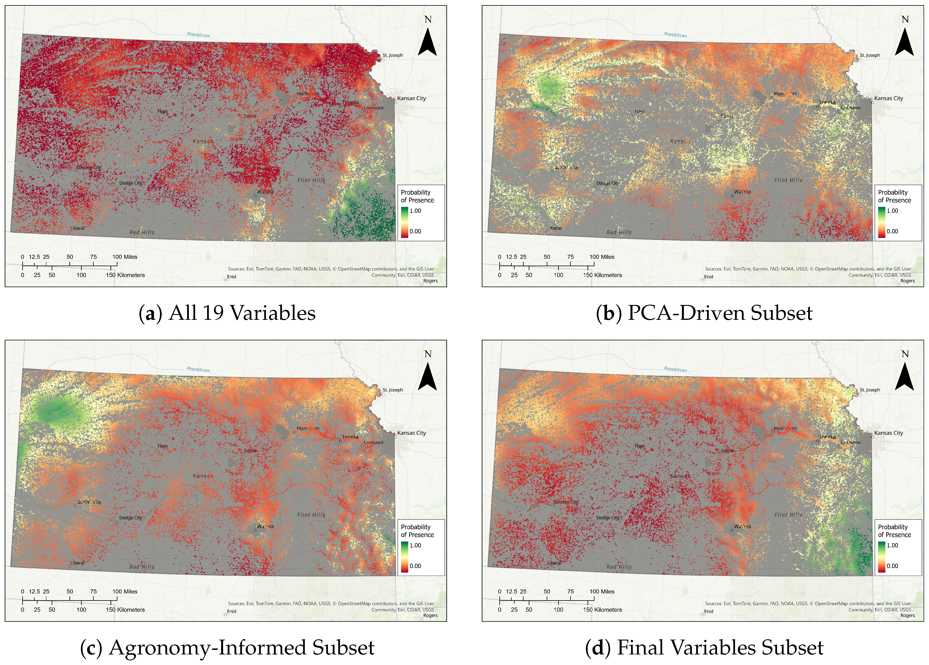
Including the full set of 19 bioclimatic variables into the MaxEnt model introduces severe multicollinearity, as many of these metrics are derived from the same underlying temperature and precipitation data (Figure 4a). Strong collinearity can destabilize model inference, complicate ecological interpretation, and reduce transferability when the correlation structure among predictors changes across time [34,35,36,37]. Furthermore, high-dimensional feature spaces increase the risk of overfitting, in which the algorithm minimizes error by “memorizing” stochastic noise in sampling locations rather than learning the species’ fundamental bioclimatic response surface [38,39]. Although MaxEnt uses regularisation to limit over-complex fits, inappropriate predictor sets and overly complex feature spaces can still overfit the calibration data and degrade performance when projecting to novel conditions [35,40,41].

To identify a robust set of predictors, we employed a hybrid two-stage selection approach that integrated statistical dimensionality reduction with physiological validation. We generated candidate feature sets from both sources to ensure the model captured the primary axes of environmental variation without sacrificing mechanistic realism.

First, we performed an exploratory principal component analysis (PCA) [42] on baseline bioclimate variables to characterize the dominant directions of variance across the study area [38]. We retained the first 5 principal components which together explained ≥95% of the cumulative variance, and identified a PCA-guided candidate subset of original bioclimate variables with the highest absolute loadings across the retained components (BIO4, BIO5, BIO6, BIO12, BIO15). This subset is evaluated in Figure 4b.

Concurrently, we identified an agronomy-informed (literature) subset of original bioclimate predictors (BIO5, BIO10, BIO12, BIO15, BIO18) intended to represent climatic constraints acting during critical maize yield-forming windows (anthesis and grain filling), which are known to be vulnerable to heat and water stress [43,44,45] (Figure 4c).

BIO5 (maximum temperature of the warmest month) represents exposure to extreme mid-summer heat, which is strongly associated with non-linear yield penalties in maize and with reproductive failure via heat impacts on pollen development and fertilization success [45,46]. BIO10 (mean temperature of the warmest quarter) summarises the seasonal thermal regime that governs crop development and phenological pace (thermal-time/degree-day concepts are central in maize agronomy), and it has been shown to yield interpretable suitability optima in continental-scale corn suitability modeling [16,47,48]. Moisture supply during peak demand is represented by BIO18 (precipitation of the warmest quarter), a practical proxy for the reproductive and early grain-fill window in many US maize regions; dryland field evidence identifies a critical summer precipitation period that strongly relates to maize yield outcomes, and MaxEnt response-curve analyses likewise indicate higher suitability with greater warm-quarter precipitation [16,49,50]. Because maize responses depend not only on totals but also on rainfall timing and intermittency, BIO15 (precipitation seasonality; coefficient of variation of monthly precipitation) was included to capture within-year precipitation variability that drives the risk of intra-season dry spells; long-term US analyses show that within-season rainfall/temperature distributions explain yield impacts better than seasonal means alone [16,51]. Finally, BIO12 (annual precipitation) provides a baseline hydroclimatic water-budget context that conditions rainfed yield potential and interacts with atmospheric demand, complementing the season-specific moisture predictors [52,53].

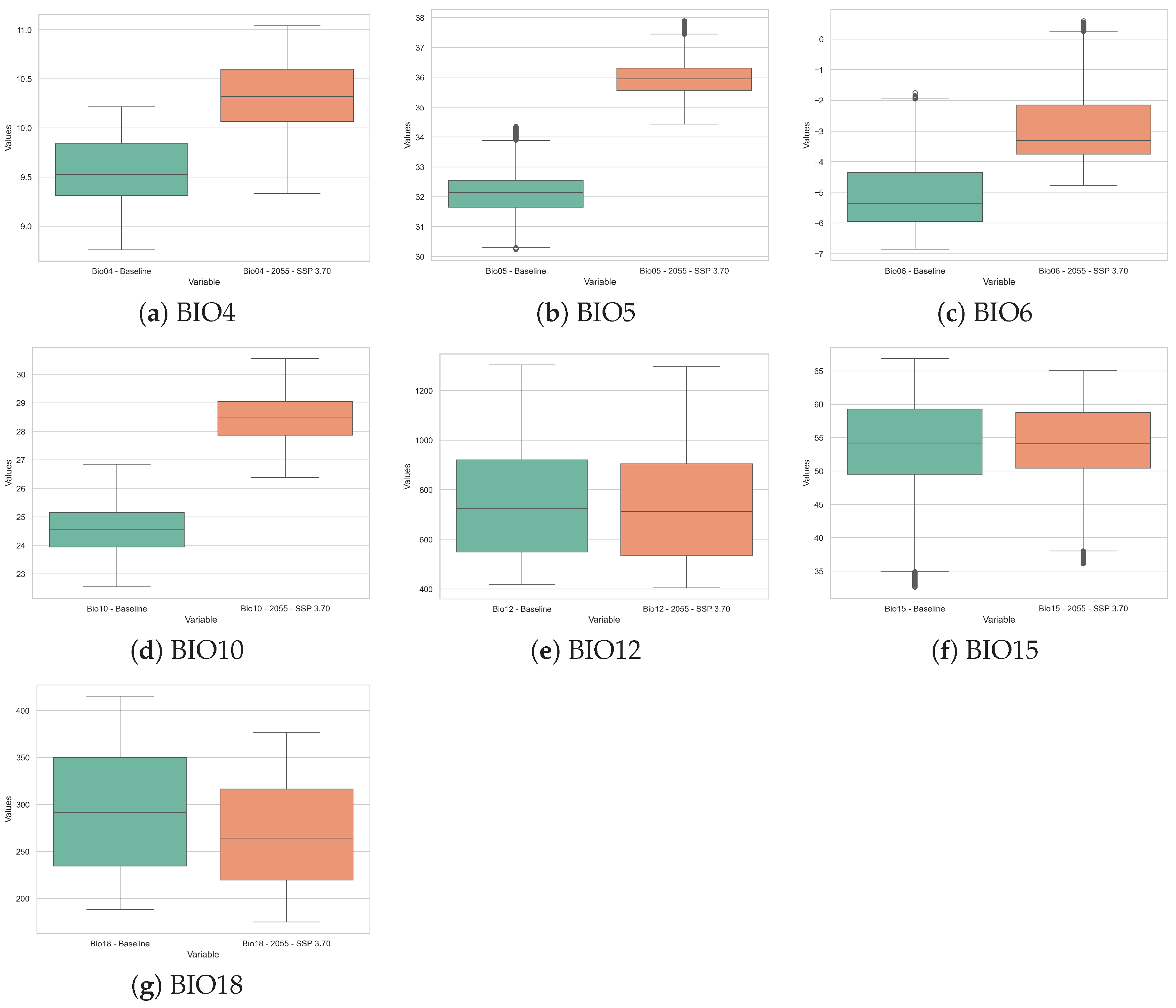
Because SDM projections under climate change can involve univariate range exceedance, we evaluated candidate predictor sets for extrapolation prior to final selection [54,55]. We assessed extrapolation risk under the mid-century projection (2055) for SSP3-7.0. Univariate range shifts for key variables are summarised in Figure 5, which shows strong warming in BIO4, BIO5, and BIO10 relative to the baseline envelope (Figure 5a,b,d). Candidate sets exhibiting extensive strict extrapolation were considered unstable for transfer without explicit clamping/extrapolation controls [54,55,56,57].

This screening showed that predictor sets including warm-season temperature extremes (BIO4, BIO5, and BIO10) exhibited substantial range shifts relative to the baseline training domain (Figure 5a,b,d) and produced materially different 2055 suitability patterns compared with the reduced agronomy subset. Therefore, we excluded volatile warm-season thermal predictors from the final projection set and retained the reduced subset (BIO6, BIO12, BIO15, BIO18) (Figure 4d). This set preserves interpretable moisture-supply and variability constraints (BIO12, BIO15, BIO18) while BIO6 functions primarily as a climatic-gradient proxy within Kansas, rather than as a direct mechanistic descriptor of maize phenology [40,41,58].

2.6. Species Distribution Modeling

2.6.1. Model Setup

Presence Point Generation: The MaxEnt algorithm requires a robust set of occurrence records to characterize the species’ environmental niche. To mitigate sampling bias and ensure the model can discern the specific conditions that favor maize over other agricultural land uses, a stratified random sampling design was employed. Unlike simple random sampling, which may over-represent the most common land-cover types, this approach ensured a balanced distribution of maize occurrences relative to the agricultural background.

The sampling process was implemented in Python (v3.13.5) using the GeoPandas and Rasterio libraries, constrained by a composite exclusion mask. First, the NLCD layer was used to delineate the “plausible agricultural area” by excluding inherently unsuitable categories, such as open water, urban areas, and wetlands (detailed in Section 2.4). Second, this valid area was partitioned into two distinct strata using the binary rainfed maize layer: (1) pixels where maize is present, and (2) background pixels representing agricultural land where maize presence is unknown for the selected CDL year (e.g., other crops or pasture). A calculation example illustrating this pixel-level filtering logic is provided in

Table 3. Pixel classification logic for isolating rainfed maize.

Pixel	M	I	A	R	Interpretation
P1	1	0	1	1	Retained as rainfed maize presence
P2	1	1	1	0	Excluded as irrigated maize (removed from training)
P3	1	0	0	0	Excluded (non-ag domain)
P4	0	0	1	0	Background candidate (agricultural, maize unknown for that year)

Note: Variables: M = CDL maize binary (1: maize, 0: other); I = LANID irrigation binary (1: irrigated, 0: not irrigated); A = agricultural domain mask (1: include, 0: exclude); R = Rainfed maize presence [M × (1 − I) × A].

.

In MaxEnt presence–background modeling, background points represent the environmental conditions available within the study area where maize presence is unknown for the selected year; they are not treated as confirmed absences. ArcGIS Pro (v3.5.0) uses background points to contrast conditions between known presences and the study area to estimate a presence probability surface [59].

Random coordinates were generated iteratively within the Kansas state boundary until a target dataset with the desired number of points was achieved. To optimize this parameter, a sensitivity analysis was conducted using presence-to-background ratios of 50:50, 20:80, 10:90, and 5:95. Based on the stability and realism of the model outputs, a 10:90 ratio was selected. Consequently, the final algorithm drew 10% of the points from the maize-present stratum and 90% from the maize-absent stratum. The resulting dataset was saved as a vector shapefile with a binary attribute indicating the presence (1) and background (0).

Prediction Point Generation: To define the precise locations for future suitability projection, prediction points were derived directly from the binary rainfed maize raster (prepared in Section 2.3). A Python script using the Rasterio library was used to convert this rasterized data to vector format. The algorithm iterated over the grid lattice and, for every pixel identified as maize (value = 1), generated a vector point at the pixel’s centroid. The resulting dataset effectively transforms the continuous raster representation of maize cultivation into a discrete set of coordinate points, which served as the target locations for the MaxEnt model’s predictive queries.

Assembling the Training Dataset: The “presence points” generated serve as the sampling framework for the complete model training dataset. To build the final input file, this point layer was enriched by extracting values from both the species-occurrence raster and all environmental predictor rasters at each point location. This process was executed using Python scripts with the Rasterio and GeoPandas libraries.

First, to classify each of the random points as either an actual maize presence or a background point, the reclassified corn raster (from Section 2.3) was sampled. The script extracted the raster value (1 for corn, 0 for other) at each point’s coordinates and stored this value in a new attribute field.

Next, the corresponding environmental conditions at each point were extracted. The script iterated over all 19 baseline bioclimatic rasters. For each raster, the climate value at each point was sampled and saved to a new field in the attribute table.

The final output was the updated presence points shapefile. Its attribute table contains one row for each presence point, a column indicating whether each point is a presence or background point, and 19 columns detailing the specific baseline environmental conditions at each location. This file provides the complete dataset for training the MaxEnt model.

Assembling the Prediction Dataset: To create the dataset for model projection—that is, to predict suitability across all known maize locations under different climate scenarios, the “prediction points” layer was enriched with the full suite of environmental data.

A Python script iterated over all environmental data layers (baseline and future) and sampled values at each point location, saving them to the point file’s attribute table.

The final prediction points shapefile includes an attribute table in which each row represents a maize occurrence pixel, and the columns contain the full set of environmental predictors for the baseline and future periods. This comprehensive dataset provides the necessary input for projecting the trained model onto current and future climate conditions.

2.6.2. Model Configuration and Parameterization

The suitability modeling was executed using the Presence-only Prediction (MaxEnt) tool within ArcGIS Pro, which implements the maximum entropy algorithm. The model was trained using the “Presence Points” dataset constructed in the previous steps.

To allow for complex, non-linear responses to environmental gradients, the model was configured to utilize a combination of Linear, Quadratic, Product, and Hinge basis expansion functions. This multi-feature approach enables the algorithm to fit a range of ecological response shapes, from simple linear trends to complex thresholds and variable interactions.

Unlike standard species distribution datasets that may require spatial thinning to mitigate observer sampling bias, we did not apply spatial thinning in ArcGIS Pro (Presence-only Prediction: Spatial thinning = NO_THINNING, the default [59]). When thinning is enabled, ArcGIS enforces a minimum nearest-neighbor distance between any two presence points (and between any two background points) via the Minimum Nearest Neighbor Distance parameter; this parameter is not applicable when thinning is not applied. This study retained the full spatial clustering of presence points. In agricultural systems, spatial clustering is not an artifact of sampling effort but an inherent characteristic of the landscape, driven by the contiguous nature of soil types, field boundaries, and land management units. Enforcing spatial independence in this context would artificially fragment the crop’s realized niche, potentially removing valid data points that represent the core of the high-suitability envelope.

To assess model performance and robustness, a 10-fold random cross-validation scheme was employed using the native capabilities of the ArcGIS Pro Presence-only Prediction tool. We acknowledge that random k-fold cross-validation can be susceptible to spatial data leakage in highly contiguous datasets, potentially inflating internal performance metrics due to spatial autocorrelation. However, spatial blocking was not enforced because the contiguous clustering of agricultural fields in this study reflects genuine biophysical landscape reality rather than observer sampling bias, as described previously. Furthermore, to mitigate the limitations of internal random cross-validation and verify true predictive reliability, model outputs were subjected to a robust independent external validation against 30 years of historical USDA county-level production records (Section 3.2). The occurrence data were randomly partitioned into 10 folds; in each iteration, the model was trained on 90% of the data and tested on the remaining 10%, providing a robust estimate of predictive accuracy and preventing overfitting.

Beyond the specified basis expansion functions, all other MaxEnt hyperparameters, including the regularization multiplier, were retained at their ArcGIS Pro defaults. Systematic manual tuning of regularization parameters was not conducted because our variable selection and dimensionality reduction process (detailed in Section 2.5.4) effectively constrained the predictor space. By using a subset of variables, we inherently reduced the model’s dimensionality, thereby mitigating the primary risk of overfitting the training data prior to algorithmic calibration.

The model output was generated as probability of presence (PoP; 0–1) using the Complementary Log-Log (ClogLog) link function. This transformation scales the raw MaxEnt output into a continuous probability estimate ranging from 0 to 1, representing the bioclimatic suitability for rainfed maize presence, conditional on the modeling domain and predictors. In this study, PoP is not a yield forecast and does not explicitly encode management, soils, or cultivar selection. Because projected climatic suitability does not account for genetic and management adaptations (such as drought-tolerant hybrids or adjusted fertility management), the resulting probabilities should be interpreted as scenario-based climatic pressures rather than deterministic yield losses.

Finally, the optimized model was projected onto the future climate scenarios. This was achieved by mapping the explanatory variables of the trained model (Baseline Bioclimates) to their corresponding counterparts in the future datasets (e.g., matching BaseBio01 to Bio01_55_3 for the mid-century SSP3-7.0 scenario). This projection process was repeated for all combinations of time periods (2055, 2085) and emission pathways (SSP3-7.0, SSP5-8.5) to generate the final suitability maps.

3. Results and Discussion

3.1. Model Performance

To assess the predictive performance and robustness of the MaxEnt model, we utilized a combination of statistical metrics and biological plausibility checks. First, we examined the Receiver Operating Characteristic (ROC) curve, a standard metric for evaluating the quality of presence-only models [16]. Accordingly, threshold-dependent metrics, such as Cohen’s Kappa, were excluded because MaxEnt generates continuous probability outputs from presence-background data rather than definitive presence-absence classifications. An ideal ROC curve follows an “L-shape”, rising rapidly along the y-axis, which maximizes the Area Under the Curve (AUC). The AUC value serves as the primary indicator of model accuracy, ranging from $0.0$ to $1.0$, with values closer to $1.0$ indicating a high-quality model that effectively discriminates between suitable and unsuitable habitats.

3.1.1. ROC

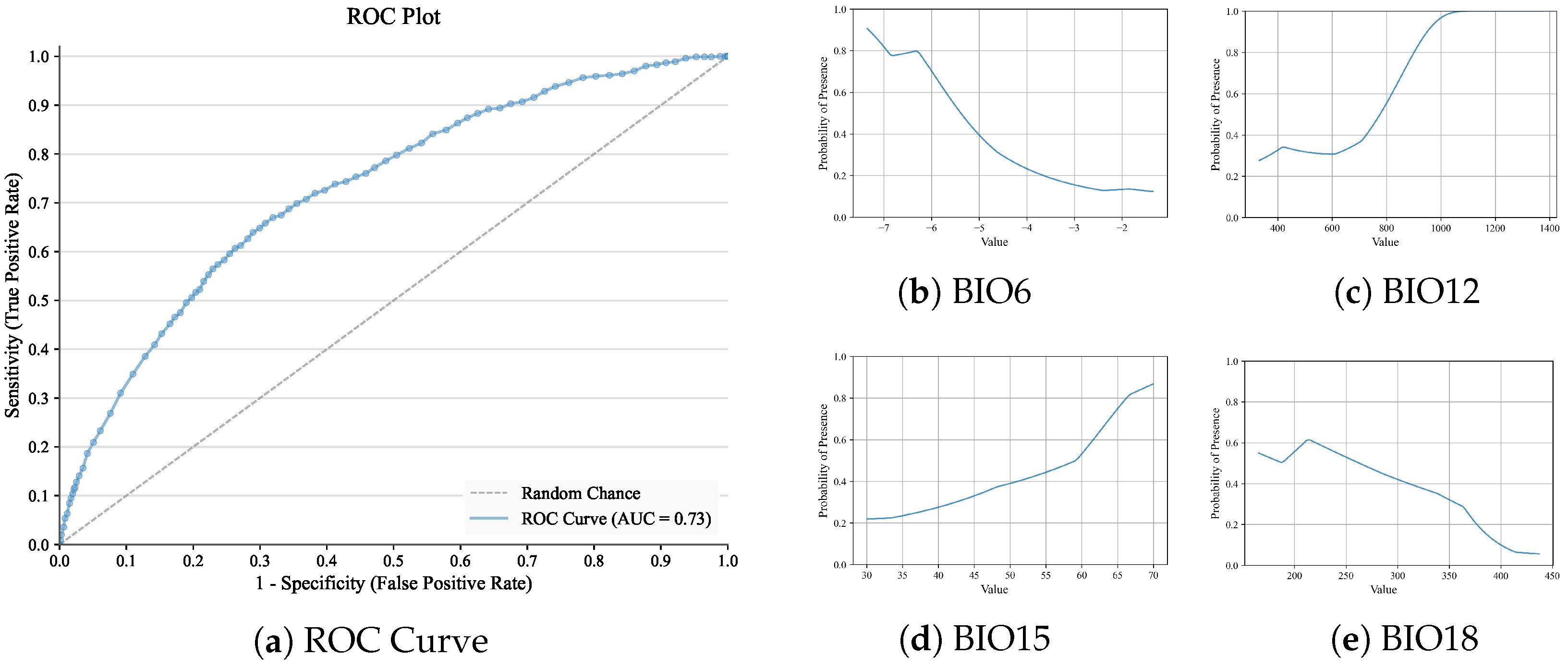
Model performance was assessed using the Receiver Operating Characteristic (ROC) curve, shown in Figure 6a. The ROC curve summarizes the trade-off between sensitivity (true positive rate) and specificity (false positive rate) across a range of probability thresholds.

The curve rises above the 1:1 diagonal, indicating predictive skill beyond random expectation. A relatively smooth progression reflects stable classification behavior across probability thresholds. Sensitivity increases gradually as specificity decreases, suggesting that the model is moderately conservative in classifying presence. With an AUC value of 0.73, the curve’s general shape suggests a mid-to-high performance range typical of ecological niche models built from presence-only data.

Uncertainty is inherent in presence-only frameworks, as background points can include a mixture of suitable and unsuitable environments, and the MaxEnt model assumes that sampling bias is minimized. These limitations are acknowledged when interpreting the ROC curve and incorporated into the overall assessment of model skill.

3.1.2. Response Curves

The partial response curves (Figure 6b–e) provide physiological insight into the specific environmental thresholds governing the realized niche of rainfed maize in Kansas. Among the selected predictors, Annual Precipitation (BIO12) exhibits the most distinct constraint on distribution (Figure 6c). The response follows a sigmoidal logistic function, revealing a critical hydrological threshold. Probability of presence remains low (<0.4) in regions receiving less than 700 mm of annual rainfall, reflecting the high risk of crop failure in the semi-arid western steppe without irrigation. Suitability increases rapidly between 700 mm and 900 mm, plateauing near 1.0 at approximately 1000 mm, effectively demarcating the transition from marginal to optimal rainfed zones.

Min Temperature of Coldest Month (BIO06) displays a negative relationship (Figure 6b), where suitability is highest at lower winter minimums (≈−7 °C). In the context of Kansas, this variable likely serves as a latitudinal proxy, favoring the state’s northern tier, which aligns with the extension of the Corn Belt, distinct from the warmer southern counties, where evapotranspiration demands may be higher.

The influence of temporal water availability is further clarified by Precipitation Seasonality (BIO15) and Precipitation of Warmest Quarter (BIO18). The positive slope of BIO15 (Figure 6d) indicates a preference for high seasonality, characteristic of the continental climate where precipitation is concentrated in the growing season rather than distributed uniformly. However, BIO18 (Figure 6e) reveals a non-linear optimization; while moderate summer rainfall is essential, suitability peaks at approximately 220 mm and declines sharply beyond 350 mm. This upper limit likely reflects a combination of environmental factors, including the exclusion of the high-rainfall Flint Hills region (predominantly pastureland) and the potential for excess moisture stress or disease pressure in the humid subtropical Southeast.

3.2. Model Validation

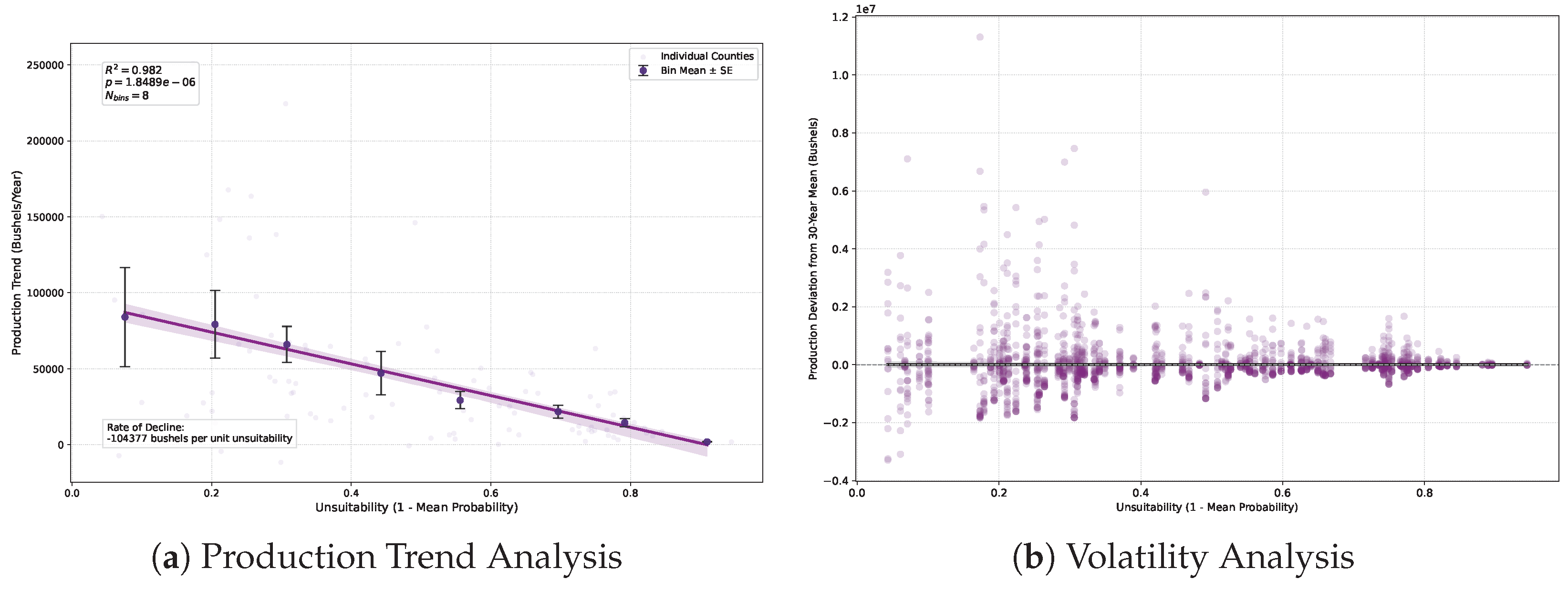
Beyond standard statistical metrics, we validated the model’s biological and economic relevance by cross-referencing the derived Suitability Index with 30 years of independent USDA production data (1981–2010) [60]. First, to evaluate long-term viability, we computed the linear production trend (slope in Bushels/year) for each county and regressed these trends against the county’s ’Unsuitability’ (defined as $1-\mathrm{Mean}\mathrm{Probability}\mathrm{of}\mathrm{Presence}$), using binned aggregation to mitigate stochastic noise. Second, to assess production stability, we performed a volatility analysis by calculating annual production anomalies, defined as the deviation of each year’s harvest from the county’s 30-year mean. These anomalies were plotted against unsuitability to characterize the relationship between habitat quality and yield variance (heteroscedasticity) across the study region depicted in Figure 7.

The production-trend analysis reveals a strong negative relationship between modeled unsuitability and long-term production performance (Figure 7a). Although individual counties exhibit local scatter, the binned means decline almost linearly with increasing unsuitability, corresponding to an estimated decline of 104,377 bushels/year for each unit increase in unsuitability. In practical terms, counties classified by the model as more climatically suitable have historically maintained stronger positive production trends, whereas counties with higher unsuitability show substantially weaker long-term gains. This close agreement between the suitability gradient and an independent historical production record supports the agricultural relevance of the MaxEnt predictions and indicates that the model is capturing meaningful bioclimatic constraints rather than a purely statistical spatial pattern.

The volatility analysis provides complementary but more nuanced validation (Figure 7b). Rather than showing a strong directional shift in anomaly sign across the unsuitability gradient, the dominant pattern is a clear change in the spread of the anomalies. Counties with low to moderate unsuitability exhibit the widest range of annual departures from their 30-year mean, while highly unsuitable counties cluster near comparatively small deviations.

Because these anomalies are expressed in absolute bushels, this pattern is best interpreted as reflecting differences in production capacity rather than intrinsic climatic stability alone. Moreover, county production totals can include irrigated contributions, whereas the MaxEnt model is calibrated to rainfed presence. Irrigation in western/central Kansas is closely linked to High Plains aquifer withdrawals that can buffer climatic limitations [29]. Favorable counties support larger harvests and therefore larger absolute year-to-year swings, whereas marginal counties are constrained to persistently lower production levels. Taken together, these two analyses show that the suitability index captures both long-term productive capacity and the upper envelope of county-level maize production across Kansas.

3.3. Baseline Model Evaluation and Variable Selection

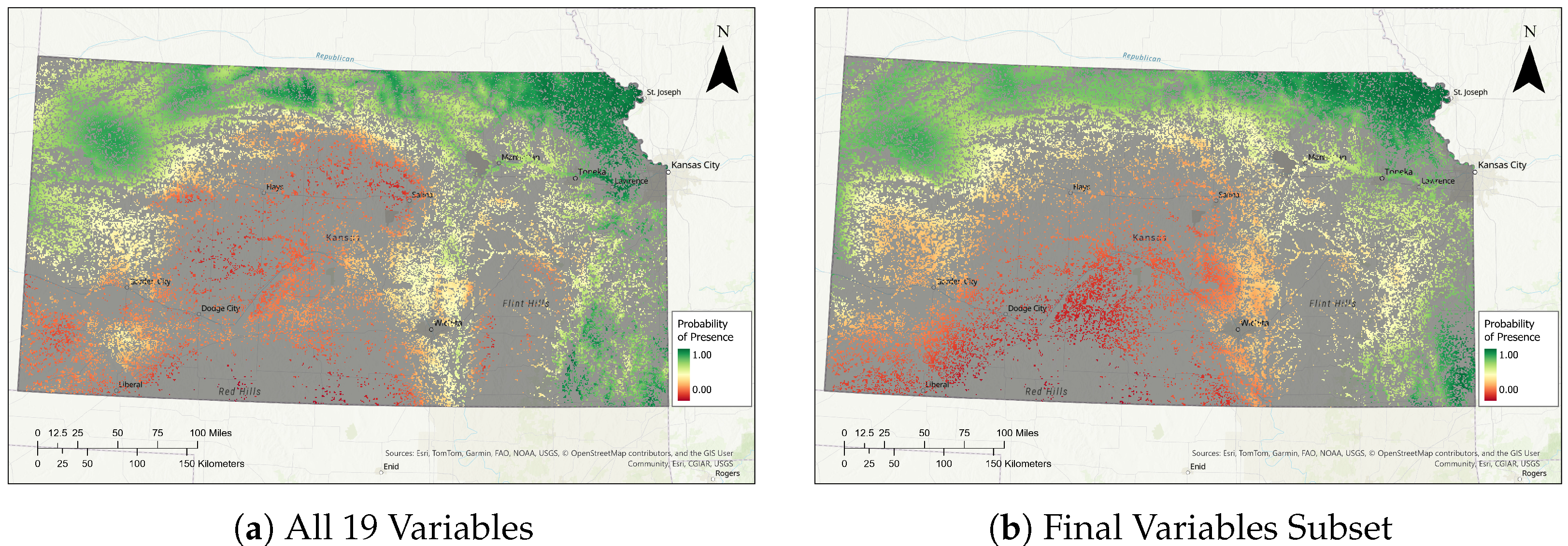
The immediate output of the MaxEnt projection is a vector point layer representing the prediction dataset, with the calculated Probability of Presence (POP) stored as a column in the attribute table. To translate these discrete point predictions into a continuous spatial representation of habitat suitability, we used the Point to Raster tool in ArcGIS Pro. This process converted the point features into a raster surface, resulting in a final map with continuous pixel values ranging from 0 (unsuitable) to 1 (highly suitable) (Figure 8).

To validate the parsimonious “Agronomy Subset” (BIO06, BIO12, BIO15, BIO18) (Figure 8a), its baseline predictions were spatially cross-referenced against a “full” model trained on all 19 bioclimatic variables (Figure 8b).

The comparison reveals a high degree of spatial concordance between the two models. Both outputs successfully capture the primary longitudinal gradient of suitability, identifying the humid eastern counties and the northern tier as highly suitable (green), while correctly classifying the semi-arid southwestern region as marginal or unsuitable (red/orange). Notably, the optimized 4-variable model preserves the nuanced localized patterns, such as the distinct pocket of suitability in the high-elevation northwestern counties, without relying on the full high-dimensional feature space.

The similarity between these surfaces confirms that the selected subset of four variables effectively encapsulates the dominant environmental drivers of rainfed maize distribution in Kansas. By reproducing the complex baseline with fewer parameters, the Agronomy Subset minimizes the risk of overfitting and multicollinearity, justifying its use for the robust future projections presented in subsequent sections.

3.4. Future Projections and Habitat Contraction

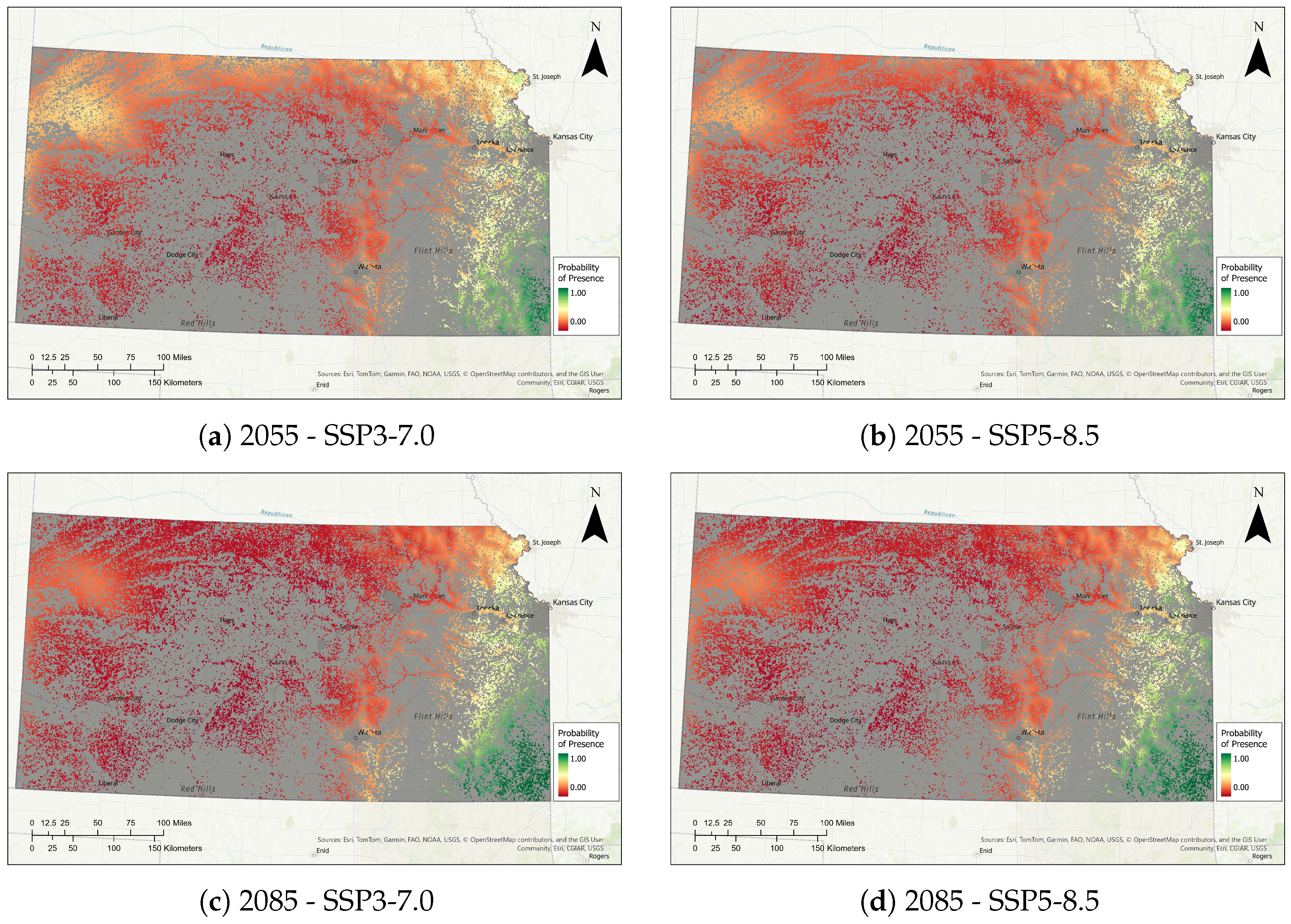
The projected suitability surfaces for the mid- and end-of-century periods reveal a progressive and severe contraction of the realized niche for rainfed maize in Kansas (Figure 9). Under all modeled scenarios, the primary trend is a longitudinal eastward migration of the cultivation boundary, driven by the intensifying decoupling of thermal suitability and precipitation availability.

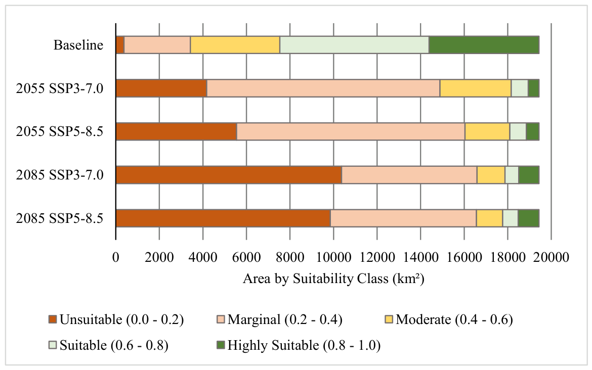
To explicitly quantify the spatial contraction of the realized niche, the projected area for each suitability class was extracted and calculated across all time periods and emission pathways (

Table 4. Projected spatial extent (${\mathrm{km}}^2$) of climatic suitability classes for rainfed maize across baseline (1981–2010) and future scenarios. Values represent the absolute area within the defined agricultural modeling domain.

Suitability	Baseline	2055	2055	2085	2085
Class (PoP)	(1981–2010)	(SSP3-7.0)	(SSP5-8.5)	(SSP3-7.0)	(SSP5-8.5)
0.0–0.2	373	4172	5543	10,370	9854
0.2–0.4	3053	10,716	10,492	6217	6708
0.4–0.6	4111	3268	2059	1289	1206
0.6–0.8	6849	785	760	629	711
0.8–1.0	5050	495	582	931	957

, Figure 10). Under baseline conditions (1981–2010), the Kansas agricultural landscape is predominantly characterized by favorable climatic conditions for rainfed maize; over 60% of the modeled domain (11,899 ${\mathrm{km}}^2$) is classified as ‘Suitable’ or ‘Highly Suitable’, while strictly ‘Unsuitable’ conditions are confined to a marginal 373 ${\mathrm{km}}^2$.

However, the future projections reveal a severe, progressive collapse of this optimal habitat. By mid-century (2055), the area deemed ’Highly Suitable’ experiences an abrupt decline of approximately 90%, plummeting from 5050 ${\mathrm{km}}^2$ to just under 600 ${\mathrm{km}}^2$ across both SSP scenarios. Concurrently, the ‘Unsuitable’ geographic footprint expands by more than an order of magnitude, encroaching upon 5543 ${\mathrm{km}}^2$ under the higher-emission SSP5-8.5 pathway.

This climatic squeeze intensifies drastically by the end of the century (2085). As visualized in Figure 10, the optimal and moderate suitability classes are almost entirely consumed by marginal or hostile environmental thresholds. By 2085, regardless of the emission trajectory, roughly 50% of the historically viable rainfed maize domain (approximately 10,000 ${\mathrm{km}}^2$) becomes fundamentally unsuited for cultivation. This quantitative shift underscores the severe longitudinal migration of the climatic boundary, indicating that without supplemental irrigation, only the easternmost edge of the state will retain the hydro-thermal balance required to sustain reliable production.

3.4.1. Mid-Century Shifts (2055)

By 2055, the divergence from baseline conditions is already stark. Under the SSP3-7.0 scenario (Figure 9a), the western third of the state—historically a semi-arid production zone—transitions to near-zero probability of presence (indicated in red). This region effectively falls below the critical hydrological thresholds defined by the model’s precipitation variables (BIO12 and BIO18).

The higher-emission SSP5-8.5 scenario for the same period (Figure 9b) accelerates this trend. While the spatial extent of the “unsuitable” western zone remains broadly similar to that in SSP3-7.0, the central transition zone exhibits greater fragmentation. The “buffer” region of moderate suitability (yellow/orange) thins perceptibly, suggesting that the velocity of climate change in the high-emissions pathway is already eroding the resilience of the central counties by mid-century.

3.4.2. End-of-Century Intensification (2085)

The distinction between scenarios and the severity of habitat loss becomes most pronounced by 2085. The progression from 2055 to 2085 illustrates a collapse of the central transition zone. Under SSP3-7.0 (Figure 9c), the area of unsuitability expands significantly eastward, encroaching into the central agricultural belt.

However, the most extreme contraction is observed under the SSP5-8.5 scenario for 2085 (Figure 9d). In this “worst-case” projection, the model indicates that nearly two-thirds of the state becomes climatically unsuitable for rainfed maize. The suitable habitat (green) is effectively restricted to the easternmost tier of counties, where moisture regimes remain sufficient to buffer against extreme thermal stress. This projection implies that, without significant agronomic adaptation or widespread irrigation expansion, the geographic center of Kansas maize production would shift entirely to the humid eastern border.

4. Conclusions

This study successfully established a high-resolution, probabilistic model of rainfed maize suitability across Kansas’s climatic transition zone using a Maximum Entropy (MaxEnt) approach. By integrating a novel data-filtering workflow that combined the USDA Cropland Data Layers with LANID irrigation masks, we were able to isolate strictly rainfed occurrences. This methodological refinement addressed a critical gap in regional agricultural modeling, ensuring that the resulting projections reflect true bioclimatic limitations rather than the confounding influence of aquifer-supported irrigation. Although numeric PoP values and mapped extents are Kansas-specific, the workflow is transferable to other regions with comparable crop-type maps, irrigation-extent products, and downscaled climate predictors. Key transferable steps include (i) delineating a meaningful study area and background sample, (ii) masking irrigation to isolate rainfed climatic constraints (LANID), (iii) using consistent downscaled climate datasets (CHELSA), and (iv) implementing structured validation appropriate to spatial data. Following MaxEnt best-practice guidance, transfer applications should re-evaluate background sampling, predictor choice, and validation design, because MaxEnt outputs depend on user decisions about inputs and settings [35,61].

The model, with an AUC of 0.73 and robust external validation against long-term county-level production records, reveals that the optimal cultivation niche for rainfed maize is highly sensitive to projected climatic shifts in the 21st century. Under both SSP3-7.0 and SSP5-8.5 scenarios, our projections indicate a distinct eastward contraction of suitable habitats, with highly suitable areas plummeting by approximately 90% by mid-century, and roughly half of the historically viable domain becoming fundamentally unsuited by 2085. Western and Central Kansas, regions historically dependent on the interplay between precipitation and supplemental irrigation, are projected to experience a significant decline in climatic suitability due to rising thermal stress and increased precipitation variability.

These findings have profound implications for regional water policy and agricultural sustainability. The predicted contraction of rainfed suitability suggests that the pressure on the High Plains Aquifer may intensify as producers attempt to buffer against climatic deficits, potentially accelerating groundwater depletion. Consequently, the “transition zone” of arable land is effectively migrating eastward, necessitating a re-evaluation of long-term cropping strategies in the Great Plains.

While this study provides a robust bioclimatic baseline, it assumes a static realized climatic tolerance space. Therefore, our projected suitability contractions should be interpreted as mounting climatic pressures rather than definitive agricultural failures, as they do not account for future human adaptation. Future research should aim to integrate these bioclimatic projections with mechanistic crop growth models to account for potential adaptation strategies, such as the introduction of heat-tolerant hybrids or shifts in planting dates. Additionally, incorporating socio-economic variables could further refine predictions by capturing the human dimensions of land-use change in response to these evolving climatic constraints.

References

1. Kogo, B.K.; Kumar, L.; Koech, R.; Kariyawasam, C.S. Modelling Climate Suitability for Rainfed Maize Cultivation in Kenya Using a Maximum Entropy (MaxENT) Approach. Agronomy 2019, 9, 727. [Google Scholar] [CrossRef]
2. Tang, X.; Liu, H. Climate suitability for summer maize on the North China Plain under current and future climate scenarios. Int. J. Climatol. 2021, 41, E2644–E2661. [Google Scholar] [CrossRef]
3. Ojara, M.A.; Yunsheng, L.; Ongoma, V.; Mumo, L.; Akodi, D.; Ayugi, B.; Ogwang, B.A. Projected changes in East African climate and its impacts on climatic suitability of maize production areas by the mid-twenty-first century. Environ. Monit. Assess. 2021, 193, 831. [Google Scholar] [CrossRef]
4. Gao, Y.; Zhang, A.; Yue, Y.; Wang, J.; Su, P. Predicting Shifts in Land Suitability for Maize Cultivation Worldwide Due to Climate Change: A Modeling Approach. Land 2021, 10, 295. [Google Scholar] [CrossRef]
5. Estrada-Contreras, I.; Pavón, N.P.; Cadena, J.B.; Bourg, A. Ecological niche models of productive corn races under climate change scenarios in central-eastern Mexico. Agron. J. 2023, 115, 1023–1036. [Google Scholar] [CrossRef]
6. Chemura, A.; Schauberger, B.; Gornott, C. Impacts of climate change on agro-climatic suitability of major food crops in Ghana. PLoS ONE 2020, 15, e0229881. [Google Scholar] [CrossRef]
7. Monterroso Rivas, A.; Conde Álvarez, C.; Rosales Dorantes, G.; Gómez Díaz, J.D.; Gay García, C. Assessing current and potential rainfed maize suitability under climate change scenarios in México. Atmósfera 2011, 24, 53–67. [Google Scholar]
8. Yu, J.L.; Qi, H.; Nie, L.X.; Zhang, W.J.; Zheng, H.B.; Liu, M.; Lin, Z.Q.; Gao, M.C. Effects of Environment Variables on Maize Yield and Ear Characters. Adv. Mater. Res. 2013, 726–731, 106–113. [Google Scholar] [CrossRef]
9. Abendroth, L.J.; Miguez, F.E.; Castellano, M.J.; Carter, P.R.; Messina, C.D.; Dixon, P.M.; Hatfield, J.L. Lengthening of maize maturity time is not a widespread climate change adaptation strategy in the US Midwest. Glob. Change Biol. 2021, 27, 2426–2440. [Google Scholar] [CrossRef]
10. Chen, X.; Shi, Z.; Xiao, D.; Lu, Y.; Bai, H.; Zhang, M.; Ren, D.; Qi, Y.; Song, S. Assessment of extreme climate stress across China’s maize harvest region in CMIP6 simulations. Front. Environ. Sci. 2024, 12, 1503141. [Google Scholar] [CrossRef]
11. L Hoffman, A.; R Kemanian, A.; E Forest, C. The response of maize, sorghum, and soybean yield to growing-phase climate revealed with machine learning. Environ. Res. Lett. 2020, 15, 094013. [Google Scholar] [CrossRef]
12. Portalanza, D.; Pántano, V.C.; Zuluaga, C.F.; Benso, M.R.; Corrales Suastegui, A.; Castillo, N.; Solman, S. Can extreme climatic and bioclimatic indices reproduce soy and maize yields in Latin America? Part 1: An observational and modeling perspective. Environ. Earth Sci. 2024, 83, 175. [Google Scholar] [CrossRef]
13. Torabi, F.; Monavarian, A.; Nooraei Beidokhti, A.; Sharda, V.; Moore, T. Effects of Wood Anatomy, Climate, Soil Type, and Plant Configuration Variables on Urban Tree Transpiration in the Context of Urban Runoff Reduction: A Systematic Metadata Analysis. Sustainability 2026, 18, 4157. [Google Scholar] [CrossRef]
14. Ali, S.; Umair, M.; Makanda, T.A.; Shi, S.; Hussain, S.A.; Ni, J. Modeling Current and Future Potential Land Distribution Dynamics of Wheat, Rice, and Maize under Climate Change Scenarios Using MaxEnt. Land 2024, 13, 1156. [Google Scholar] [CrossRef]
15. Estes, L.D.; Bradley, B.A.; Beukes, H.; Hole, D.G.; Lau, M.; Oppenheimer, M.G.; Schulze, R.; Tadross, M.A.; Turner, W.R. Comparing mechanistic and empirical model projections of crop suitability and productivity: Implications for ecological forecasting. Glob. Ecol. Biogeogr. 2013, 22, 1007–1018. [Google Scholar] [CrossRef]
16. Fitzgibbon, A.; Pisut, D.; Fleisher, D. Evaluation of Maximum Entropy (Maxent) Machine Learning Model to Assess Relationships between Climate and Corn Suitability. Land 2022, 11, 1382. [Google Scholar] [CrossRef]
17. Ali, S.; Makanda, T.A.; Umair, M.; Ni, J. MaxEnt model strategies to studying current and future potential land suitability dynamics of wheat, soybean and rice cultivation under climatic change scenarios in East Asia. PLoS ONE 2023, 18, e0296182. [Google Scholar] [CrossRef]
18. Warton, D.I.; Renner, I.W.; Ramp, D. Model-Based Control of Observer Bias for the Analysis of Presence-Only Data in Ecology. PLoS ONE 2013, 8, e79168. [Google Scholar] [CrossRef] [PubMed]
19. Chemura, A.; Nangombe, S.S.; Gleixner, S.; Chinyoka, S.; Gornott, C. Changes in Climate Extremes and Their Effect on Maize (Zea mays L.) Suitability Over Southern Africa. Front. Clim. 2022, 4, 890210. [Google Scholar] [CrossRef]
20. Aber, J.S. (Ed.) Physical Geography of Kansas; Educational Series 19; Kansas Geological Survey: Lawrence, KS, USA, 2020. [Google Scholar]
21. National Oceanic and Atmospheric Administration (NOAA); National Centers for Environmental Information (NCEI). Kansas State Climate Summary; NOAA Technical Report NESDIS 150-KS; NOAA: Asheville, NC, USA, 2022.
22. Kansas Office of the State Climatologist. Kansas Climate Basics. Available online: https://mesonet.k-state.edu/climate/basics/ (accessed on 11 April 2026).
23. Lin, X.; Harrington, J.A., Jr.; Ciampitti, I.; Gowda, P.; Brown, D.; Kisekka, I. Kansas Trends and Changes in Temperature, Precipitation, Drought, and Frost-Free Days from the 1890s to 2015. J. Contemp. Water Res. Educ. 2017, 162, 18–30. [Google Scholar] [CrossRef]
24. Peel, M.C.; Finlayson, B.L.; McMahon, T.A. Updated world map of the Köppen-Geiger climate classification. Hydrol. Earth Syst. Sci. 2007, 11, 1633–1644. [Google Scholar] [CrossRef]
25. United States Department of Agriculture, National Agricultural Statistics Service. Crop Production 2024 Summary; Technical Report; United States Department of Agriculture: Washington, DC, USA, 2025.
26. Sen, R.; Sharda, V.; Zambreski, Z.T.; Onyekwelu, I.; Nelson, K.S. Effects of future climate on suitability of major crops in Eastern Kansas River Basin. J. Water Land Dev. 2024, 145–157. [Google Scholar] [CrossRef]
27. U.S. Census Bureau. TIGER/Line Shapefile, 2023, State, Kansas, Current State Boundaries. Shapefile. 2023. Available online: https://www.census.gov/geographies/mapping-files/time-series/geo/tiger-line-file.html (accessed on 5 November 2025).
28. United States Department of Agriculture, National Agricultural Statistics Service. Cropland Data Layer. 2024. Available online: https://croplandcros.scinet.usda.gov/ (accessed on 8 October 2025).
29. Buchanan, R.C.; Wilson, B.B.; James J. Butler, J. The High Plains Aquifer; Public Information Circular 18; Kansas Geological Survey: 2023, Revised January 2023. Available online: https://kgs.ku.edu/high-plains-aquifer (accessed on 5 February 2026).
30. Xie, Y.; Lark, T.J.; Brown, J.F.; Gibbs, H.K. Annual maps of irrigated cropland in the conterminous United States, 1997–2017. Earth Syst. Sci. Data 2021, 13, 5689–5710. [Google Scholar] [CrossRef]
31. U.S. Geological Survey; MRLC Consortium. National Land Cover Database (NLCD) 2021: Land Cover (CONUS). Raster dataset. 2021. Available online: https://www.mrlc.gov/data (accessed on 5 November 2025).
32. Karger, D.N.; Conrad, O.; Böhner, J.; Kawohl, T.; Kreft, H.; Soria-Auza, R.W.; Zimmermann, N.E.; Linder, H.P.; Kessler, M. Climatologies at high resolution for the earth’s land surface areas. Sci. Data 2017, 4, 170122. [Google Scholar] [CrossRef] [PubMed]
33. Brun, P.; Zimmermann, N.E.; Hari, C.; Pellissier, L.; Karger, D.N. Global climate-related predictors at kilometer resolution for the past and future. Earth Syst. Sci. Data 2022, 14, 5573–5603. [Google Scholar] [CrossRef]
34. Dormann, C.F.; Elith, J.; Bacher, S.; Buchmann, C.; Carl, G.; Carré, G.; Marquéz, J.R.G.; Gruber, B.; Lafourcade, B.; Leitão, P.J.; et al. Collinearity: A review of methods to deal with it and a simulation study evaluating their performance. Ecography 2012, 36, 27–46. [Google Scholar] [CrossRef]
35. Merow, C.; Smith, M.J.; Silander, A.J., Jr. A practical guide to MaxEnt for modeling species’ distributions: What it does, and why inputs and settings matter. Ecography 2013, 36, 1058–1069. [Google Scholar] [CrossRef]
36. De Marco, P.; Nóbrega, C.C. Evaluating collinearity effects on species distribution models: An approach based on virtual species simulation. PLoS ONE 2018, 13, e0202403. [Google Scholar] [CrossRef]
37. Feng, X.; Park, D.S.; Liang, Y.; Pandey, R.; Papeş, M. Collinearity in ecological niche modeling: Confusions and challenges. Ecol. Evol. 2019, 9, 10365–10376. [Google Scholar] [CrossRef]
38. Li, Y.; Li, M.; Li, C.; Liu, Z. Optimized Maxent Model Predictions of Climate Change Impacts on the Suitable Distribution of Cunninghamia lanceolata in China. Forests 2020, 11, 302. [Google Scholar] [CrossRef]
39. Morales, N.S.; Fernández, I.C.; Baca-González, V. MaxEnt’s parameter configuration and small samples: Are we paying attention to recommendations? A systematic review. PeerJ 2017, 5, e3093. [Google Scholar] [CrossRef] [PubMed]
40. Warren, D.L.; Seifert, S.N. Ecological niche modeling in Maxent: The importance of model complexity and the performance of model selection criteria. Ecol. Appl. 2011, 21, 335–342. [Google Scholar] [CrossRef] [PubMed]
41. Radosavljevic, A.; Anderson, R.P. Making better Maxent models of species distributions: Complexity, overfitting and evaluation. J. Biogeogr. 2013, 41, 629–643. [Google Scholar] [CrossRef]
42. Jolliffe, I.T.; Cadima, J. Principal component analysis: A review and recent developments. Philos. Trans. R. Soc. A Math. Phys. Eng. Sci. 2016, 374, 20150202. [Google Scholar] [CrossRef]
43. BarnabÁS, B.; Jäger, K.; Fehér, A. The effect of drought and heat stress on reproductive processes in cereals. Plant Cell Environ. 2007, 31, 11–38. [Google Scholar] [CrossRef]
44. Badu-Apraku, B.; Hunter, R.B.; Tollenaar, M. Effect of Temperature During Grain Filling on Whole Plant and Grain Yield in Maize (Zea mays L.). Can. J. Plant Sci. 1983, 63, 357–363. [Google Scholar] [CrossRef]
45. Schlenker, W.; Roberts, M.J. Nonlinear temperature effects indicate severe damages to U.S. crop yields under climate change. Proc. Natl. Acad. Sci. USA 2009, 106, 15594–15598. [Google Scholar] [CrossRef]
46. Begcy, K.; Nosenko, T.; Zhou, L.Z.; Fragner, L.; Weckwerth, W.; Dresselhaus, T. Male Sterility in Maize after Transient Heat Stress during the Tetrad Stage of Pollen Development. Plant Physiol. 2019, 181, 683–700. [Google Scholar] [CrossRef]
47. Gilmore, E.C., Jr.; Rogers, J.S. Heat Units as a Method of Measuring Maturity in Corn1. Agron. J. 1958, 50, 611–615. [Google Scholar] [CrossRef]
48. McMaster, G. Growing degree-days: One equation, two interpretations. Agric. For. Meteorol. 1997, 87, 291–300. [Google Scholar] [CrossRef]
49. Nielsen, D.C.; Halvorson, A.D.; Vigil, M.F. Critical precipitation period for dryland maize production. Field Crops Res. 2010, 118, 259–263. [Google Scholar] [CrossRef]
50. Huang, C.; Duiker, S.; Deng, L.; Fang, C.; Zeng, W. Influence of Precipitation on Maize Yield in the Eastern United States. Sustainability 2015, 7, 5996–6010. [Google Scholar] [CrossRef]
51. Hu, Q.; Buyanovsky, G. Climate Effects on Corn Yield in Missouri. J. Appl. Meteorol. 2003, 42, 1626–1635. [Google Scholar] [CrossRef]
52. Luan, X.; Bommarco, R.; Vico, G. Coordinated evaporative demand and precipitation maximize rainfed maize and soybean crop yields in the USA. Ecohydrology 2022, 16, e2500. [Google Scholar] [CrossRef]
53. Haarhoff, S.J.; Swanepoel, P.A. Plant Population and Maize Grain Yield: A Global Systematic Review of Rainfed Trials. Crop Sci. 2018, 58, 1819–1829. [Google Scholar] [CrossRef]
54. Mesgaran, M.B.; Cousens, R.D.; Webber, B.L. Here be dragons: A tool for quantifying novelty due to covariate range and correlation change when projecting species distribution models. Divers. Distrib. 2014, 20, 1147–1159. [Google Scholar] [CrossRef]
55. Elith, J.; Kearney, M.; Phillips, S. The art of modelling range-shifting species. Methods Ecol. Evol. 2010, 1, 330–342. [Google Scholar] [CrossRef]
56. Charney, N.D.; Record, S.; Gerstner, B.E.; Merow, C.; Zarnetske, P.L.; Enquist, B.J. A Test of Species Distribution Model Transferability Across Environmental and Geographic Space for 108 Western North American Tree Species. Front. Ecol. Evol. 2021, 9, 689338. [Google Scholar] [CrossRef]
57. Phillips, S.J.; Dudík, M. Modeling of species distributions with Maxent: New extensions and a comprehensive evaluation. Ecography 2008, 31, 161–175. [Google Scholar] [CrossRef]
58. Muscarella, R.; Galante, P.J.; Soley-Guardia, M.; Boria, R.A.; Kass, J.M.; Uriarte, M.; Anderson, R.P. ENMeval: An R package for conducting spatially independent evaluations and estimating optimal model complexity for Maxent ecological niche models. Methods Ecol. Evol. 2014, 5, 1198–1205. [Google Scholar] [CrossRef]
59. Esri. How Presence-Only Prediction (Spatial Statistics) Works. Available online: https://pro.arcgis.com/en/pro-app/latest/tool-reference/spatial-statistics/how-presence-only-prediction-works.htm (accessed on 11 April 2026).
60. USDA National Agricultural Statistics Service. Quick Stats. Available online: https://quickstats.nass.usda.gov/ (accessed on 10 February 2026).
61. Xie, Y.; Gibbs, H.K.; Lark, T.J. Landsat-based Irrigation Dataset (LANID): 30 m resolution maps of irrigation distribution, frequency, and change for the US, 1997–2017. Earth Syst. Sci. Data 2021, 13, 5689–5710. [Google Scholar] [CrossRef]
Figure 1. Data Workflow Diagram and Uncertainty Types.
Land 15 00757 g001
Figure 2. Derivation of the Rainfed Maize Training Dataset. (a) Original USDA Cropland Data Layer; (b) Binary reclassification of all maize occurrences; (c) LANID 2020 irrigation mask; (d) Final distribution of rainfed maize obtained by masking irrigated areas from the total maize extent.
Land 15 00757 g002
Figure 3. Spatial distribution of the 19 baseline bioclimatic variables across Kansas (1981–2010) derived from the CHELSA V2.1 dataset. The color gradient indicates the relative magnitude of each variable, with lighter colors (yellow/green) representing higher values and darker colors (dark blue/purple) representing lower values.
Land 15 00757 g003
Figure 4. Spatial Impact of Variable Selection on Projected Maize Suitability (SSP3.7-0, 2055). The maps illustrate the progression of dimensionality reduction to mitigate multicollinearity and extrapolation artifacts. (a) The full 19-variable set risks severe overfitting. (b) The PCA-driven subset captures primary environmental variance but yields biologically implausible artifacts because it relies on volatile thermal metrics in non-analog climates. (c) The agronomy-informed subset grounds the model in the physiological literature but still exhibits some vulnerable temperature gradients. (d) The final subset (BIO6, BIO12, BIO15, BIO18) resolves these extrapolation failures, resulting in a robust, transferable model that prioritizes physiological stability.
Land 15 00757 g004
Figure 5. Baseline (1995) vs. Future (2055 SSP3-7.0) Data Ranges for Candidate Predictor Variables. The box plots highlight the high risk of extrapolation in non-analog future climates (BIO4, BIO5, and BIO10), whose projected values extend well beyond historical bounds. Variables prone to this extrapolation failure were eliminated in favor of a stable, agronomy-informed final subset (BIO6, BIO12, BIO15, BIO18) to ensure robust MaxEnt projections.
Land 15 00757 g005
Figure 6. Model performance and variable analysis. (a) Receiver Operating Characteristic (ROC) curve for the training data (AUC = 0.73). (be) Partial response curves for the final variables subset. The y-axis represents the probability of maize presence, while the x-axis represents the variable range (BIO6 in °C; BIO12 in mm; BIO15 unitless coefficient of variation; BIO18 in mm).
Land 15 00757 g006
Figure 7. External Validation using 30-Year USDA County Production Data (1981–2010). Unsuitability is defined as (1–mean PoP) (dimensionless). (a) County-level linear production trend (bushels per year) plotted against unsuitability with binned means ± SE indicating long-term viability relative to county unsuitability. (b) Volatility analysis showing annual production anomalies (bushels) relative to each county’s 30-year mean plotted against unsuitability across the study region.
Land 15 00757 g007
Figure 8. Comparison of baseline suitability maps generated using (a) the full suite of 19 bioclimatic variables, and (b) the final variables subset (BIO6, BIO12, BIO15, BIO18). The high spatial agreement between the two models demonstrates that the reduced variable set captures the fundamental climatic drivers of the realized niche without the statistical redundancy of the full ensemble.
Land 15 00757 g008
Figure 9. Projected shifts in rainfed maize habitat suitability under future climate scenarios. The maps display the probability of presence derived from the MaxEnt model using the final variables subset (BIO06, BIO12, BIO15, BIO18). Panels (a,b) represent mid-century conditions (2041–2070), while panels (c,d) represent end-of-century conditions (2071–2100). The progression from SSP3-7.0 to SSP5-8.5 illustrates a distinct eastward contraction of the suitable niche (green) and an expansion of unsuitable zones (red) across the western and central Great Plains.
Land 15 00757 g009
Figure 10. Quantitative progression of habitat contraction for rainfed maize. The chart illustrates the projected area ( km 2 ) for each climatic suitability class across baseline (1981–2010) and future scenarios, highlighting the rapid expansion of unsuitable conditions and the near-total collapse of highly suitable optimal habitats.
Land 15 00757 g010