


Abstract
A symbiotic mechanism exists between household livelihood capital and land use transition (LUT). However, previous studies have seldom examined, from a macro perspective, the characteristics of household livelihood capital and its impact on LUT, lacking an in-depth analysis of the spatial spillover effects and regional heterogeneity. Household livelihood capital influences LUT by shaping livelihood strategies. This article incorporates psychological capital into the Sustainable Livelihood Framework (SLF) and utilizes data from the China Family Panel Studies (CFPS) database and land use data spanning 24 provincial-level administrative units in China from 2010 to 2022; this study employs the Spatial Durbin Model to empirically analyze the impact of household livelihood capital on LUT and its regional variability, along with the spatiotemporal evolution patterns of household livelihood capital and land use change. The results demonstrate the following: (1) From 2010 to 2022, household livelihood capital increased, with higher levels of psychological, natural, and human capital, while social, financial, and physical capital were lower. The eastern region exhibited higher livelihood capital levels than the central and western regions, but the gap narrowed annually. (2) Between 2010 and 2022, LUT primarily involved the transition of cropland to construction land, cropland to forest and grassland, and forest and grassland to cropland. The intensity of LUT increased over time and showed a spatial gradient from west to east. (3) LUT positively affected the LUT of adjacent provinces. Various forms of capital and livelihood strategies had different effects on LUT within a province and across neighboring provinces. (4) The heterogeneity analysis reveals that the eastern region is significantly affected by the competitive effect and the spillover effect from neighboring provinces, while the central and western regions are constrained by water resources and inhibited by pure agricultural farmers. The article reveals the mechanism through which household livelihood capital drives LUT and the spatial spillover patterns, providing scientific evidence for regionally differentiated land management and ecological compensation policies, which is of great importance for the sustainable use of regional land resources.
1. Introduction
Since the Earth entered the Anthropocene Era [1], global environmental issues such as soil erosion and desertification have coexisted with socio-economic phenomena including large-scale population migration and rapid urbanization, making the “human–land relationship” increasingly complex [2]. Large-scale human activities have significantly altered the surface morphology and land use patterns. Land use transition (LUT), a new research avenue within land use and land cover change (LUCC), has emerged as a focal area in land system science, offering theoretical and practical insights for managing the complex “human–land relationship” [3]. Within this regional system, livelihood, as the most fundamental human behavior, influences LUT by modifying land use patterns, structures, and efficiencies [2,4]. It provides a distinctive perspective and innovative tools for comprehending the “human–land relationship”. Accurately recognizing the “human–land relationship” between human livelihoods and LUT has become a central research focus in sustainability science [5,6].
Research on LUT began in the 1980s with studies on forest transition [7]. LUT was initially defined by Grainger (1995) as the change in land use types with economic and social development [8]. As land use forms expanded to include both explicit and implicit connotations, LUT is defined as the process of changing regional land use structures and functional forms driven by economic and social changes and innovations [9,10,11,12]. LUT is influenced by natural conditions (e.g., topography, precipitation, and slope [13,14]) and human factors (e.g., economic development [15,16], population migration [17], and national policies [18,19,20]), and is closely related to urbanization [21], rural revitalization [12,22], and rural development transformation [23]. However, macro-level studies may overlook specific information such as processes and human behaviors [24], and policy and environmental changes ultimately take effect through the behaviors of microeconomic agents.
Therefore, it is essential to start from micro-behavioral decision-makers such as farmers to examine the human–land relationship [4]. At the farmer level, land use changes (e.g., land cover [25,26], cropland use [27,28,29], and homestead use [30]) are mainly driven by factors such as livelihood pressure, population growth, non-agricultural employment, and labor transfer [31]. Livelihood capital is a key entry point for understanding farmers‘ land use behavior. Livelihood is defined as the capabilities, assets, and activities required to sustain a living [32]. The Sustainable Livelihood Framework (SLF) proposed by DFID is the most widely applied approach. The SLF suggests that, under the influence of external environments, policies, organizations, and institutions, farmers form different income structures and production activities based on their endowments of human, natural, physical, financial, and social capital, which, in turn, leads to the choice of different livelihood strategies [33], including four types: pure agricultural, agricultural part-time, non-agricultural part-time, and non-agricultural [34,35,36]. In addition, recent studies have incorporated psychological capital into the SLF [19,37,38,39,40,41,42,43].
Research has found a symbiotic mechanism between LUT and household livelihoods, with the two interacting with each other [2,44,45]. On the one hand, land is the capital on which farmers rely for survival and the most basic production factor for rural economic development, and household livelihoods are directly affected by LUT. Studies have confirmed that LUT can alter household livelihood capital structures and increase total household assets [46], promote diversified livelihood transitions by adjusting human–land interactions and factor substitution in agricultural development [47], and effectively increase farmers’ income with significant regional heterogeneity [48]. On the other hand, farmers integrate the roles of producers, consumers, and decision-makers [49], and their livelihood capital (especially physical, human, and natural capital) is a key variable influencing their production decisions (essentially land use behavior) [50], directly causing LUCC and generating LUT [44,51,52] with dual effects. From the positive perspective, livelihood diversification enhances farmers’ resilience, risk resistance, and livelihood sustainability, thereby reducing land cover activities such as deforestation and promoting vegetation and forest restoration [4,53,54]. From the negative perspective, with socio-economic development, farmers engaging in non-agricultural production for economic returns has become an inevitable trend, which affects the land use types and intensification levels [27], leading to land abandonment, landscape fragmentation, and extensive use [55,56,57,58], and even triggering ecological degradation such as soil erosion and forest loss [59,60,61,62,63]. In addition, the off-farm transfer of rural labor drives the transformation of agricultural industrial structure, changing the type, input structure, and cropping structure of cropland use [28,64], and causing local reductions in rural settlements [65].
In summary, the existing macro-level research on LUT tends to overlook essential information such as specific processes and human behaviors, while micro-level research is limited in scope and timespan and lacks an in-depth explanation of the pathways through which livelihood capital influences LUT. To address these gaps, this study introduces the human–land relationship regional system theory and the SLF. The theory of the human–land relationship regional system highlights that LUT arises from the interaction of natural and human factors, with household livelihood serving as the primary link connecting micro-level behaviors and LUT. When internal livelihoods and external environments (such as the Grain for Green Project, and ecological protection policies) undergo significant changes, livelihood capital forms the basis for households to adjust livelihood strategies to adapt to new human–land relationships [6,41]. By determining these strategies, it directly influences households’ land use behaviors (such as land use types, cropland area, woodland area, etc.) [25], resulting in regional LUT. As changes in livelihood strategies occur, LUT aims to improve livelihoods and enhance sustainability, leading to alterations in the structure and level of household livelihood capital. Moreover, LUT further affects the external environment, thus reshaping household livelihood capital structures. This paper integrates the theory of the human–land relationship with the SLF framework, systematically unveiling the driving mechanisms of LUT from the perspective of household livelihood capital (Figure 1).
Figure 1.
Analysis frame diagram of household livelihood capital and LUT.
Since the reform and opening up, China has undergone profound socio-economic transformations. From 2010 to 2022, this period marked rapid economic development, with a 5.45% population growth and an urbanization rate rising from 50% to 65.22%. Rapid urbanization, the Grain for Green Project, and other ecological protection initiatives led to the continuous expansion of construction land and fluctuating changes in cropland, woodland, and grassland [66,67,68]. Concurrently, these 12 years represented a crucial phase for the Chinese government’s targeted poverty alleviation efforts and comprehensive poverty eradication, with the rural revitalization strategy marking a shift towards holistic rural development. Driven by urbanization, rapid economic growth, and a series of pro-agriculture policies, the livelihood levels of China’s rural population have continuously improved [40,69]. Based on the intrinsic relationship between household livelihood capital and LUT, this study employs the above theoretical framework, using China Family Panel Studies (CFPS) data from 2010 to 2022 to characterize regional household livelihood capital levels, and constructs an evaluation index system from six dimensions: human capital, natural capital, physical capital, financial capital, social capital, and psychological capital. The study aims to explore the driving factors of household livelihood capital in LUT and address the following research questions: (1) What are the spatiotemporal evolution patterns of household livelihood capital and LUT in China during the study period? (2) How does household livelihood capital directly or indirectly influence LUT? (3) Is there regional heterogeneity in the impact of household livelihood capital on LUT?
2. Materials and Methods
2.1. Study Area
China comprises 34 provincial-level administrative units, each demonstrating significant spatial heterogeneity in terms of economic development stages, industrial structure characteristics, and resource endowments. Due to geographical peculiarities and limitations in data availability, Beijing, Inner Mongolia, Tibet, Xinjiang, Taiwan, Hong Kong, and Macau were excluded from this study. The provinces were categorized into eastern and central and western regions based on urban geographical location and economic development level. The eastern region comprises Tianjin, Hebei, Liaoning, Shanghai, Jiangsu, Zhejiang, Fujian, Shandong, and Guangdong. The central–western region comprises Shanxi, Jilin, Heilongjiang, Anhui, Jiangxi, Henan, Hubei, Hunan, Chongqing, Sichuan, Yunnan, Guizhou, Shaanxi, Gansu, and Guangxi [38] (Figure 2).
Figure 2.
Study area and regional classification.
2.2. Data Sources
The data utilized in this paper comprises three types: socio-economic data, GIS data, and household survey data. The GIS data includes national administrative boundary data and land use data. Socio-economic data is sourced from the China Statistical Yearbook. Vector data for administrative boundaries is obtained from the National Earth System Science Data Sharing Platform (https://www.geodata.cn). Land use data is derived from the 1990–2023 China 30 m annual land cover data by the research team led by J. Yang and X. Huang from Wuhan University, which includes cropland, forest, shrub, grassland, water, snow/ice, barren, impervious surface, and wetland [70]. For the research purposes of this paper, the data is resampled to a precision of 1 km, ensuring consistent rows, columns, and pixel numbers across provinces annually. Household survey data is sourced from China Family Panel Studies (CFPS, https://cfpsdata.pku.edu.cn/#/home), which conducts surveys biennially. The survey encompasses comprehensive information on Chinese household economic activities, family relationships, migration, health, and more. The CFPS employs a probability-proportional-to-size (PPS) sampling method based on implicit stratification, with multistage, multilevel sampling. Computer-assisted personal interviewing is used, covering 25 provincial-level administrative units in China, excluding Hong Kong, Macau, Taiwan, Xinjiang, Tibet, Qinghai, Inner Mongolia, Ningxia, and Hainan. These areas account for about 95% of China’s total population, excluding Hong Kong, Macau, and Taiwan, making CFPS a nationally representative sample. This paper uses data from seven rounds of national surveys conducted between 2010 and 2022. To ensure the quality of research data, effective screening was performed, retaining only rural households. On this basis, data that included refusals, blanks, unknowns, or respondents under 20 were all removed, resulting in valid data from 37,865 rural households across 24 provincial-level administrative units. The data was matched in Stata 18.0 software using family ID with the adult and household databases, using the average household livelihood capital of the sample as the representative level of household livelihood capital for that province, constructing panel data.
2.3. Variables
Based on the DFID sustainable livelihood framework’s definition of household livelihood capital, and referencing existing literature on the methods of measuring livelihood capital indicators [34,37,38,40,71], this study incorporates the dimension of psychological capital to construct a household livelihood capital indicator system (Table 1). Natural capital encompasses the land, water, and biological resources individuals can access to sustain their livelihoods, measured by land assets (N1) which were calculated from agricultural income according to the CFPS database, drinking water sources (N2), and domestic fuels (N3) of the household. Human capital refers to the quantity and quality of family labor, measured by the labor force share of the household (H1), and the average education status (H2) and health status (H3) of family members. Physical capital pertains to basic production materials and infrastructure sustaining livelihoods, measured by the value of agricultural machinery (M1), durable goods (M2), and house (M3) owned by the household. Financial capital involves the financial resources available to farmers for achieving livelihood goals, measured by the total cash and deposits (F1) owned by the household and whether the household is in debt (F2). Social capital signifies farmers’ ability to access resources through social networks or broader social structures, measured by the average social status level (S1) and expenditure of transport and communications (S2) of the household. Psychological capital embodies the psychological resources enhancing farmers’ growth and performance, measured by the life satisfaction (P1) and the average confidence status (P2) of the household.
Table 1.
Descriptions of variables in the analysis.
As previously mentioned, household livelihood capital, being an intrinsic determinant of changes in livelihood strategy [41], influences land use behaviors by shaping these strategies. According to the standards of the National Bureau of Statistics and the Chinese Academy of Social Sciences (Table 2), household livelihood strategies are categorized into four types based on income structure: pure agricultural, I-part-time agricultural, II-part-time agricultural, and non-agricultural farmers [34,35,36]. For pure agricultural farmers, agricultural income accounts for over 90% of total income, with family members primarily engaged in crop cultivation and livestock breeding; for non-agricultural farmers, non-agricultural income exceeds 90%, with family members mainly involved in off-farm employment, retail businesses, or factory operations. I-part-time and II-part-time farmers engage in both agricultural and non-agricultural activities, differing only in the proportion of income from each source. The proportion of each farmer type within a province reflects its income structure characteristics. This study uses the proportions of pure agricultural (LS1), I-part-time agricultural (LS2), and II-part-time agricultural (LS3) farmers as explanatory variables to analyze the impact of part-time farming structure on LUT.
Table 2.
The classification standard of Peasant Household Concurrent Occupation.
Additionally, considering the pivotal role of economic and social development in promoting LUT [16,72], this study uses per capita GDP, the industrial structure upgrading index, and urbanization level (the ratio of the urban population to the total population) as control variables for the external economic environment. The industrial structure upgrading index is defined as the ratio of the value of the tertiary industry to that of the secondary industry.
2.4. Research Methods
2.4.1. Entropy Weight Method
The entropy weight method is an objective evaluation approach used for weighting. Its core principle involves standardizing various evaluation indicators and employing Shannon entropy to compute the information utility value of each indicator, thereby deriving the evaluation weights. This study adopts the entropy weight method, building on existing methods for measuring livelihood capital, to ascertain the weights of each indicator. The procedure includes the following:
Step 1: Perform dimensionless processing on various livelihood capital indicators.
For positive indicators, we have the following:
For negative indicators, we have the following:
In this formula, is the number of sample households in a given year, and is the number of measurement indicators for livelihood capital ( = 6). is the normalized value of the b-th indicator for the a-th sample, is the variable value of the b-th indicator for the a-th sample, is the maximum value of the b-th indicator, and is the minimum value of the b-th indicator.
Step 2: Calculate the proportion of the indicator value for the a-th sample household with respect to the b-th indicator.
Step 3: Calculate the entropy value for the b-th indicator. When dealing with the logarithm of zero, which is undefined, replace the value 0 with 0.01, per established research methodologies.
Step 4: Obtain the weight of the b-th indicator.
Step 5: The sustainable livelihood capital index for the sample households is determined using a weighted summation method based on the calculated indicator weights.
2.4.2. Land Use Transfer Matrix
- Land use dynamic degree
The land use dynamic degree quantifies changes in land use quantity over a specified time period and is categorized into single and comprehensive land use dynamic degrees. The single land use dynamic degree indicates the rate of change for a specific land use type, used to characterize the speed and magnitude of change during the study period. In contrast, the comprehensive land use dynamic degree characterizes the change magnitude across all land use types [73,74]. This paper employs the single land use dynamic degree as a key indicator to reflect the quantitative structure of land use change, as provided in the following formula:
In the formula, is the dynamic degree of a specific land use type; and are the area of that land use type at the beginning and end of the study period, respectively; and T is the duration of the study. When is expressed in years, is the annual change rate of the specified land use type within the study area.
- 2.
- Contribution rate of land use conversion
The land use transfer matrix is an essential tool for dynamically analyzing and quantitatively describing regional land use patterns [75]. It enables the determination of net transfer-in and net transfer-out areas of land use types. However, because net changes in land use may overlook portions offset by transfers, potentially underestimating the true extent of land use change, it is necessary to extract the exchange volumes of land use changes to accurately reflect conversion directions [76]. This facilitates calculating the proportion of land use type “conversion acquisition” or “conversion reduction” over a period, relative to the net gains or losses [14]. The formula is as follows:
In the formula, and are the areas where land use are mutually converted in the transfer matrix during a certain period. is the net losses of land use type , and is the net gains of land use type . refers to the proportion of land use type converted to within the total area transferred out of land use type during the period, which is the contribution rate of conversion reduction. refers to the proportion of land use type converted to within the total area transferred into land use type , which is the contribution rate of conversion acquisition.
2.4.3. Exploratory Spatial Data Analysis
Exploratory Spatial Data Analysis (ESDA) encompasses a range of techniques and methods for classifying spatial data. Within the ESDA framework, spatial autocorrelation indicators measure the spatial distribution characteristics of geographic variables and their influence on neighboring areas. These indicators are generally categorized into Global Moran’s I (GMI) and Local Moran’s I (LMI). GMI primarily evaluates the correlation and aggregation of attributes in spatially adjacent units. This paper utilizes GMI to assess the global spatial autocorrelation of major land use conversions in the study area from 2010 to 2022. The formula is as follows:
In the formula, n is the number of provincial samples. and are the major land use conversions area for provinces i and j, respectively. and are the mean and standard deviation. is the spatial weight between provinces i and j. This study constructs the spatial weight matrix using the first-order Queen contiguity rule, considering two provinces as adjacent if they share a boundary or a vertex, with matrix elements = 1; otherwise, = 0. The range of GMI values is [−1, 1]; GMI > 0 indicates positive spatial correlation, GMI < 0 indicates negative spatial correlation, and greater absolute values signify stronger spatial correlation. GMI = 0 indicates that attributes are randomly distributed spatially, with no spatial correlation.
2.4.4. Spatial Econometric Regression Analysis
Based on the analysis of national LUT, selected livelihood capital indicators serve as independent variables, while socio-economic factors function as control variables, and the conversion area of major land use conversions in the study area is designated as the dependent variable. Stata 18.0 is employed to develop an Ordinary Least Squares (OLS) model and the Spatial Durbin Model (SDM) for regression analysis. Ultimately, a comprehensive analysis identifies the correlation between LUT and its driving factors.
- OLS regression
This paper formulates the following global linear regression model to estimate the impact of all independent variables on land use change:
In the formula, is the land use change value for province i; is the livelihood capital indicator value for province i; is the control variables; and are the regression estimation coefficients for the explanatory and control variables, respectively; is the constant term; and is the error term.
- 2.
- Spatial econometric model
This paper utilizes spatial econometric models to address the endogeneity issues arising from omitted spatial variables, focusing on the Spatial Autoregressive Model (SAR), Spatial Error Model (SEM), and Spatial Durbin Model (SDM). The SDM estimator uniquely reveals both the effects of land use change in adjacent areas and the influencing factors on land use change within the study area. Additionally, it can, under specific conditions, simplify into the SAR and SEM estimators, rendering it more suitable than the other two models for a comprehensive examination of various influencing factors on land use change. It can be written as follows:
In the formula, is the spatial weight matrix; and subscripts i and t indicate the sample province and year, respectively. is the land use change value for province i in year t, is the livelihood capital indicator value for province i in year t, and signifies the control variables. is the spatial lag term, reflecting the degree of spatial dependence of the explained variable among provinces. and are the coefficients of the spatial lag terms for the explanatory and control variables, respectively. and are the regression estimation coefficients for the explanatory and control variables, respectively, whereas is the constant term. and denote the province fixed effect and the year fixed effect, respectively, and is the random disturbance term.
3. Results
3.1. Spatio-Temporal Patterns of Household Livelihood Capital
Using the regional household livelihood capital measurement model and CFPS survey data, this study derives the livelihood capital index of households in the study area and examines its spatiotemporal characteristics. Temporally, the household livelihood capital level in the study area trended upward from 2010 to 2022. By 2022, significant improvements were observed in both the eastern and central and western regions compared to 2010 (Figure 3). Notably, human, physical, and financial capital increased annually, with the most substantial gains in physical and financial capital. Conversely, natural and psychological capital showed a fluctuating downward trend. From 2010 to 2022, structural differences in livelihood capital emerged within the study area, characterized by an uneven distribution across different dimensions. Among the household livelihood capitals, psychological, natural, and human capital levels were higher, whereas social, financial, and physical capital levels were lower (Figure 4) in the study area. In 2010, the order was as follows: psychological capital (0.687) > natural capital (0.492) > human capital (0.440) > social capital (0.292) > financial capital (0.173) > physical capital (0.067). In 2016, the order was psychological capital (0.635) > natural capital (0.476) > human capital (0.474) > financial capital (0.357) > social capital (0.342) > physical capital (0.177). In 2022, the order was psychological capital (0.605) > social capital (0.577) > human capital (0.518) > financial capital (0.494) > natural capital (0.420) > physical capital (0.218).
Figure 3.
Temporal distribution of household livelihood capital in different regions.
Figure 4.
Average value of household livelihood capitals in the study area. Note: Household livelihood capital exhibits structural variations. The value of sub-item household livelihood capitals (a–g) ranges between 0 and 1. The higher the value, the greater the level of sub-item household livelihood capitals.
Over the 12-year period, significant improvements in household education and health led to a continuous increase in human capital. The growth in physical capital was primarily demonstrated by a substantial rise in the value of durable goods and agricultural machinery owned by households. Financial capital expanded due to a considerable increase in cash and deposits, coupled with a reduction in household debt, indicating a marked enhancement in household asset inventory and financial capacity. The rise in social capital was reflected in yearly increases in transportation and communication expenses, suggesting closer outside connections. With economic and social development, the quality of households’ drinking water and domestic fuel improved annually, while the value of the land asset decreased, resulting in an overall decline in natural capital. The drop in life satisfaction and confidence primarily reduced the psychological capital stock (Table 3).
Table 3.
The weight and summary statistics of household livelihood capitals.
In the spatial regions of the study area, the livelihood capital stock across provincial-level administrative units generally exhibits a growth trend, influenced by factors such as resource endowment, economic development levels, and modes of production and living. The eastern region consistently exhibits higher levels of livelihood capital compared to the central and western regions. Comparing different regional livelihood capital levels with the study area’s average reveals significant improvement in the central and western regions, where the difference from the average decreased from −1.60% to −0.40%. Conversely, in the eastern region, the difference from the study area’s average narrowed from 2.66% to 0.66%. Sub-item livelihood capital also shows significant regional differences (Table 4).
Table 4.
Regional comparison of household livelihood capital.
From 2010 to 2022, owing to the higher economic development, the eastern region maintained superior levels of human, financial, and physical capital. In contrast, the central and western regions, rich in natural resources, especially arable land, possess much higher natural capital than the eastern region. As development and economic progress unfolded in the central and western regions, the gap in livelihood capital levels with the eastern region gradually narrowed, evidenced by diminished differences in material and social capital. Moreover, the central and western regions displayed relatively higher psychological capital than the eastern region (Figure 5).
Figure 5.
Regional comparison of temporal distribution of household livelihood capitals. Note: The values of sub-item household livelihood capitals (a–f) ranges between 0 and 1. Significant differences exist among the eastern region, central and western region, and the overall study area, each exhibiting temporal evolution characteristics.
Specifically, Jiangsu and Zhejiang provinces in the eastern region consistently rank among the top nationwide in household livelihood capital levels, predominantly due to the abundant human and financial capital accumulation. In 2022, Shanghai’s average household livelihood capital level was the highest in the country, primarily due to its accumulations of human, financial, and psychological capital, surpassing other provinces. Over the span of 12 years, provincial-level administrative units such as Yunnan, Guangxi, and Hubei in the central and western regions have seen their livelihood capital levels advance to the forefront nationwide. This improvement is mainly attributed to their natural, material, social, and psychological capital surpassing the national average. Conversely, Chongqing’s livelihood capital has consistently remained at the lowest level because of deficiencies in natural, material, and financial capital, significantly below the national average (Figure 6).
Figure 6.
Spatial distribution of household livelihood capital in the study area.
3.2. Spatio-Temporal Patterns of LUT
An analysis of the land use transfer matrix and inter-type conversions across 24 provincial-level administrative units in China between 2010 and 2022 reveals significant changes in the quantities of various land use types within the study area (Table 5). Cropland, shrub, grassland, water, snow/ice, wetland, and barren land exhibited a decreasing trend, whereas construction land and woodland displayed an increasing trend. In terms of conversion volume, there was substantial loss of cropland, woodland, and grassland, coinciding with a notable increase in cropland, woodland, construction land, and grassland. Specifically, cropland was extensively converted to construction land. Furthermore, significant interconversion occurred among cropland, woodland, and grassland, with major land use conversions from cropland to construction land, from cropland to woodland and grassland, and from woodland and grassland back to cropland in the study area.
Table 5.
Change matrix of each compared land use type in 2000 and 2020 (unit: ×104 ha).
Regarding the change intensity, the land use dynamic degrees for impervious surfaces, shrub, and wetlands were the most pronounced, each exceeding 2.00%. Over the span of 12 years, cropland, shrub, grassland, water areas, snow/ice, wetlands, and barren land decreased annually on average by 0.12%, 2.54%, 0.64%, 0.60%, 1.71%, 2.08%, and 0.09%, respectively. In contrast, construction land and woodland increased annually on average by 2.78% and 0.12%. Notably, construction land significantly expanded its share of the regional land area, rising from 3.29% to 4.38% with a dynamic degree of 2.78%, substantially surpassing other land types. This expansion was primarily fueled by the conversion of cropland (528.62 × 10⁴ ha), which constituted 85.00% of the total area converted from other land types to construction land. Shrub significantly reduced its share of the regional land area, decreasing from 0.60% to 0.42% with a dynamic degree of −2.54%, primarily losing to woodland (1083.06 × 104 ha), which represented 64.30% of the total area converted from shrub to other land types. In the conversion of wetlands to other types, cropland and grassland together accounted for over 90.00%, with some grassland converting back to wetlands, indicating an overall reduction trend. Although the expansion of forest areas and reduction in grassland areas were relatively minor, large-scale conversions between land types occurred. Agricultural expansion led to the substantial conversion of woodland and grassland into cropland, resulting in losses of 1083.06 × 104 ha and 474.48 × 10⁴ ha, accounting for 88.17% and 52.93% of the losses in forest and grassland, respectively. During this period, “Grain for Green” had a significant effect on vegetation restoration, leading to a substantial conversion of cropland back to woodland and grassland [77,78], comprising 70.97% and 67.24% of the increases in forest and grassland, respectively. Due to construction land expansion and ecological protection policies, the cropland area decreased by 247.43 × 10⁴ ha over 12 years, reducing its share in the regional land area from 35.29% to 34.76%, mainly converting to forest, construction land, and grassland. The dynamic degree of snow/ice was second only to wetlands, decreasing by 5.81 × 10⁴ ha, mainly converting between barren land and grassland. The reduction in water areas was primarily due to cropland encroachment, followed by construction land expansion, both contributing over 90.00% to the water area reduction. Barren land primarily converted to grassland or resulted from grassland degradation, continuing the overall reduction trend (Table 5 and Figure 7).
Figure 7.
Characteristics of LUCC and land use conversion in the study area. Note: (a) The length of the arcs shows the area of LUT; (b) the height of the columns represents the ratio of the increase and decrease area of land use types relative to those in 2010; and (c,d) contribution rate matrix of each land type to “conversion acquisition” or “conversion reduction” in other land use types.
Over a 12-year period, the intensity of the major land use conversions has increased, showing a spatiotemporal differentiation characterized by an east–west divergence (Figure 8 and Figure 9). Specifically, the conversion of cropland to construction land followed a distribution pattern of “high in the east, low in the central and western regions”, with economically developed eastern provinces such as Shandong, Hebei, Henan, Zhejiang, and Jiangsu experiencing much greater scales of cropland conversion compared to the less economically developed western provinces like Gansu, Yunnan, Guizhou, and Guangxi. Conversely, the mutual conversion between cropland and woodland or grassland followed a pattern of “high in the central and western regions, low in the east”, predominantly occurring in provinces with abundant forest and grassland resources such as Gansu, Sichuan, Guizhou, Yunnan, Guangxi, Hunan, and the northeastern province of Heilongjiang. Over time, the scale of mutual conversion between cropland and woodland/grassland has significantly increased. However, due to ecological protection policies, the overall scale of woodland and grassland being converted to cropland is slightly lower than the scale of converting cropland back to woodland and grassland.
Figure 8.
Spatial distribution of major land use conversions in the study area between 2010 and 2022.
Figure 9.
Spatial distribution of major land use conversions in the study area.
3.3. Influencing Factors of LUT
3.3.1. Validation of Spatial Econometric Models
Referring to the existing research, the study employs the spatial econometric regression analysis method to analyze the correlation between major land use conversions and driving factors within the study area. To avoid bias in the results caused by interactions among the various sub-variables of household livelihood capital and socio-economic characteristics, the study conducts multicollinearity tests on all explanatory variables. The results indicate that the variance inflation factors (VIFs) among sub-variables are all below 10, suggesting that there is no multicollinearity problem among the variables.
The results of the ESDA (Table 6) indicate that the Moran’s I for the major land use conversions in the study area from 2010 to 2022 are consistently above zero and statistically significant. This suggests that changes in the principal land use conversions across each province, municipality, and autonomous region exhibit a notable spatial positive correlation. Moreover, the significant Moran’s I (error) index from the OLS regression model suggests a potential bias or invalidity in the model’s estimation results. To investigate the impact of livelihood capital on the changes in major land use conversions, it is crucial to construct a spatial econometric model that considers spatial spillover effects and accounts for endogeneity due to the omitted variable bias and reverse causality. The first step is to resolve endogeneity issues stemming from the spatial dependence of the dependent variable. The presence of spatial lag terms implies that using least squares for the spatial model estimation can lead to inconsistent parameter estimates [79]. While a maximum likelihood estimation can address the endogeneity linked to spatial lag terms [80], it may result in biased parameter estimates for models with fixed effects. To mitigate this, we employ Quasi-maximum Likelihood Estimators (QML) to achieve consistent parameter estimates in the spatial fixed-effects model [81]. Furthermore, addressing the potential reverse causality between livelihood capital and land use change is essential. The use of lagged endogenous variables instead of current values, as recommended by the existing studies, helps control endogeneity [82,83]. In the regression analysis phase, replacing explanatory variables with their lagged values helps alleviate the endogeneity problem caused by the bidirectional causality between livelihood capital and land use change.
Table 6.
Global Moran’s I test for major land use conversions.
To determine the specific estimation form of the spatial econometric model, this study conducts the Lagrange Multiplier (LM), the Likelihood Ratio (LR), and the Wald tests on traditional OLS estimates (Table 7). The results from the LM and Robust-LM tests for the spatial lag and spatial error lag terms suggest that the econometric model includes spatial effects, thereby allowing the use of a more general SDM estimator for spatial econometric estimation. Due to distinct provincial conditions and the presence of time-invariant omitted variables, the use of a fixed-effects model is warranted. Considering the short time dimension of the panel data and LR test results, an individual fixed-effects model is selected to avoid potential multicollinearity issues and ensure stable estimates [84,85]. The Wald test results further suggest that the SDM estimator will not degenerate into SAR or SEM estimators. Additionally, model fit indicators such as R-squared, Log likelihood (Log-L), Akaike information criterion (AIC), and Schwarz criterion (SC) are compared, with a better model fit indicated by larger Log-L and smaller AIC and SC values (Table 8). Compared to the OLS model results, the individual fixed-effects model, accounting for time-invariant factors such as elevation and slope, exhibits superior Log-L, AIC, and SC values. The individual fixed-effects model based on the QML method further enhances the traditional SDM estimator, validating the effectiveness of the spatial econometric model. In conclusion, this study employs the QML method to estimate the individual fixed-effects model, revealing the spatial effects of each explanatory variable on land use change.
Table 7.
Spatial panel econometric model test results.
Table 8.
Estimation of OLS regression and Spatial Durbin Model.
3.3.2. Spatial Durbin Model Results
According to the regression results of livelihood capital on major land use conversions under the SDM, the direct effects and spatial lag terms of various influencing factors demonstrate that livelihood capital impacts LUT (Table 9). The spatial autoregressive coefficients () for conversions from cropland to construction land, cropland to woodland and grassland, and woodland and grassland to cropland are significantly positive at the 1% significance level, regardless of whether the explanatory variables are lagged. Assuming other factors remain constant, a 1% increase in the conversion levels of neighboring provinces’ cropland to construction land, cropland to woodland and grassland, and woodland and grassland to cropland corresponds to increases of 0.489%, 0.747%, and 0.476% in the LUT levels within the province, respectively. This suggests that the three major land use conversions exhibit significant positive spatial spillover effects, whereby the expansion of major land use conversions in a province considerably increases the scale of land use change in neighboring provinces through geographical connections.
Table 9.
Estimation results of the Spatial Durbin Model of major land use conversions.
3.3.3. Model Effect Decomposition
Due to the presence of spatial lag terms, the regression coefficients of the Spatial Durbin Model cannot directly reflect the actual impact of the explanatory variables. According to LeSage and Pace [79] and Elhorst [80], this study uses the partial differentiation method to decompose the effects into direct, indirect, and total effects. The direct effect includes the direct impact of changes in local explanatory variables on the local dependent variable, as well as the feedback effect transmitted back from spatially related areas. The indirect effect reflects the spillover impact of the changes in local explanatory variables on dependent variables in spatially related areas. Robustness tests show that, regardless of whether explanatory variables are lagged by one period, the direction of influence of most livelihood capital indicators on the three major land use conversion types remains consistent, indicating that the direct effect results are relatively robust (Table 10).
Table 10.
Spatial Durbin Model effect decomposition of major land use conversions.
A spatial econometric regression analysis reveals significant differences in the direction and magnitude of household livelihood capital’s influence on the three primary land use transition types within the study area. Conversion from cropland to construction land is chiefly inhibited by human capital, financial capital, social capital, psychological capital, and the proportion of pure agricultural farmers, while social capital exhibits positive spillover effects and the proportion of pure agricultural farmers shows negative spillover effects. Conversion from cropland to woodland and grassland is predominantly promoted by physical, financial, and psychological capital, and inhibited by human and social capital; positive spillover effects arise from human, physical, financial, and social capital, whereas negative spillovers stem from the proportion of pure agricultural farmers. Conversion from woodland and grassland to cropland is largely driven by physical, financial, and psychological capital, impeded by human capital and the proportion of pure agricultural farmers, with positive spillover effects from human, physical, financial, and psychological capital, and negative spillover effects from natural capital and the proportion of pure agricultural farmers.
The factors influencing the three main land use transition types are analyzed as follows:
- The conversion from cropland to construction land
The Model 3 results indicate that the conversion from cropland to construction land is significantly related to human, financial, social, and psychological capital, as well as the proportion of pure agricultural farmers. It is negatively correlated with the household labor force share at a 1% confidence level, household deposits at a 10% confidence level, and household social status, life satisfaction, and the proportion of pure agricultural farmers at a 5% confidence level. Conversely, it is positively correlated with future confidence at a 10% confidence level. Regarding the spatial spillover effects, household social status shows a positive effect at a 5% confidence level, while the proportion of pure agricultural farmers shows a negative effect at a 10% confidence level. This suggests that, within the province, human and financial capital exert an inhibitory effect; psychological capital has both inhibiting (life satisfaction) and promoting (future confidence) influences; social capital inhibits within the province but promotes in neighboring regions; and the proportion of pure agricultural farmers has an inhibitory effect both within and beyond the province.
- 2.
- The conversion from cropland to woodland and grassland
Model 7 results indicate that the conversion from cropland to woodland and grassland is significantly associated with human, physical, financial, social, and psychological capital, as well as the proportion of pure agricultural farmers. This conversion is negatively correlated with household social status at a 1% confidence level, and household health status and the proportion of pure agricultural farmers at a 10% confidence level, and positively correlated with the value of agricultural machinery, durable goods, household debt, and life satisfaction at a 5% confidence level. Regarding spatial spillover effects, the education status of the labor force and the value of agricultural machinery exhibit positive spillover effects at a 10% confidence level; the value of durable goods and debt level show positive spillover effects at a 5% confidence level; household social status presents a positive spillover effect at a 1% confidence level; and labor health status and the proportion of pure agricultural farmers display negative spillover effects at a 5% confidence level. This suggests that, for the conversion from cropland to woodland and grassland, human capital has an inhibitory effect within the province and exerts both an inhibitory effect (health status) and a promoting effect (education status) on neighboring provinces. Physical and financial capital promote both within the province and beyond, while social capital inhibits within the province but benefits neighboring regions. Psychological capital promotes within the province, and the proportion of pure agricultural farmers inhibits both within and beyond the province.
- 3.
- The conversion from woodland and grassland to cropland
The Model 11 results reveal that the conversion from woodland and grassland to cropland is significantly influenced by natural, human, physical, financial, and psychological capital, along with the proportion of pure agricultural farmers. This conversion is negatively correlated with household health status at a 5% confidence level and the proportion of pure agricultural farmers at a 1% confidence level, while positively correlated with household debt at a 1% confidence level, and with durable goods and life satisfaction at a 5% confidence level. In terms of spatial spillover effects, drinking water sources exhibit a negative impact at a 10% confidence level, household health status at a 1% confidence level, and the proportion of pure agricultural farmers at a 5% confidence level. Conversely, labor force share shows a positive impact at a 10% confidence level, whereas durable goods, household debt, and life satisfaction all demonstrate positive impacts at a 1% confidence level. This analysis suggests that, for the conversion from woodland and grassland to cropland, natural capital exerts an inhibitory effect on neighboring provinces, and human capital has an inhibitory effect within the province and exerts both inhibitory (health status) and promoting (labor force share) effects on neighboring provinces. Physical, financial, and psychological capital encourage development both within the province and beyond, while the proportion of pure agricultural farmers inhibits growth both locally and in the surrounding provinces.
3.4. Regional Heterogeneity Analysis
To thoroughly analyze the direct and spatial spillover effects of household livelihood capital on LUT, this study categorizes the research area into eastern and central and western regions based on urban geographical locations and economic development levels to explore their heterogeneous impacts. The results indicate that the influence of household livelihood capital on land use change varies across different regional classifications (Table 11).
Table 11.
Spatial Durbin Model results on regional heterogeneity of major land use conversions.
In the eastern region, the conversion from cropland to construction land is significantly inhibited by drinking water sources, household debt status, household social status, life satisfaction, and the proportion of II-part-time agricultural farmers. Conversely, domestic fuel and confidence in future life have significant promotive effects. In the central–western region, labor force share, household social status, and the proportion of I-part-time agricultural farmers significantly inhibit conversion, while confidence in future life has a promotive effect. Therefore, natural capital, financial capital, and the proportion of II-part-time agricultural farmers significantly inhibit conversion in the eastern region but are not significant in the central–western region. The inhibitory effect of social capital and the promotive effect of confidence are stronger in the eastern region compared to the central–western region. Meanwhile, human capital and the proportion of I-part-time agricultural farmers have significant inhibitory effects in the central–western region but are not significant in the eastern region. Overall, the central–western region is less affected by spillover effects from neighboring provinces. Additionally, in the eastern region, the spatial spillover effect of household deposits is significantly negative, while debt status, household social status, and the proportion of pure agricultural farmers have significantly positive spillover effects. In the central–western region, the spatial spillover effects of drinking water sources, the proportion of pure agricultural farmers, and the proportion of I-part-time agricultural farmers are significantly negative. In contrast, land assets, the value of durable goods, household social status, and the proportion of II-part-time agricultural farmers have significantly positive spatial spillover effects.
Concerning the conversion from cropland to woodland and grassland, in the eastern region, the education status of the labor force, agricultural machinery, debt status, and the proportion of II-part-time agricultural farmers significantly promote this conversion within the province, whereas labor force share and health status significantly inhibit it. In the central–western region, the education status of the labor force and debt status significantly enhance the conversion, while household social status and the proportion of pure agricultural farmers notably restrict it. Overall, in the eastern region, human capital, physical capital, and the proportion of II-part-time agricultural farmers have a more significant impact on conversion compared to the central–western region. Conversely, in the central–western region, social capital, the proportion of pure agricultural farmers, and financial capital exert a stronger influence compared to the eastern region. Additionally, in the eastern region, the spatial spillover effects of drinking water sources, education status of the labor force, value of agricultural machinery, and confidence in future life are significantly positive, whereas the spatial spillover effects of labor health status and domestic fuel are significantly negative. In the central–western region, the spatial spillover effect of household social status is significantly positive, the positive spatial spillover effect of the education status of the labor force is stronger than that in the eastern region, and the spatial spillover effect of the proportion of pure agricultural farmers is significantly negative.
Regarding the conversion from woodland and grassland to cropland, in the eastern region, the education status of the labor force and household deposits significantly promote this conversion, while labor force share significantly inhibits it. In the central–western region, domestic fuel and debt status significantly promote conversion, while the health status of the labor force and the proportion of pure agricultural farmers significantly inhibit it. Overall, natural capital and social structures in the central–western region show significant effects, in contrast to the eastern region. Human capital and financial capital have significant effects in both regions, with financial capital and labor force quality acting as promotive factors, and labor capacity acting as an inhibitory factor. Additionally, in the eastern region, the spatial spillover effects of the drinking water source, debt status, transport and communications expenditure, life satisfaction, and the proportion of II-part-time agricultural farmers are significantly positive, while the spatial spillover effects of domestic fuel, labor force share, health status, and the proportion of pure agricultural farmers are significantly negative. In the central–western region, the spatial spillover effect of the confidence status in future life is significantly positive, while those of the drinking water source, the proportion of pure agricultural farmers, and the proportion of II-part-time agricultural farmers are significantly negative, and the spatial spillover effect of the drinking water source in the central–western region is the opposite of that in the eastern region.
4. Discussion
With the rapid economic growth and changes in the social environment, drastic fluctuations in household livelihood capital levels have led to significant changes in production decisions, essentially affecting land use behavior. A quantitative analysis of household livelihood capital and its influence on LUT is crucial for the sustainable use of land resources. Based on the relationship between livelihood capital and LUT, this paper quantitatively examines the spatiotemporal evolution of household livelihood capital and LUT across 24 provincial-level administrative units in China from 2010 to 2022, as well as the mechanism by which household livelihood capital affects LUT. This analysis provides a scientific foundation for policy formulation on regional sustainable development, territorial spatial planning, and land development and ecological management. Given the research scope, the driving mechanism of LUT influenced by household livelihood capital is discussed as follows:
- Household livelihood capital demonstrates spatiotemporal evolution with annual increases, reflecting both regional differences and a tendency toward equilibrium.
China has consistently prioritized issues related to “agriculture, rural areas, and farmers” as a primary focus of the party’s agenda, promoting the prioritization of agricultural and rural development. The implementation of rural revitalization strategies, poverty alleviation policies, and other measures has resulted in continuous improvements in household livelihood levels, as evidenced by the overall upward trend in household livelihood capital [38,86,87]. Additionally, notable structural differences and regional imbalances exist within household livelihood capital. Psychological, natural, and human capital dominate the livelihood capital structure. The level of household livelihood capital is higher in the eastern region compared to the central and western regions, consistent with previous research findings [71,88]. However, in the long term, the relative advantage of the eastern region has been diminishing annually, while the central and western regions have shown a clear catch-up trend. With the rise of the central region and the implementation of the western development strategy, industries, policy resources, and other elements have shifted toward the central and western regions, promoting the rapid growth of rural livelihood capital in these areas. Chinese household livelihood capital is beginning to move toward regional balanced development [89].
- 2.
- Household livelihood capital and livelihood strategies demonstrate differentiated driving effects on LUT.
Natural capital has no significant direct effect on provincial LUT, but has a negative spatial spillover effect on the conversion from woodland and grassland to cropland. Water resources, as a key resource endowment for agricultural production, are interdependent with cropland. Water resource constraints can drive the permanent abandonment of agricultural land and habitat restoration [90]. In China, the utilization efficiency of cropland and water resources exhibits spatial clustering, but competitive effects can sometimes lead to inter-regional exclusion [91]. When neighboring provinces have similar water resource endowments, favorable water conditions generate positive ecological benefits for the surrounding environment, thereby reducing the likelihood of converting woodland and grassland to cropland.
Human capital has an inhibitory effect on provincial LUT. The education status of the labor force and labor force share have positive spatial spillover effects on the conversion between cropland and woodland and grassland, while the health status of the labor force shows a negative spatial spillover effect. In addition to providing an adequate labor force for the local region, human capital may also supply cheap labor to neighboring provinces, significantly influencing households to maintain the current state of cropland use [29], thereby inhibiting the expansion of construction land in both the province and neighboring provinces. High-quality labor, as a crucial resource in constructing ecological civilization, generates spillover effects in neighboring provinces during cross-regional flow [92], promoting the expansion of conversion from cropland to woodland and grassland. However, when households face health shocks, high financial vulnerability and capital risks [88] drive both provincial and neighboring households to engage in conservative agricultural economic activities on cropland [88,93], increasing the scale of conversion from woodland and grassland to cropland. Conversely, good health may encourage households to engage in higher-value-added agricultural economic activities, thus reducing the scale of conversion from woodland and grassland to cropland.
Physical capital significantly promotes the conversion between cropland and woodland and grassland, exhibiting positive spatial spillover effects. The level of agricultural mechanization directly influences land use patterns [94] by replacing agricultural labor with labor-saving technologies, thereby freeing up labor resource [95]. This reduction in farmers’ dependence on agricultural income enhances livelihood stability [96] and facilitates the continuation of agricultural operations or participation in “Grain for Green” initiatives [29]. The pursuit of ecological civilization and sustainable development has become a key component of government officials’ performance evaluations. In implementing “Grain for Green,” local governments engage in policy competition, fostering constructive interactions [97,98]. These projects drive technological upgrades and industrial transformation, resulting in physical capital accumulation and establishing regional development demonstration effects [99]. Additionally, the accumulation of physical capital and technological progress enable technical demonstration and diffusion through cross-regional agricultural machinery operations [100,101], further promoting “Grain for Green” in neighboring provinces via spatial spillover effects.
Financial capital discourages the conversion of cropland to construction land while encouraging the exchange between cropland and woodland and grassland, with added positive spatial spillover effects. Households with substantial financial capital generally maintain higher savings and lower debt levels, which decreases their dependency on land acquisition compensation. This, in turn, reduces the incentive for local governments to expand construction land through land finance. Additionally, these households have enhanced capital allocation capabilities, making the cultivation of economic forests or livestock farming a rational choice due to their comparative returns [102,103,104]. Such efforts can further adjust planting structures towards forestry and animal husbandry, boosting farmers’ income [105,106]. This influence extends beyond local areas, creating a demonstrative effect across provinces, thereby facilitating the conversion of cropland to woodland and grassland both within and beyond the province. Conversely, financial capital accumulation and its inter-provincial mobility can also drive deforestation and reclamation within the province and neighboring areas. While “Grain for Green” offers favorable ecological benefits in the long term, short-term economic incentives may lead farmers to clear forests for agricultural expansion [60,107,108], thereby increasing the scale of conversion from woodland and grassland to cropland.
Social capital hinders the conversion of cropland to construction land and to woodland and grassland, while promoting positive spatial spillover effects. Farmers’ land use decisions are not purely driven by economic rationality, but are heavily influenced by social relationships. According to status-power theory, farmers adopt certain land use practices to appease their reference groups (such as family, community, or government) [109]. Consequently, farmers or village elites with high social status are unlikely to deviate from the social norm that views cropland as the “lifeline of farmers,” as they aim to protect their social reputation; thus, they prefer maintaining traditional land use. Furthermore, local elites, often key beneficiaries and protectors of the current land system, possess strong incentives and capabilities to resist changes like reforestation that could disrupt their vested interests [110]. However, in the context of inter-provincial interactions, converting cropland to construction land or to woodland and grassland signifies land use transitions with potential economic or ecological advantages. Farmers with high social capital can engage in sharing experiences, acquiring technologies, and securing preferential access to policy resources through inter-regional social networks [111]. When conditions are favorable, their technical and management expertise can spill over [112], reducing barriers to transition and boosting confidence.
Psychological capital exerts both inhibitory and promotive effects on the conversion from cropland to construction land and facilitates the mutual conversion between cropland and woodland and grassland, with a positive spatial spillover effect on the conversion from woodland and grassland to cropland. Higher life satisfaction suggests that farmers lack the motivation and willingness to change the status quo, and land attachment will inhibit the conversion from cropland to construction land [113]; conversely, stronger confidence in the future reflects an optimistic and positive attitude toward change, and farmers react more positively to new information, tending to raise their expectations of future returns [114], thereby promoting the conversion. As people increasingly seek better ecological and living environments, life satisfaction may encompass the recognition of long-term ecological benefits. Existing studies have shown that subjective well-being can effectively enhance farmers’ pro-environmental behaviors [115] and significantly affect their willingness to participate in an agricultural environmental program [116], prompting farmers to sacrifice short-term economic gains for “Grain for Green” while also showing a high acceptance of deforestation. An optimistic mindset equips farmers to overcome adversity and raise income expectations, spreading to neighboring provinces through inter-provincial mobility, thereby promoting deforestation in neighboring provinces.
In livelihood strategies, the proportion of pure agricultural farmers hinders land use transition and contributes to negative spatial spillover effects. Since cropland is the most vital production resource for agriculture, pure farming households depend heavily on it for their livelihoods [117]. Therefore, they tend to protect cropland and sustain its current productivity [29], thus preventing the loss of cropland through conversion to construction land and woodland or grassland. Furthermore, because pure farmers generally prefer maintaining the status quo and are risk-averse [118], they oppose land use practices such as establishing new cropland, which could disrupt existing livelihood models, thereby suppressing woodland and grassland conversion to cropland. Their cautious stance towards altering land use spreads to neighboring provinces through inter-provincial population movements, thereby imposing negative spatial spillover effects on LUT.
- 3.
- Household livelihood capital and livelihood strategy have spatial heterogeneity in their driving effects on LUT.
In the eastern region, high urbanization levels complicate land use decisions. The conversion from cropland to construction land is primarily driven by natural, financial, social, and psychological capital. Each province demonstrates a “co-opetition effect” during its development process [119], striving for leadership or avoiding lagging in competition with neighboring provinces while transforming its advantageous livelihood capital factors into development drivers for nearby areas. The advanced economic level also provides a robust foundation of human, physical, and psychological capital for grain-for-green initiatives [120], allowing the province’s livelihood capital to exert spillover effects and be significantly influenced by neighboring provinces’ overlay effects. In the central–western region, lower economic development levels result in insufficient endogenous momentum for urban development. The expansion of construction land is primarily suppressed by natural capital and agricultural production, whereas physical capital, social capital, and non-agricultural household employment play a promotive role. Development is constrained by economic development levels [121], basic productive factors [122], and social structure path dependence [123]. The central–western region is more influenced by improvements in labor quality than the eastern region, and, together with physical capital endowment, demonstrates a spillover effect on neighboring provinces. Additionally, due to the imbalanced spatial and temporal distribution of water resources in China, the central–western region has lower water resource reserves than the eastern region, making drinking water sources a crucial factor restricting “cropland reclamation” in the central–western region [124,125]. Furthermore, deforestation for cropland reclamation contradicts the principles of China’s ecological civilization construction. As the country enters an accelerated phase of green and low-carbon development, greater emphasis is placed on ensuring that ecological civilization construction and food security advance concurrently. As a crucial aspect of government performance evaluation across regions, the governance of cropland reclamation involves policy interactions among regional governments [97,98]. Consequently, natural capital, human capital, and social structures play a significant role in curbing cropland reclamation in both the eastern and central–western regions.
This study proposes the following policy recommendations. First, enhance the overall level of household livelihood capital by strengthening physical, financial, and social capital, and reduce pure farming households’ dependence on cropland. Second, utilize the spatial spillover effects of human capital by facilitating the dissemination of ecological farming techniques through cross-provincial skill training. Third, enhance ecological compensation and financial support mechanisms, innovate green financial products, and curb deforestation. Fourth, implement differentiated regional policies: promote intensive land use in the eastern regions while prioritizing drinking water safety and strictly controlling new cropland in the central and western regions. Fifth, strengthen the performance assessments of ecological civilization and establish coordinated provincial ecological protection redlines and cross-regional compensation linkage mechanisms.
This paper examines the spatiotemporal differentiation patterns of household livelihood capital and LUT, as well as the mechanism through which livelihood capital influences LUT. It reveals that LUT is affected by multidimensional livelihood capital and exhibits heterogeneous effects across different regions. However, certain research limitations persist: First, human social systems and natural environmental systems collectively form an interacting macro-system. This paper only addresses the unidirectional driving mechanism of livelihood capital on LUT and lacks insights into their interaction. Second, there is an objective necessity to study household livelihood capital levels and LUT from a multi-scale perspective. Due to data availability limitations, this paper is confined to a provincial-level analysis. Future research should enhance the objective understanding, theoretical exploration, and investigation of the interaction mechanisms between livelihood capital and LUT from a multi-scale spatiotemporal perspective.
5. Conclusions
This study indicates that LUT is a socio-economic process significantly influenced by household livelihood capital and involves complex spatial interactions. Different types of household livelihood capital exert varying direct and spatial spillover effects on LUT, exhibiting regional heterogeneity. The specific conclusions are as follows:
From 2010 to 2022, the level of household livelihood capital in the provincial-level administrative units of the study area demonstrated an upward trend. Household psychological capital, natural capital, and human capital levels were relatively high, while social capital, financial capital, and physical capital levels were relatively low. Although the eastern region’s livelihood capital level is higher than that of the central and western regions, its relative advantage diminishes yearly. The central and western regions show a distinct catch-up trend, with exceptionally high values concentrated in eastern coastal provinces like Jiangsu and Zhejiang, while Chongqing’s livelihood capital consistently remains at a low national level.
Between 2010 and 2022, the extents of cropland, shrub, grassland, water, snow/ice, wetland, and barren land have decreased, whereas the extents of construction land and woodland have increased in the study area. LUT is predominantly characterized by the conversion from cropland to construction land, from cropland to woodland and grassland, and from woodland and grassland to cropland. The intensity of LUT has intensified over time, exhibiting a west-to-east spatial gradient. The conversion from cropland to construction land reveals a spatial differentiation pattern of “high in the east, low in the central–west,” while the mutual conversion between cropland and woodland or grassland reveals a pattern of “high in the central–west, low in the east.”
LUT is influenced by household livelihood capital, and the direct and spatial spillover effects generated by different types of livelihood capital vary. Natural capital demonstrates a negative spatial spillover effect on the conversion from woodland and grassland to cropland. Human capital inhibits provincial LUT, with labor force education status and labor force share showing positive spatial spillover effects for the mutual conversion between cropland and woodland and grassland, while labor health status has negative effects. Physical capital and financial capital promote the mutual conversion between cropland and woodland and grassland exhibiting positive spatial spillover effects, while financial capital inhibits the conversion from cropland to construction land. Social capital inhibits the conversion from cropland to construction land and promotes the conversion from cropland to woodland and grassland, with positive spatial spillover effects on both. Psychological capital has both inhibitory and promotive effects on the conversion from cropland to construction land, promotes the mutual conversion between cropland and woodland and grassland, and demonstrates a positive spatial spillover effect on the conversion from woodland and grassland to cropland. Regarding the livelihood strategy, the proportion of pure agricultural farmers inhibits LUT and shows a negative spatial spillover effect.
Livelihood capital’s impact on LUT exhibits significant regional heterogeneity. In the eastern region, construction land expansion is primarily inhibited by the natural, financial, and social capital of adjacent provinces, whereas psychological capital encourages it. In contrast, the central–western region’s expansion is driven by physical capital, social capital, and non-agricultural household employment. Labor force quality and labor capacity, respectively, facilitate and constrain the mutual conversion between cropland and woodland and grassland across both regions. In the eastern region, the spatial spillover effects of livelihood capital are more pronounced, influencing conversion from cropland to woodland and grassland by overlay effects from neighboring provinces. Conversely, in the central–western region, financial capital promotes this conversion. The conversion from woodland and grassland to cropland in the central–western region is strongly encouraged by natural capital and discouraged by pure agricultural farmers. Furthermore, the scarcity of water resources imposes a negative spatial spillover effect, distinguishing the central–western region from the eastern region.
Author Contributions
Conceptualization, S.C. and Y.Z.; methodology, S.C.; validation, S.C., Y.Z., and X.W.; formal analysis, S.C.; writing—original draft preparation, S.C.; writing—review and editing, Y.Z.; visualization, S.C.; supervision, Y.Z.; project administration, Y.Z.; funding acquisition, Y.Z. All authors have read and agreed to the published version of the manuscript.
Funding
This research was supported by the National Natural Science Foundation of China (Grant No. 42177447).
Data Availability Statement
The original contributions presented in this study are included in the article. Further inquiries can be directed to the corresponding author.
Conflicts of Interest
The authors declare no conflicts of interest.
References
- Crutzen, P.J. Geology of Mankind. Nature 2002, 415, 23. [Google Scholar] [CrossRef] [Scilit]
- Zhao, X. Sustainable livelihoods research from the perspective of geography: The present status, questions and priority areas. Geogr. Res. 2017, 36, 1859–1872. [Google Scholar]
- Liu, J.; Xu, W.; Jin, X.; Ying, S.; Wang, S. Cultivated land use transition for sustainable intensification: Theoretical logic and regulatory approach. Geogr. Res. 2025, 44, 1861–1876. [Google Scholar] [CrossRef]
- Wang, C.; Yang, Y. Review of research on mountainous ecological restoration based on farmer household livelihood evolution. J. Nat. Resour. 2011, 26, 344–352. [Google Scholar] [CrossRef]
- Kates, R.W.; Clark, W.C.; Corell, R.; Hall, J.M.; Jaeger, C.C.; Lowe, I.; McCarthy, J.J.; Schellnhuber, H.J.; Bolin, B.; Dickson, N.M.; et al. Sustainability Science. Science 2001, 292, 641–642. [Google Scholar] [CrossRef] [Scilit] [PubMed]
- Yang, L.; Liu, M.; Min, Q.; He, S.; Jiao, W. Review of eco-environmental effect of farmers’ livelihood strategy transformation. Acta Ecol. Sin. 2019, 39, 8172–8182. [Google Scholar] [CrossRef] [Scilit]
- Walker, R.T. Land Use Transition and Deforestation in Developing Countries. Geogr. Anal. 1987, 19, 18–30. [Google Scholar] [CrossRef] [Scilit]
- Grainger, A. National Land Use Morphology: Patterns and Possibilities. Geography 1995, 80, 235–245. [Google Scholar] [CrossRef] [Scilit]
- Long, H. Explanation of land use transitions. China Land Sci. 2022, 36, 1–7. [Google Scholar] [CrossRef]
- Long, H. Land use transition and land management. Geogr. Res. 2015, 34, 1607–1618. [Google Scholar]
- Long, H.; Chen, K. Urban-rural integrated development and land use transitions: A perspective of land system science. Acta Geogr. Sin. 2021, 76, 295–309. [Google Scholar] [CrossRef]
- Long, H.; Tu, S. Land use transition and rural vitalization. China Land Sci. 2018, 32, 1–6. [Google Scholar] [CrossRef]
- Dang, A.N.; Kawasaki, A. Integrating Biophysical and Socio-Economic Factors for Land-Use and Land-Cover Change Projection in Agricultural Economic Regions. Ecol. Modell. 2017, 344, 29–37. [Google Scholar] [CrossRef] [Scilit]
- Liu, Y.; Long, H. Land use transitions and their dynamic mechanism in the Huang-Huai-Hai Plain. Acta Geogr. Sin. 2016, 71, 666–679. [Google Scholar] [CrossRef] [Scilit]
- Wang, H.; Yan, J.; Li, H. Forest transition and its explanation in contiguous destitute areas of China. Acta Geogr. Sin. 2018, 73, 1253–1267. [Google Scholar]
- Zhang, C.; Chen, D.; Jin, Y.; Yang, G.; Zhang, H. Identification of driving forces of land use change based on transition of economic-social development stage: Evidence from middle reaches of Yangtze River. Resour. Environ. Yangtze Basin 2023, 32, 2528–2541. [Google Scholar]
- Chen, R.; Ye, C.; Cai, Y.; Xing, X.; Chen, Q. The Impact of Rural Out-Migration on Land Use Transition in China: Past, Present and Trend. Land Use Policy 2014, 40, 101–110. [Google Scholar] [CrossRef] [Scilit]
- Andoh, J.; Lee, Y. Forest Transition through Reforestation Policy Integration: A Comparative Study Between Ghana and the Republic of Korea. For. Policy Econ. 2018, 90, 12–21. [Google Scholar] [CrossRef] [Scilit]
- Tian, J.; Wang, B.; Zhang, C.; Li, W.; Wang, S. Mechanism of Regional Land Use Transition in Underdeveloped Areas of China: A Case Study of Northeast China. Land Use Policy 2020, 94, 104538. [Google Scholar] [CrossRef] [Scilit]
- Li, Y.; Viña, A.; Yang, W.; Chen, X.; Zhang, J.; Ouyang, Z.; Liang, Z.; Liu, J. Effects of Conservation Policies on Forest Cover Change in Giant Panda Habitat Regions, China. Land Use Policy 2013, 33, 42–53. [Google Scholar] [CrossRef] [Scilit]
- Chen, W.; Li, J.; Ran, D. On the spatial relationship between land use transition and urbanization in the middle Yangtze River urban cluster. Resour. Environ. Yangtze Basin 2019, 28, 1036–1048. [Google Scholar]
- Ge, D.; Wang, R.; Lu, X. Coupling relationship between land use transition and rural transformation development: A case study of county-level regions in Jiangsu Province. Resour. Sci. 2025, 47, 196–210. [Google Scholar] [CrossRef] [Scilit]
- Jiang, K.; Liu, Z.; Li, Y.; Wang, Y.; Wang, Y. Land use change of typical villages in the loess hilly and gully region and implications for regional rural transformation and development. Prog. Geogr. 2019, 38, 1305–1315. [Google Scholar] [CrossRef] [Scilit]
- Overmars, K.; Verburg, P. Analysis of Land Use Drivers at the Watershed and Household Level: Linking Two Paradigms at the Philippine Forest Fringe. Int. J. Geogr. Inf. Sci. 2005, 19, 125–152. [Google Scholar] [CrossRef] [Scilit]
- Lu, L.; Huang, A.; Xu, Y.; Marcos-Martinez, R.; Duan, Y.; Ji, Z. The Influences of Livelihood and Land Use on the Variation of Forest Transition in a Typical Mountainous Area of China. Sustainability 2020, 12, 9359. [Google Scholar] [CrossRef] [Scilit]
- Yan, J.; Zhang, Y.; Bai, W.; Zhu, H.; Bao, W.; Liu, Y. Livelihood succession and land use/cover change in the Upper Reaches of Dadu River watershed. Trans. Chin. Soc. Agric. Eng. 2005, 21, 83–89. [Google Scholar] [CrossRef]
- Zhang, L.; Zhang, Y.; Yan, J.; Wu, Y. Livelihood diver sification and cropland use pattern in agro-pastoral mountainous region of the eastern Tibetan Plateau. Acta Geogr. Sin. 2008, 63, 377–385. [Google Scholar] [CrossRef]
- Pravalprukskul, P.; Bruun, T.B.; Messerli, P. Maize Boom, Bust and beyond: Investigating Land Use Transitions in the Northern Thai Uplands. Land Use Policy 2023, 132, 106815. [Google Scholar] [CrossRef] [Scilit]
- Liu, H.; Hao, H.; Hu, X.; Du, L.; Zhang, Z.; Li, Y. Livelihood Diversification of Farm Households and Its Impact on Cultivated Land Utilization in Agro-Pastoral Ecologically-Vulnerable Areas in the Northern China. Chin. Geogr. Sci. 2020, 30, 279–293. [Google Scholar] [CrossRef] [Scilit]
- Fang, Y.; Shi, K.; Niu, C. A Comparison of the Means and Ends of Rural Construction Land Consolidation: Case Studies of Villagers’ Attitudes and Behaviours in Changchun City, Jilin Province, China. J. Rural Stud. 2016, 47, 459–473. [Google Scholar] [CrossRef] [Scilit]
- Zhong, T.; Huang, X. Review on the researches of land use change at farm household level. J. Nat. Resour. 2007, 22, 341–352. [Google Scholar] [CrossRef]
- Chambers, R.; Conway, G. Sustainable Rural Livelihoods: Practical Concepts for the 21st Century; Institute of Development Studies: Brighton, UK, 1992. [Google Scholar]
- DFID. Sustainable Livelihoods Guidance Sheets; Department for International Development: London, UK, 1999. [Google Scholar]
- Han, W.; Zhang, Z. The Impact of Farmland Transfer on Diversified Livelihood Strategies of Farmers: An Empirical Analysis Based on the National Household Survey. Sci. Technol. Manag. Land Resour. 2024, 41, 75–89. [Google Scholar] [CrossRef]
- Zhang, S.; Xie, X.; Luo, Y.; Liu, X.; Zhao, M. The Influence of Asset Specificity on Farmers’ Willingness to Participate in Fallow from the Perspective of Farmer Differentiation. Front. Environ. Sci. 2023, 11, 1107545. [Google Scholar] [CrossRef] [Scilit]
- Li, Q.; Xu, Y.; Zhao, X.; Xie, J.; Jiao, T.; Su, Z. Research on the Livelihood Capital and Livelihood Strategies of Resettlement in China’s South-to-North Water Diversion Middle Line Project. Front. Sustain. Food Syst. 2024, 8, 1396705. [Google Scholar] [CrossRef] [Scilit]
- Fan, Z.; Liu, G. The impact of livelihood capital of households of farm land transferred out on the choice of livelihood strategy: Micro demonstration based on CFPS data. Hubei Agric. Sci. 2024, 63, 205–212+221. [Google Scholar] [CrossRef]
- Wu, X.; Jin, H. The changes of farmers’ livelihood strategies and the influencing factors from the perspective of the livelihood capital: Based on the four periods of the CFPS tracking data. Res. Agric. Mod. 2021, 42, 941–952. [Google Scholar] [CrossRef]
- Yang, Y.; Zhao, F. A survey of farmers’ livelihood capital in the framework of the sustainable livelihood approach: A case study of the reservoir zone of the South-to-North Water Transfer (Middle Line) Project. Issues Agric. Econ. 2009, 3, 58–65. [Google Scholar] [CrossRef]
- Cui, H.; Wang, Y.; Wang, W.; Liu, C. Rural Households’ Livelihood Transitions in China: Processes, Drivers and Outcomes. China Agric. Econ. Rev. 2024, 17, 171–190. [Google Scholar] [CrossRef] [Scilit]
- Ling, S.; Yin, Z.; Hu, C.; Dong, J. Research on Livelihood Strategy Choices and Influencing Factors of Farmers in the Area of the Grain for Green Project in China. Front. Sustain. Food Syst. 2025, 9, 1491760. [Google Scholar] [CrossRef] [Scilit]
- Liang, L.; Xu, L. Relationship between livelihood capital and household land use efficiency. China Popul. Resour. Environ. 2013, 23, 63–69. [Google Scholar] [CrossRef]
- Ji, H.; Cai, Y. Influence of heterogeneous livelihood capital on farm households’ land transfer behavior: A case study of 516 respondents in Wuhan suburb. Resour. Environ. Yangtze Basin 2017, 26, 220–226. [Google Scholar]
- Hu, R.; Xie, D.; Qiu, D.; Wang, X. Review of land use and rural livelihood at home and abroad. Areal Res. Dev. 2016, 35, 162–167. [Google Scholar]
- Ma, C.; Liu, L.; Ren, G.; Yuan, C. Analysis of coupling coordination degree between livelihood strategies and land use behavior of farmers in rapid urbanization area. Trans. Chin. Soc. Agric. Eng. 2018, 34, 249–256. [Google Scholar] [CrossRef]
- Lahai, M.K.; Kabba, V.T.S.; Mansaray, L.R. Impacts of Land-Use and Land-Cover Change on Rural Livelihoods: Evidence from Eastern Sierra Leone. Appl. Geogr. 2022, 147, 102784. [Google Scholar] [CrossRef] [Scilit]
- Chen, K.; Wang, Y.; Li, N.; Xu, Y.; Zheng, Y.; Zhan, X.; Li, Q. The Impact of Farmland Use Transition on Rural Livelihood Transformation in China. Habitat Int. 2023, 135, 102784. [Google Scholar] [CrossRef] [Scilit]
- Wang, X.; Zhao, H.; Qian, J.; Li, X.; Wang, T.; Cao, C.; Liu, H. Promoting or Inhibiting? The Impact of Farmland Use Transition on Rural Household Income: Evidence from the Three Northeast Provinces, China. Habitat Int. 2025, 156, 103255. [Google Scholar] [CrossRef] [Scilit]
- Tan, S.; Qu, F.; Huang, X. Difference of farm households′ land use decision-making and land conservation policies under market economy. J. Nanjing Agric. Univ. 2001, 24, 110–114. [Google Scholar] [CrossRef]
- Kehinde, A. Unlocking Access to Livelihood Capitals and Its Impact on Land Allocation Decisions among Smallholder Farmers in Nigeria. Sustain. Futures 2025, 10, 101040. [Google Scholar] [CrossRef] [Scilit]
- Duan, Y.; Wang, H.; Huang, A.; Xu, Y.; Lu, L.; Ji, Z. Identification and Spatial-Temporal Evolution of Rural “Production-Living-Ecological” Space from the Perspective of Villagers’ Behavior—A Case Study of Ertai Town, Zhangjiakou City. Land Use Policy 2021, 106, 105457. [Google Scholar] [CrossRef] [Scilit]
- Lu, Y.; Cai, Y.; Xu, Y. Towards land change science: The progress of LUCC. China Land Sci. 2006, 20, 55–61. [Google Scholar] [CrossRef]
- Ye, W.; Wang, Y.; Wu, K.; Yang, X. Farmers’ livelihood transition and ecological effects on Loess Plateau: A case study of Jiaxian County. Acta Ecol. Sin. 2023, 43, 2323–2335. [Google Scholar] [CrossRef] [Scilit]
- Wang, C.; Yang, Y.; Zhang, Y. Rural Household Livelihood Change, Fuelwood Substitution, and Hilly Ecosystem Restoration: Evidence from China. Renew. Sustain. Energy Rev. 2012, 16, 2475–2482. [Google Scholar] [CrossRef] [Scilit]
- Ribeiro Palacios, M.; Huber-Sannwald, E.; García Barrios, L.; Peña De Paz, F.; Carrera Hernández, J.; Galindo Mendoza, M.D.G. Landscape Diversity in a Rural Territory: Emerging Land Use Mosaics Coupled to Livelihood Diversification. Land Use Policy 2013, 30, 814–824. [Google Scholar] [CrossRef] [Scilit]
- Zhang, L.; Li, J.; Wu, Y. Peasant households’ livelihood and differential characteristics of land use in multi-ethnic symbiosis area: A case study of Zhengjiazhuang Village in Eryuan County of Yunnan. Econ. Geogr. 2018, 38, 183–190. [Google Scholar] [CrossRef]
- Thondhlana, G.; Muchapondwa, E. Dependence on Environmental Resources and Implications for Household Welfare: Evidence from the Kalahari Drylands, South Africa. Ecol. Econ. 2014, 108, 59–67. [Google Scholar] [CrossRef] [Scilit]
- Hong, S.; Guo, Y.; Bikai, G. Livelihood diversity of farm household and impact on the use of cultivated land in minority and poverty-stricken areas in Yongshun County, Wuling Mountain. J. Beijing Norm. Univ. (Nat. Sci.) 2018, 54, 308–314. [Google Scholar] [CrossRef]
- Liu, G.; Lucas, M.; Shen, L. Rural Household Energy Consumption and Its Impacts on Eco-Environment in Tibet: Taking Taktse County as an Example. Renew. Sustain. Energy Rev. 2008, 12, 1890–1908. [Google Scholar] [CrossRef] [Scilit]
- Wang, C.; Yang, Y. An overview of farmers’ livelihood strategy change and its effect on land use/cover change in developing countries. Prog. Geogr. 2012, 31, 792–798. [Google Scholar]
- Fujisaka, S.; Bell, W.; Thomas, N.; Hurtado, L.; Crawford, E. Slash-and-Burn Agriculture, Conversion to Pasture, and Deforestation in Two Brazilian Amazon Colonies. Agric. Ecosyst. Environ. 1996, 59, 115–130. [Google Scholar] [CrossRef] [Scilit]
- Evans, T.P.; Manire, A.; de Castro, F.; Brondizio, E.; McCracken, S. A Dynamic Model of Household Decision-Making and Parcel Level Landcover Change in the Eastern Amazon. Ecol. Modell. 2001, 143, 95–113. [Google Scholar] [CrossRef] [Scilit]
- Mertens, B.; Sunderlin, W.D.; Ndoye, O.; Lambin, E.F. Impact of Macroeconomic Change on Deforestation in South Cameroon: Integration of Household Survey and Remotely-Sensed Data. World Dev. 2000, 28, 983–999. [Google Scholar] [CrossRef] [Scilit]
- Song, X.; Li, X. Theoretical explanation and case study of regional cultivated land use function transition. Acta Geogr. Sin. 2019, 74, 992–1010. [Google Scholar] [CrossRef]
- Shang, R.; Qv, Y.; Jiang, H. Spatiotemporal characteristics and formation mechanism of rural residential land transition from the perspective of human-land relationship. Resour. Sci. 2020, 42, 672–684. [Google Scholar] [CrossRef] [Scilit]
- Liao, L.; Ma, E.; Long, H.; Peng, X. Land Use Transition and Its Ecosystem Resilience Response in China during 1990–2020. Land 2023, 12, 141. [Google Scholar] [CrossRef] [Scilit]
- Kuang, W.; Zhang, S.; Du, G.; Yan, C.; Wu, S.; Li, R.; Lu, D.; Pan, T.; Ning, J.; Guo, C.; et al. Monitoring Periodically National Land Use Changes and Analyzing Their Spatiotemporal Patterns in China During 2015–2020. J. Geogr. Sci 2022, 32, 1705–1723. [Google Scholar] [CrossRef] [Scilit]
- Cheng, H.; Wang, X.; Chen, D. Research on Spatial-Temporal Variations of Cultivated Land in China Based on GlobeLand30. Front. Environ. Sci. 2022, 10, 929760. [Google Scholar] [CrossRef] [Scilit]
- Qu, Y.; Jiang, G.; Li, Z.; Tian, Y.; Wei, S. Understanding Rural Land Use Transition and Regional Consolidation Implications in China. Land Use Policy 2019, 82, 742–753. [Google Scholar] [CrossRef] [Scilit]
- Yang, J.; Huang, X. The 30 m Annual Land Cover Dataset and Its Dynamics in China from 1990 to 2019. Earth Syst. Sci. Data 2021, 13, 3907–3925. [Google Scholar] [CrossRef] [Scilit]
- Zhou, S.; Zhao, K. Regional comparison of sustainable livelihood capital of farmers in China: Based on the perspective of farmers’ income grading. World Agric. 2018, 9, 168–175. [Google Scholar] [CrossRef]
- Pan, Y.; Chen, H.; Zhang, Z. Urban interaction: Spatial interaction effects and driving factors of high-quality use of urban land in the Yangtze River Delta. Resour. Environ. Yangtze Basin 2023, 32, 1885–1897. [Google Scholar]
- Han, H.; Yang, C.; Song, J.P. The spatial-temporal characteristic of land use change in Beijing and its driving mechanism. Econ. Geogr. 2015, 35, 148–154+197. [Google Scholar] [CrossRef]
- Wang, X.; Bao, Y. Study on the methods of land use dynamic change research. Prog. Geogr. 1999, 18, 81–87. [Google Scholar]
- Xu, L.; Zhao, Y. Forecast of land use pattern change in Dongling District of Shenyang: An application of Markov process. Chin. J. Appl. Ecol. 1993, 4, 272–277. [Google Scholar] [CrossRef]
- Liu, R.; Zhu, D. Methods for detecting land use changes based on the land use transition matrix. Res. Sci. 2010, 32, 1544–1550. [Google Scholar]
- Lu, L.; Marcos-Martinez, R.; Xu, Y.; Huang, A.; Duan, Y.; Ji, Z.; Huang, L. The Spatiotemporal Patterns and Pathways of Forest Transition in China. Land. Degrad. Dev. 2021, 32, 5378–5392. [Google Scholar] [CrossRef] [Scilit]
- Li, C.; Wang, Y.; Gao, Z.; Sun, B. Spatial and Temporal Characteristics of Forest and Grass Cover in the Potential Range of Desertification in China from 2000 to 2020. Acta Geogr. Sin. 2022, 77, 2803–2816. [Google Scholar]
- LeSage, J.; Pace, R.K. Introduction to Spatial Econometrics. Spat. Demogr. 2009, 1, 143–145. [Google Scholar] [CrossRef] [Scilit]
- Elhorst, J.P. Spatial Econometrics: From Cross-Sectional Data to Spatial Panels; Springer Briefs in Regional Science; Springer: Berlin/Heidelberg, Germany, 2014. [Google Scholar]
- Lee, L.; Yu, J. Estimation of Spatial Autoregressive Panel Data Models with Fixed Effects. J. Econ. 2010, 154, 165–185. [Google Scholar] [CrossRef] [Scilit]
- Shao, S.; Fan, M.; Yang, L. Economic restructuring, green technical progress, and low-carbon transition development in China: An empirical investigation based on the overall technology frontier and spatial spillover effect. Manag. World 2022, 38, 46–69+4–10. [Google Scholar] [CrossRef]
- Wooldridge, J.M. Econometric Analysis of Cross Section and Panel Data; The MIT Press: Cambridge, MA, USA; London, UK, 2010. [Google Scholar]
- Elhorst, J.P. Dynamic Panels with Endogenous Interaction Effects When T Is Small. Reg. Sci. Urban Econ. 2010, 40, 272–282. [Google Scholar] [CrossRef] [Scilit]
- Hsiao, C.; Hashem Pesaran, M.; Kamil Tahmiscioglu, A. Maximum Likelihood Estimation of Fixed Effects Dynamic Panel Data Models Covering Short Time Periods. J. Econ. 2002, 109, 107–150. [Google Scholar] [CrossRef] [Scilit]
- Zhang, H.; Yang, Q.; Su, K.; Yin, W.; Wang, W.; Zhang, R. Impact of the development of rural bed-and-breakfast business on the changes of farmers’ livelihood capital: A perspective of rural revitalization. J. Southwest Univ. (Soc. Sci. Ed.) 2021, 43, 11–21. [Google Scholar] [CrossRef]
- Sun, H.; Huang, L.; Liang, W. Research on the impact of low-income farmers’ skills training on livelihood results from the perspective of common prosperity-field survey of 136 poverty-stricken villages in southwest China. J. Southwest Univ. (Soc. Sci. Ed.) 2026, 52, 179–189. [Google Scholar] [CrossRef]
- Dong, Y.; Yan, F. Does livelihood capital inhibit the relative poverty of rural households?: Based on the dual perspectives of level and structure. J. China Agric. Univ. 2023, 28, 244–262. [Google Scholar] [CrossRef]
- Ren, Y.; Wang, Y.; Lin, L. Regional difference and distribution dynamic evolution of rural residents’ livelihood capital in China. Areal Res. Dev. 2024, 43, 101–107. [Google Scholar] [CrossRef]
- Bryant, B.P.; Kelsey, T.R.; Vogl, A.L.; Wolny, S.A.; MacEwan, D.; Selmants, P.C.; Biswas, T.; Butterfield, H.S. Shaping Land Use Change and Ecosystem Restoration in a Water-Stressed Agricultural Landscape to Achieve Multiple Benefits. Front. Sustain. Food Syst. 2020, 4, 138. [Google Scholar] [CrossRef] [Scilit]
- Zhu, L.; Lu, Q. The use efficiency of cultivated land and irrigation water and the spatial correlation analysis of its coupling coordination in China. J. China Agric. Univ. 2022, 27, 297–308. [Google Scholar] [CrossRef]
- Yan, Y.; Jiang, X. Demographic structure, science and technology innovation and China’s high-quality economic development: An analytical perspective based on the Spatial Durbin model. Future Dev. 2024, 48, 1–11. [Google Scholar] [CrossRef]
- Dercon, S. Income Risk, Coping Strategies, and Safety Nets. World Bank Res. Obs. 2002, 17, 141–166. [Google Scholar] [CrossRef] [Scilit]
- Ma, W. Agricultural Mechanization and Cropland Abandonment in Rural China. Appl. Econ. Lett. 2022, 29, 526. [Google Scholar] [CrossRef] [Scilit]
- Liu, Y.; Ding, P.; Xia, X.; Li, S.; Sun, Q.; Yang, T.; Bu, Y.; Zhang, H. Mechanization-Driven Farmland Consolidation and Farm Household Labor Allocation: Evidence from Grain Producers in Shandong, China. PLoS ONE 2026, 21, e0340297. [Google Scholar] [CrossRef] [Scilit] [PubMed]
- Qiu, H.; Feng, M.; Zhang, X.; Song, Z.; Luo, M.; Wang, J.; Ye, F. Exploring the Poverty-Reduction Benefits of Agricultural Machinery Socialization Services in China: Implications for the Sustainable Development of Farmers. Heliyon 2024, 10, e32636. [Google Scholar] [CrossRef] [Scilit]
- Chen, J.; Gao, J.; He, Z. Study on Policy Implementation: Perspectives and Implications. Chin. Pub Adm. 2015, 113–118. [Google Scholar] [CrossRef]
- Shao, C.; He, L. Converting farm land to forestry: An analysis of the game relations of households local government and the central government. China Popul. Resour. Environ. 2010, 20, 116–121. [Google Scholar] [CrossRef]
- Wang, W.; Pan, Q. The Enduring Effects of China’s Payments for Ecosystem Services: Short- and Long-Term Industrial Transformations. J. Environ. Econ. Manag. 2025, 130, 103119. [Google Scholar] [CrossRef] [Scilit]
- Bai, Z.; Zhang, X.; Li, C. The impacts of cross-region operation of agricultural machine development on the agricultural green total factor productivity: From the perspective of the spatial spillover. Res. Agric. Mod. 2024, 45, 443–454. [Google Scholar] [CrossRef]
- Chen, Y.; Zhang, Z. Study on the spatial spillover effect of agricultural machinery purchase subsidy. Res. Agric. Mod. 2019, 40, 1029–1037. [Google Scholar] [CrossRef]
- Wu, W.; Liu, R.; He, C.; Yang, L.; Zhan, D. Research on the Sustainable Livelihoods of Rural Households Based on Livelihood Capital: Evidence from the Natural Rubber Production Area in Hainan and Yunnan Provinces. Trop. Geo 2024, 44, 746–760. [Google Scholar] [CrossRef]
- Wei, J.; Liu, C.; Zhang, D. The Reform of Collective Forestland Tenure and Farmers’ Income: Theoretical Clues and Empirical Evidence. Huazhong Agric. Univ. (Soc. Sci. Ed.) 2023, 106–119. [Google Scholar] [CrossRef]
- Su, X.; Wang, J.; Li, H.; Niu, Y. Evolutionary processes in agricultural eco-economic system of Wuqi county after converting slope farmland into forest and grassland. Bull. Soil Water Conserv. 2010, 30, 186–190. [Google Scholar] [CrossRef]
- Wu, W.; Wang, M.; Lu, F.; Xiong, L. Research on the income increasing effect of small farmers participating in new type of forestry management entities: Empirical research based on survey data of Zhejiang, Fujian and Jiangxi province. For. Econ. 2022, 44, 41–58. [Google Scholar] [CrossRef]
- Zuo, H.; Li, W.; Zhao, M.; Wang, X. Spatiotemporal evolution of county-level agricultural industrial structure and its impact on farmers’ income: An empirical study based on Shanxi province. Stat. Decis. 2025, 41, 78–83. [Google Scholar] [CrossRef]
- Zhang, X.; Guo, K.; Wang, L. Study on follow-up compensation of returning the grain land to the forestry based on the farmer’s willingness: A case study in Zhangbei county and Yi county, Hebei province. For. Econ. 2016, 38, 59–65. [Google Scholar] [CrossRef]
- Kong, L.; Wu, T.; Xiao, Y.; Xu, W.; Zhang, X.; Daily, G.C.; Ouyang, Z. Natural Capital Investments in China Undermined by Reclamation for Cropland. Nat. Ecol. Evol. 2023, 7, 1771–1777. [Google Scholar] [CrossRef] [Scilit]
- Githinji, M.; van Noordwijk, M.; Muthuri, C.; Speelman, E.N.; Kampen, J.; Hofstede, G.J. “You Never Farm Alone”: Farmer Land-Use Decisions Influenced by Social Relations. J. Rural Stud. 2024, 108, 103284. [Google Scholar] [CrossRef] [Scilit]
- Mattingly, D.C. ELITE CAPTURE: How Decentralization and Informal Institutions Weaken Property Rights in China. World Polit. 2016, 68, 383–412. [Google Scholar] [CrossRef] [Scilit]
- Zhang, P.; Lin, J.; Deng, A.; Yu, W.; Feng, G.; Zhou, H.; Zhi, C.; Chen, Y. Driving Mechanisms and Regulation of Farmland Conversion to Orchards in Gannan’s Hilly and Mountainous Areas: A Livelihood Capital Perspective*—A Case Study of Anyuan County. Chin. J. Agric. Resour. Reg. Plann. 2026. Available online: https://link.cnki.net/urlid/11.3513.S.20260128.1448.012 (accessed on 8 April 2026).
- Cai, Y.; Zhu, H.; Qu, Z. Convergence of Diverse Paths: A Configuration Analysis of Social Capital Participation in Ecological Protection and Restoration. China Land Sci. 2024, 38, 143–154. [Google Scholar] [CrossRef]
- Zhou, Z.; Tan, L.; Qu, L.; Li, Y.; Chen, X. The Impact of Rural Land Transfer on the Living Satisfaction of Middle-Aged Rural Residents and the Implications: A Perspective of Land Attachment. Habitat Int. 2024, 148, 103085. [Google Scholar] [CrossRef] [Scilit]
- Bonan, J.; Kazianga, H.; Mendola, M. Agricultural Transformation and Farmers’ Expectations: Experimental Evidence from Uganda. Rev. Econ. Stat. 2025, 1–45. [Google Scholar] [CrossRef] [Scilit]
- Lin, X.; He, J.; Zhu, H. Explaining Farmers’ pro-Environmental Behaviors in Rural China: A Perspective of Appraisal Theory of Emotions. J. Rural Stud. 2025, 114, 103584. [Google Scholar] [CrossRef] [Scilit]
- Dong, Q.; Zhang, B.; Cai, X.; Wang, X.; Morrison, A.M. Does the Livelihood Capital of Rural Households in National Parks Affect Intentions to Participate in Conservation? A Model Based on an Expanded Theory of Planned Behavior. J. Clean. Prod. 2024, 474, 143604. [Google Scholar] [CrossRef] [Scilit]
- Zhang, B.; Yang, Q.; Su, K.; Wang, Z.; Feng, Y. Heterogeneous households’ decision on household registration transfer and farmland relinquishment: From livelihood perspective. Prog. Geogr. 2013, 32, 171–180. [Google Scholar] [CrossRef]
- Wu, Z.; Chen, H.; Zeng, T.; Yan, Y.; Zhang, M. Risk Preference and Rural Livelihood Transitions in the Hilly and Mountainous Region of Southern China: A Case Study in Ruijin City. Sci. Rep. 2024, 14, 25482. [Google Scholar] [CrossRef] [Scilit] [PubMed]
- Jiang, Y.; Yu, X.; Lin, D. Level Measurement, Spatial Differentiation and Influencing Factors of Competitive Urbanization in China. Econ. Geogr. 2024, 44, 22–32. [Google Scholar]
- Zhang, W.; Zhang, X. Incentive effectiveness of compensation of sloping-land conversion program: From the perspective of heterogeneous farmers. J. Agric. Econ. 2018, 2, 53–63. [Google Scholar] [CrossRef]
- Zhao, F.; Liu, R. Spatial allocation of land, differentiation of local government debt and coordinated regional development. J. Quant. Tech. Econ. 2024, 41, 26–47. [Google Scholar] [CrossRef]
- Gao, M.; Zhang, J.; Peng, S.; Chi, Z. The relationship between construction land allocation and capital flows in China: Based on the empirical analysis of provincial panel data of production factor marginal return. Ecol. Econ. 2015, 31, 81–84. [Google Scholar]
- Zhang, Y. Multidimensional analysis of the dilemmas in the citizenization of county areas in the central and western regions and its path reconstruction. J. Beijing Tech. Univ. (Soc. Sci.) 2025, 25, 29–41. [Google Scholar] [CrossRef]
- He, F.; Lu, P.; Yin, J.; He, G.; Ou, Z.; Gu, B. Spatial equilibrium evaluation and spatial correlation analysis of water resources in China. Water Res. Prot. 2023, 39, 148–155. [Google Scholar] [CrossRef]
- Xv, Z.; Lv, A. Spatiotemporal Dynamics of Cultivated Land and Its Impact on Water Security in Northern China. Agric. Water Manag. 2025, 318, 109744. [Google Scholar] [CrossRef] [Scilit]
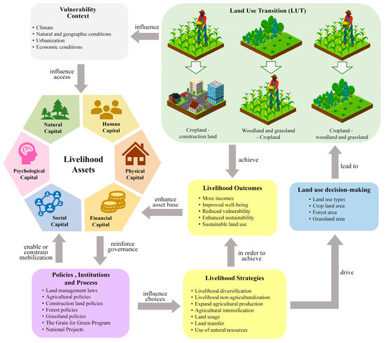
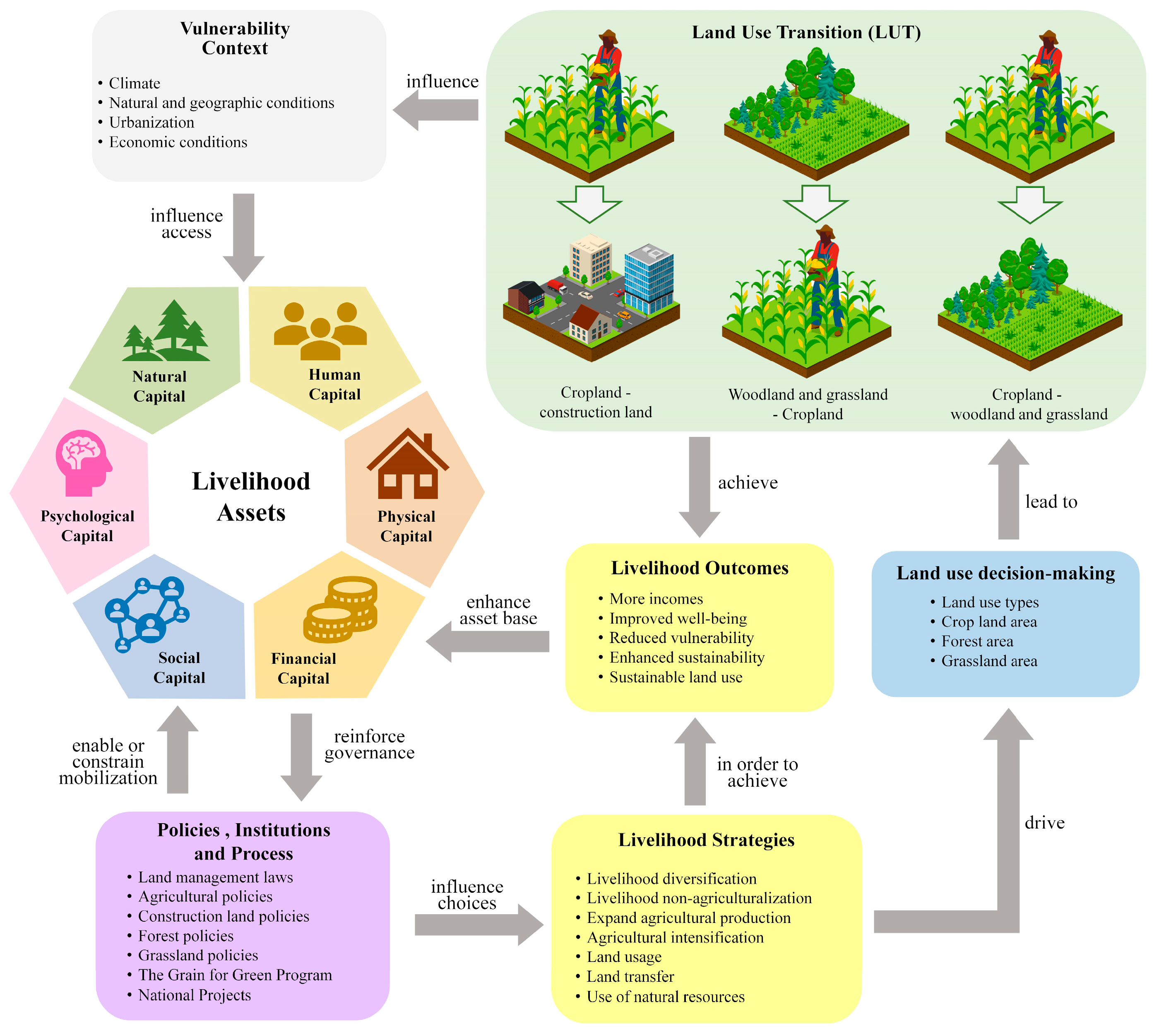
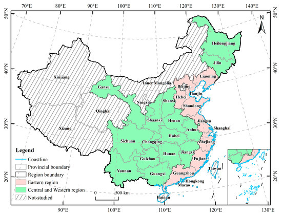
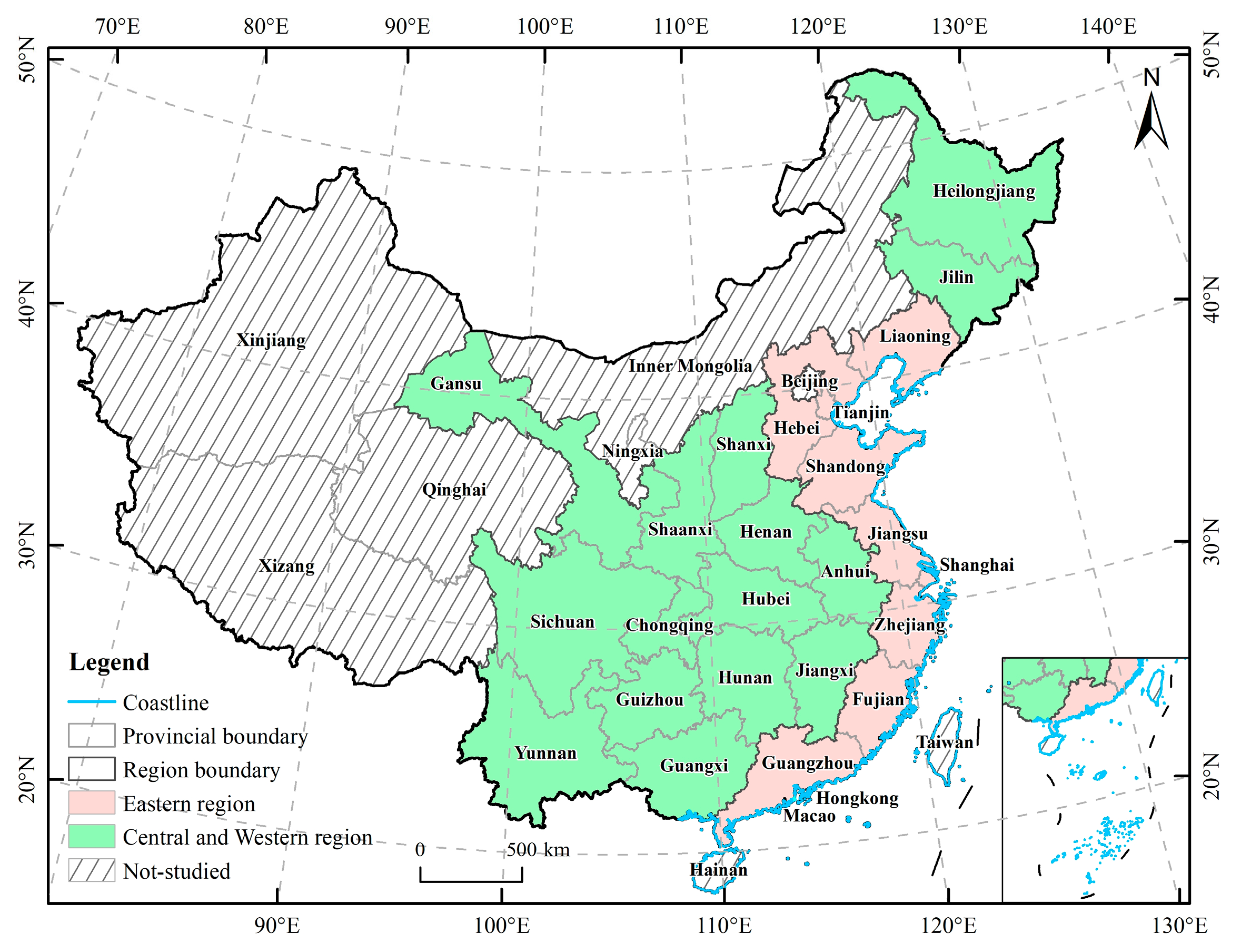
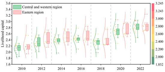
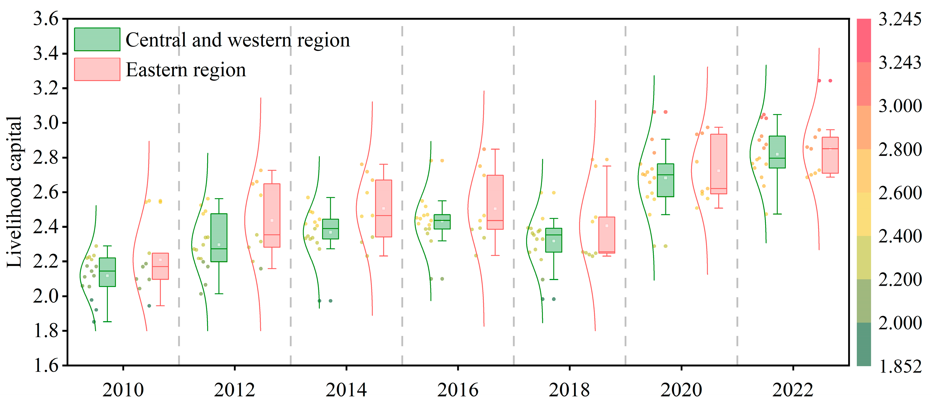
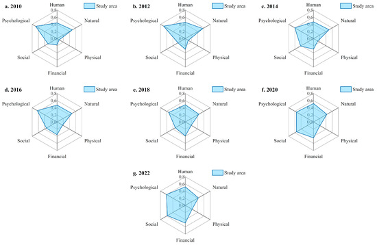
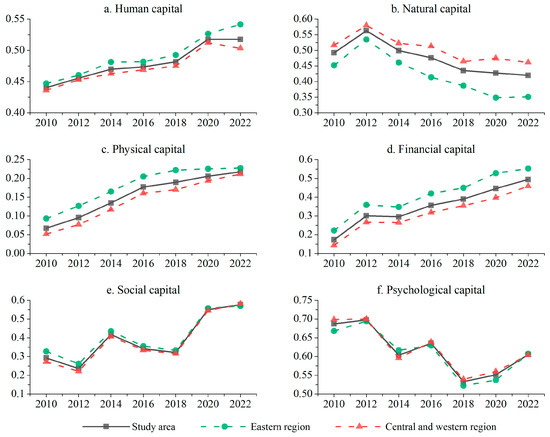
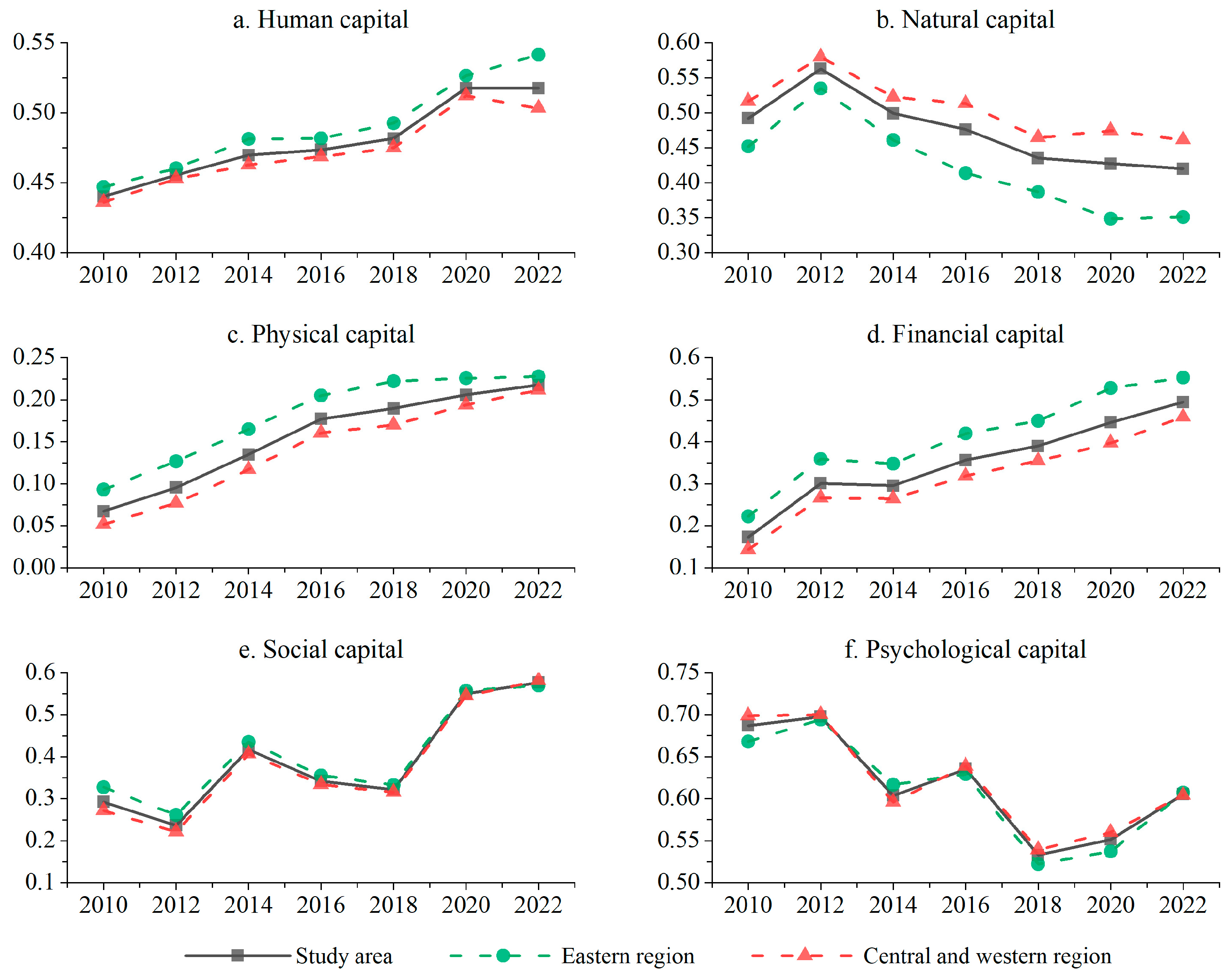
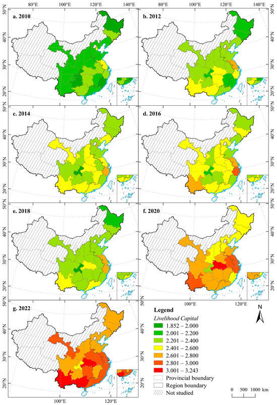
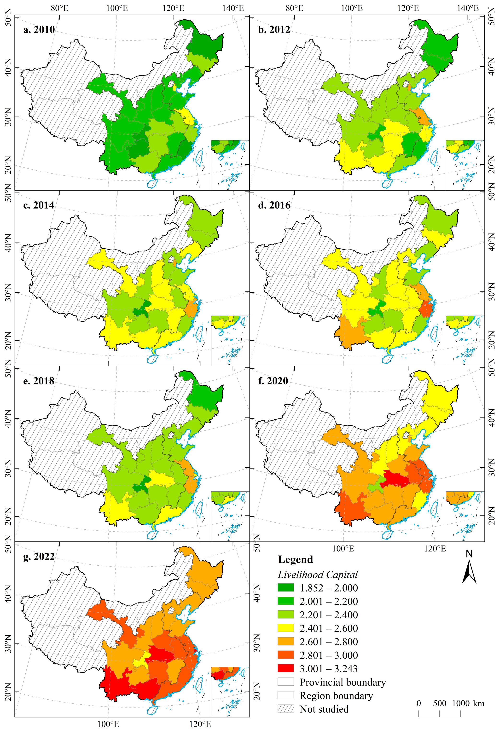
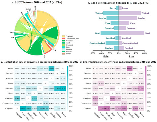
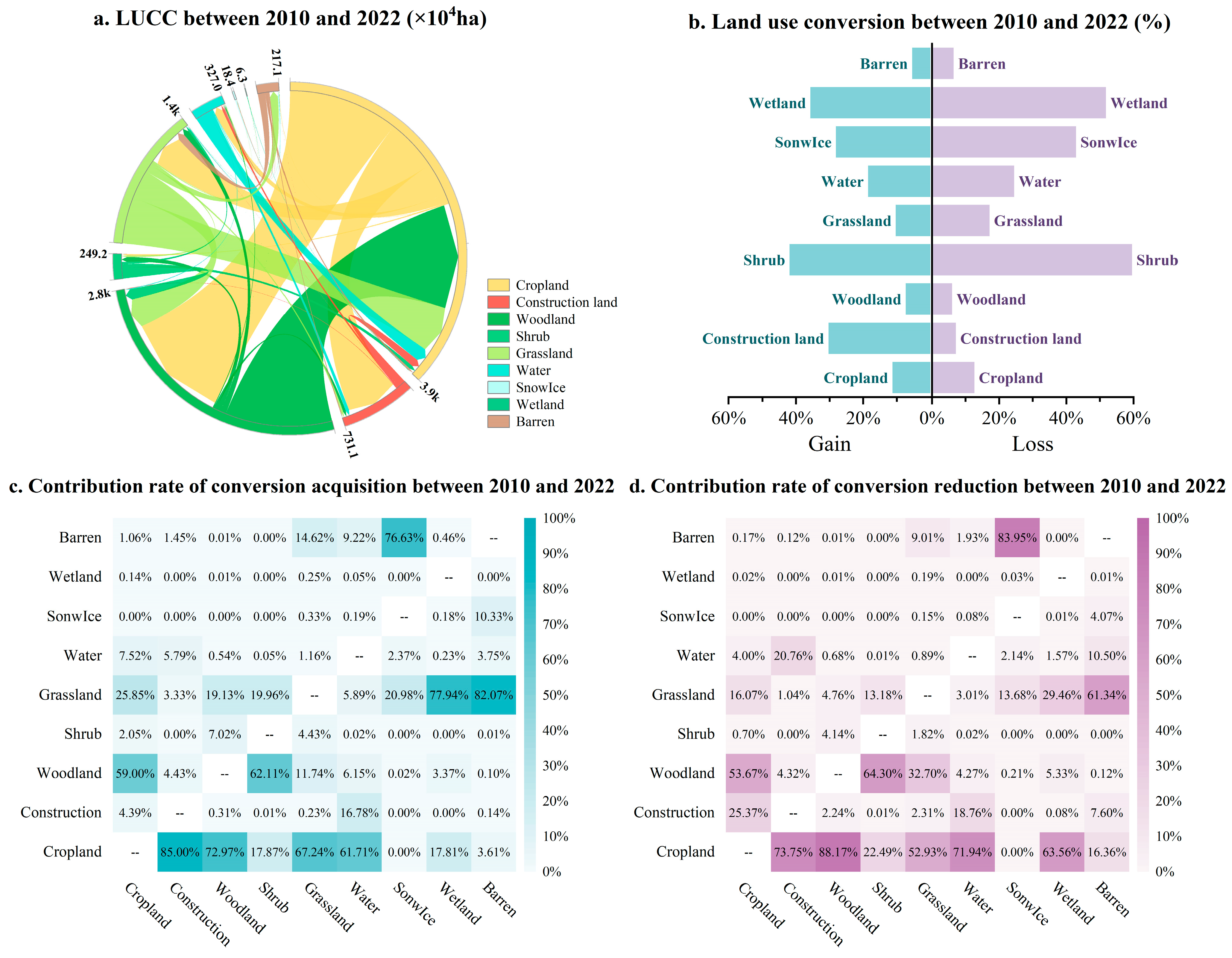
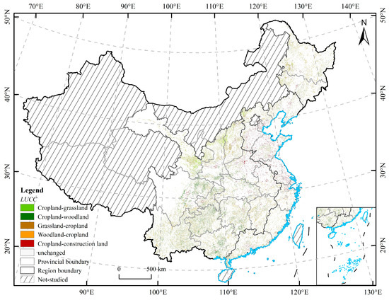
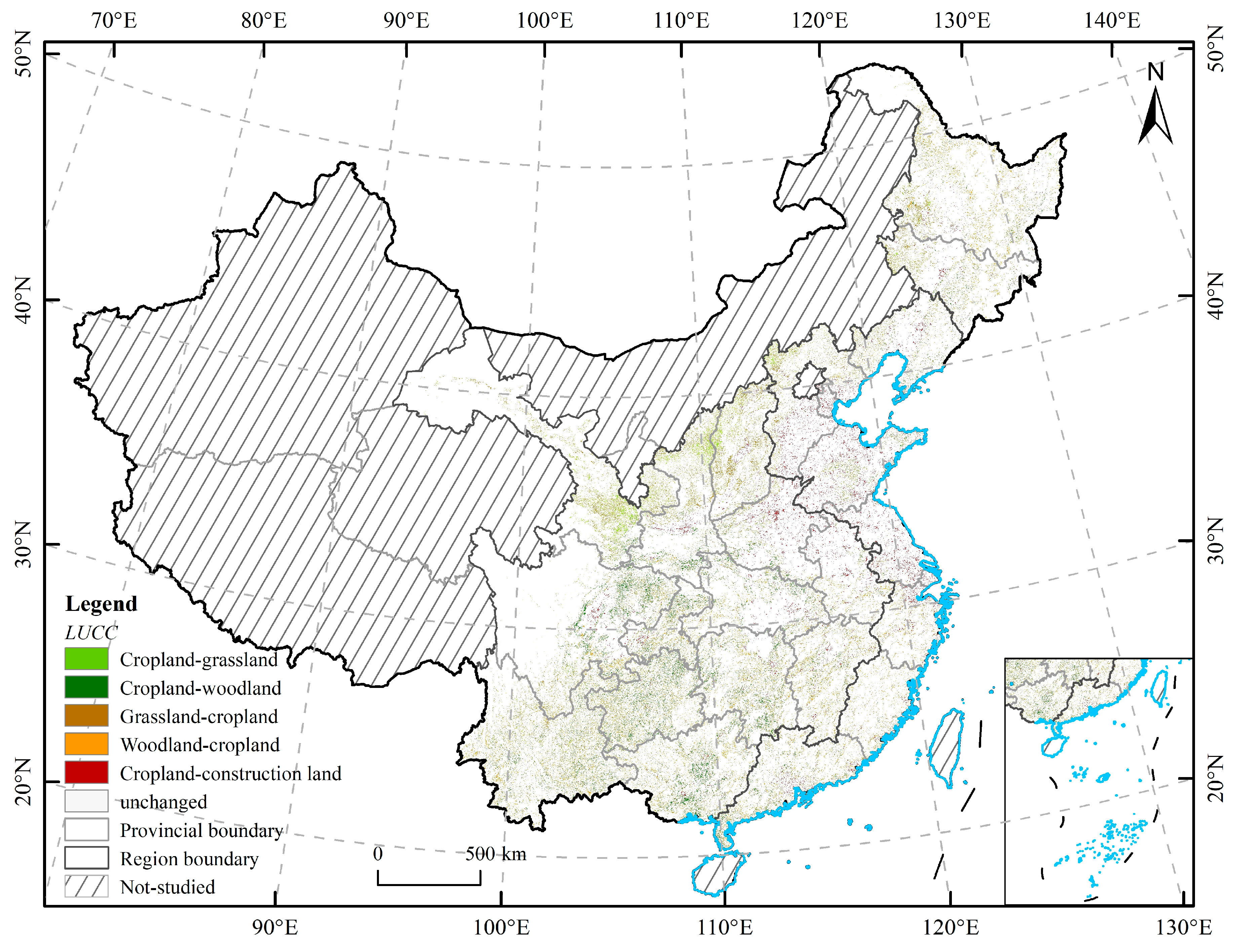
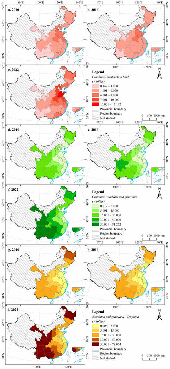
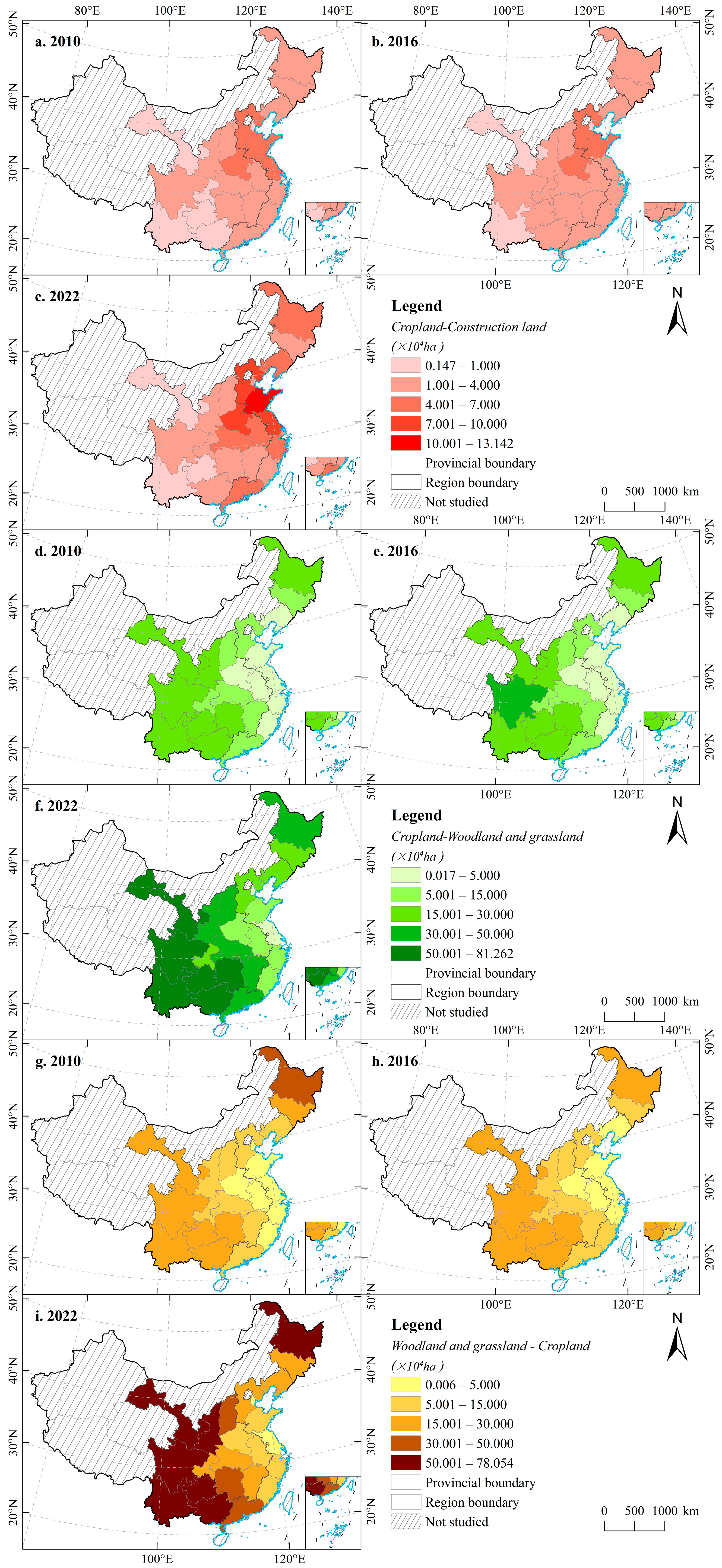

Disclaimer/Publisher’s Note: The statements, opinions and data contained in all publications are solely those of the individual author(s) and contributor(s) and not of MDPI and/or the editor(s). MDPI and/or the editor(s) disclaim responsibility for any injury to people or property resulting from any ideas, methods, instructions or products referred to in the content. |
© 2026 by the authors. Licensee MDPI, Basel, Switzerland. This article is an open access article distributed under the terms and conditions of the Creative Commons Attribution (CC BY) license.